{width=500px}
In the last two lecturs, we discuss a general model for learning, neural networks. ## History and recent surge From [Wang and Raj (2017)](https://arxiv.org/pdf/1702.07800.pdf):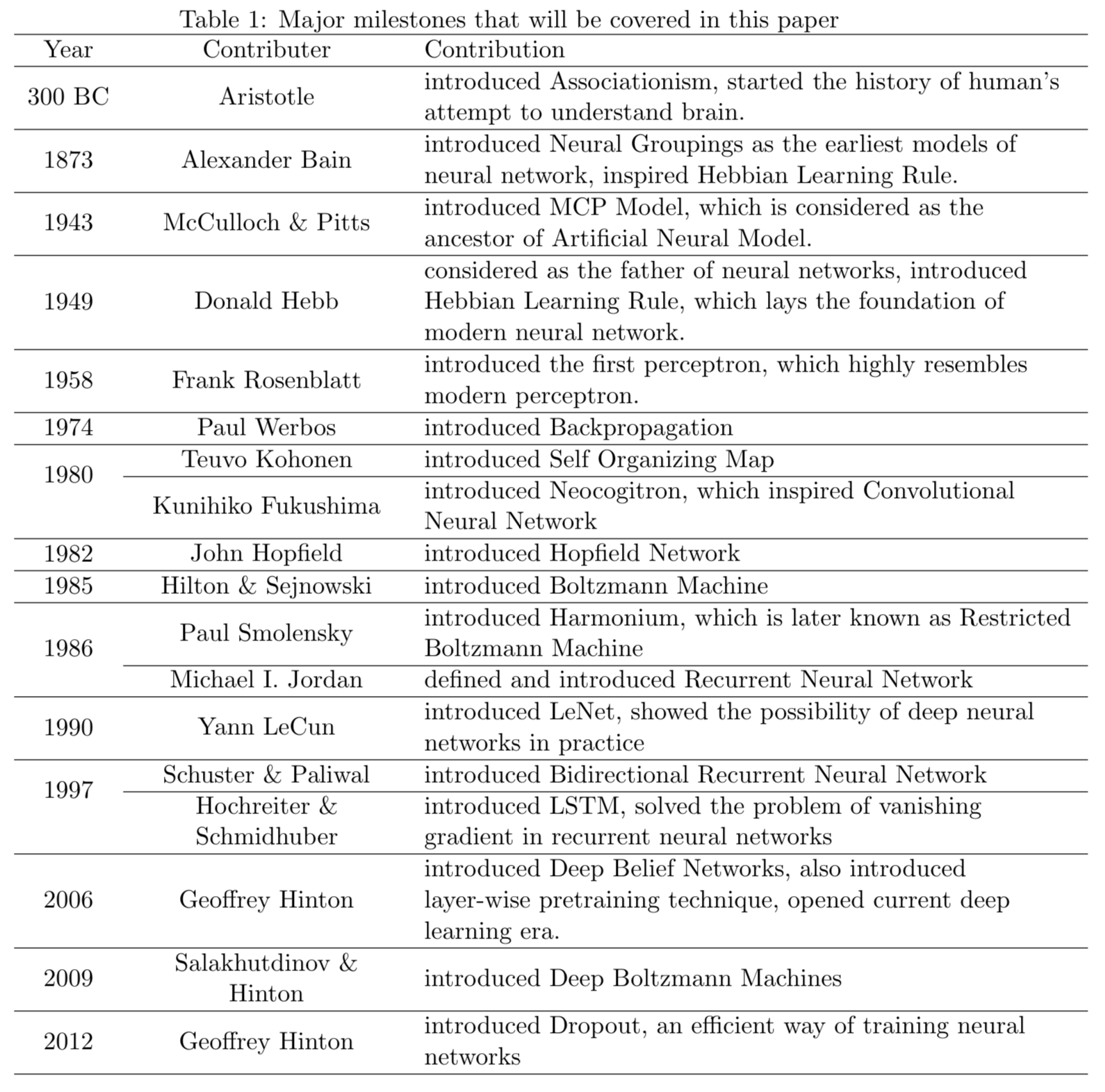{width=500px}
## Learning sources - _Elements of Statistical Learning_ (ESL) Chapter 11: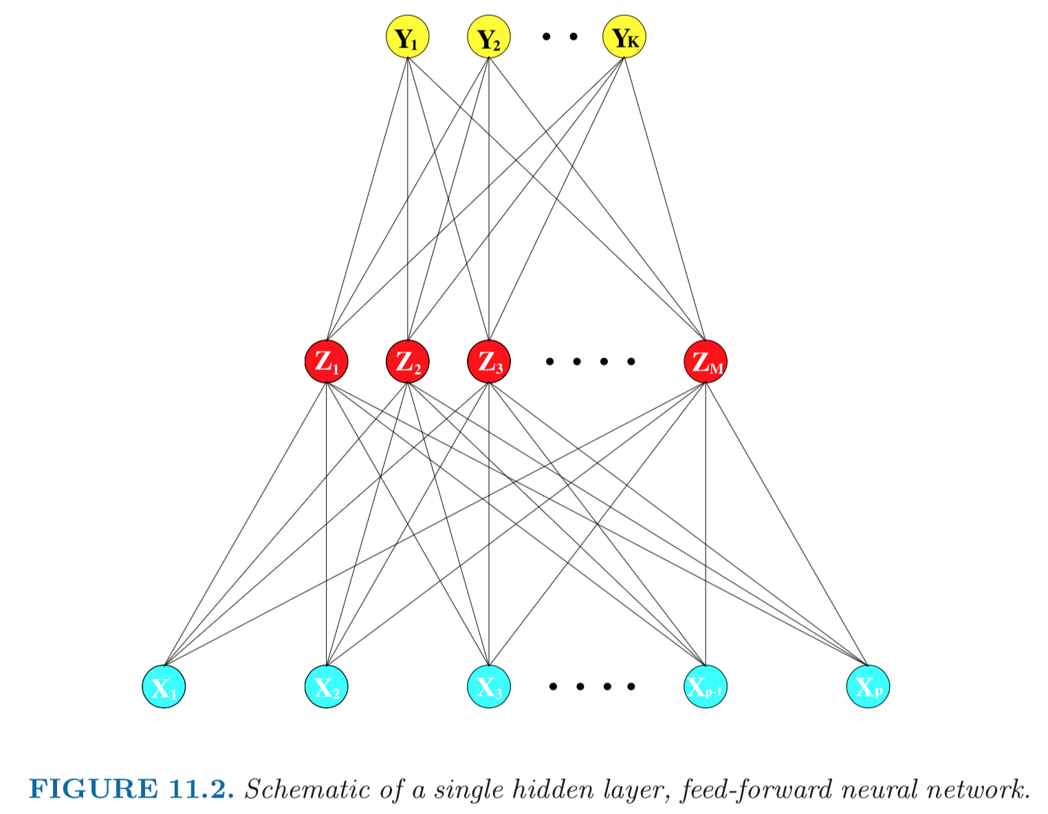{width=500px}
- Mathematical model: \begin{eqnarray*} Z_m &=& \sigma(\alpha_{0m} + \alpha_m^T X), \quad m = 1, \ldots, M \\ T_k &=& \beta_{0k} + \beta_k^T Z, \quad k = 1,\ldots, K \\ Y_k &=& f_k(X) = g_k(T), \quad k = 1, \ldots, K. \end{eqnarray*} - **Output layer**: $Y=(Y_1, \ldots, Y_K)$ are $K$-dimensional output. For univariate response, $K=1$; for $K$-class classification, $k$-th unit models the probability of class $k$. - **Input layer**: $X=(X_1, \ldots, X_p)$ are $p$-dimensional input features. - **Hidden layer**: $Z=(Z_1, \ldots, Z_M)$ are derived features created from linear combinations of inputs $X$. - $T=(T_1, \ldots, T_K)$ are the output features that are directly associated with the outputs $Y$ through output functions $g_k(\cdot)$. - $g_k(T) = T$ for regression. $g_k(T) = e^{T_k} / \sum_{k=1}^K e^{T_k}$ for $K$-class classification (**softmax regression**). - Number of **weights** (parameters) is $M(p+1) + K(M+1)$. - **Activation function** $\sigma$: - $\sigma(v)=$ a step function: human brain models where each unit represents a neuron, and the connections represent synapses; the neurons fired when the total signal passed to that unit exceeded a certain threshold. - **Sigmoid** function: $$ \sigma(v) = \frac{1}{1 + e^{-v}}. $$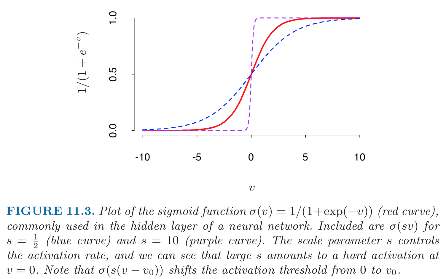{width=500px}
- **Rectifier**. $\sigma(v) = v_+ = max(0, v)$. A unit employing the rectifier is called a **rectified linear unit (ReLU)**. According to Wikipedia: > The rectifier is, as of 2018, the most popular activation function for deep neural networks. - **Softplus**. $\sigma(v) = \log (1 + \exp v)$.{width=400px}
- Given training data $(X_1, Y_1), \ldots, (X_n, Y_n)$, the **loss function** $L$ can be: - Sum of squares error (SSE): $$ L = \sum_{k=1}^K \sum_{i=1}^n [y_{ik} - f_k(x_i)]^2. $$ - Cross-entropy (deviance): $$ L = - \sum_{k=1}^K \sum_{i=1}^n y_{ik} \log f_k(x_i). $$ - Model fitting: **back-propagation** (gradient descent) - Consider sum of squares error and let \begin{eqnarray*} z_{mi} &=& \sigma(\alpha_{0m} + \alpha_m^T x_i) \\ R_i &=& \sum_{k=1}^K [y_{ik} - f_k(x_i)]^2. \end{eqnarray*} - The derivatives: \begin{eqnarray*} \frac{\partial R_i}{\partial \beta_{km}} &=& -2 [y_{ik} - f_k(x_i)] g_k'(\beta_k^T z_i) z_{mi} \equiv \delta_{ki} z_{mi} \\ \frac{\partial R_i}{\partial \alpha_{ml}} &=& - 2 \sum_{k=1}^K [y_{ik} - f_k(x_i)] g_k'(\beta_k^T z_i) \beta_{km} \sigma'(\alpha_m^T x_i) x_{il} \equiv s_{mi} x_{il}. \end{eqnarray*} - Gradient descent update: \begin{eqnarray*} \beta_{km}^{(r+1)} &=& \beta_{km}^{(r)} - \gamma_r \sum_{i=1}^n \frac{\partial R_i}{\partial \beta_{km}} \\ \alpha_{ml}^{(r+1)} &=& \alpha_{ml}^{(r)} - \gamma_r \sum_{i=1}^n \frac{\partial R_i}{\partial \alpha_{ml}}, \end{eqnarray*} where $\gamma_r$ is the **learning rate**. - Back-propagation equations $$ s_{mi} = \sigma'(\alpha_m^T x_i) \sum_{k=1}^K \beta_{km} \delta_{ki}. $$ - Two-pass updates: \begin{eqnarray*} & & \text{initialization} \to \hat f_k(x_i) \quad \quad \quad \text{(forward pass)} \\ &\to& \delta_{ki} \to s_{mi} \to \hat \beta_{km} \text{ and } \hat \alpha_{ml} \quad \quad \text{(backward pass)}. \end{eqnarray*} - Advantages: each hidden units passes and receives information only to and from units that share a connection; can be implemented efficiently on a parallel architecture computer. - Stochastic gradient descent (**SGD**). In real machine learning applications, training set can be large. Back-propagation over all training cases can be expensive. Learning can also be carried out **online** — processing each batch one at a time, updating the gradient after each training batch, and cycling through the training cases many times. A training **epoch** refers to one sweep through the entire training set. **AdaGrad** and **RMSProp** improve the stability of SGD by trying to incorpoate Hessian information in a computationally cheap way. - The **unversal approximation theorem** states that a feed-forward network with a single hidden layer containing a finite number of neurons can approximate continuous functions on compact subsets of $\mathbb{R}^n$, under mild assumptions on the activation function. - Neural network model is a **projection pursuit** type additive model: $$ f(X) = \beta_0 + \sum_{m=1}^M \beta_m \sigma(\alpha_{m0} + \alpha_M^T X). $$ ## Multi-layer neural network - Aka multi-layer perceptron (MLP). - 1 hidden layer: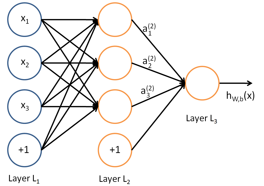{width=400px}
- 2 hidden layers: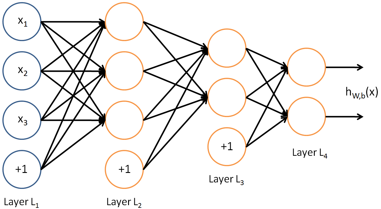{width=400px}
## Practical issues Neural networks are **not a fully automatic tool**, as they are sometimes advertised; as with all statistical models, subject matter knowledge should and often be used to improve their performance. - Starting values: usually starting values for weights are chosen to be random values near zero; hence the model starts out nearly linear (for sigmoid), and becomes nonlinear as the weights increase. - Overfitting (too many parameters): 1. early stopping; 2. weight decay by $L_2$ penalty $$ L(\alpha, \beta) + \frac{\lambda}{2} \left( \sum_{k, m} \beta_{km}^2 + \sum_{m, l} \alpha_{ml}^2 \right). $$ $\lambda$ is the **weight decay parameter**. 3. **Dropout**. At each training case, individual nodes are either dropped out of the net with probability $1-p$ or kept with probability $p$, so that a reduced network is left; incoming and outgoing edges to a dropped-out node are also removed. Forward and backpropagation for that training case are done only on this thinned network.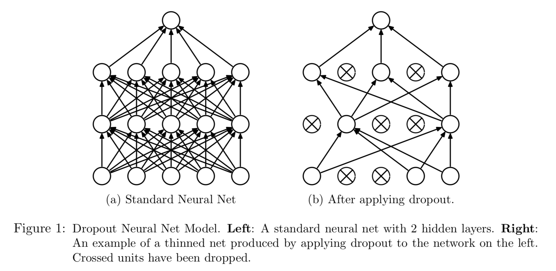{width=500px}
Figure from [Srivastava, Hinton, Krizhevsky, Sutskever, and Salakhutdinov (2014)](https://www.cs.toronto.edu/~hinton/absps/JMLRdropout.pdf). - Scaling of inputs: mean 0 and standard deviation 1. With standardized inputs, it is typical to take random uniform weights over the range [−0.7,+0.7]. - How many hidden units and how many hidden layers: guided by domain knowledge and experimentation. - Multiple minima: try with different starting values. ## Convolutional neural networks (CNN) Sources: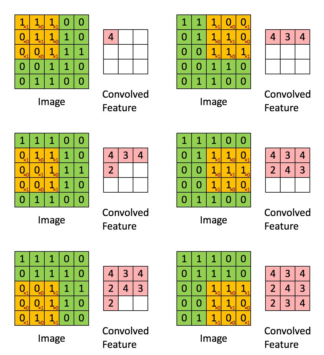{width=400px}
Consider $96 \times 96$ images. For each feature, first learn a $8 \times 8$ **feature detector** (or **filter** or **kernel**) from (possibly randomly sampled) $8 \times 8$ patches from the larger image. Then apply the learned detector to all $8 \times 8$ regions of the $96 \times 96$ image to obtain one $89 \times 89$ convolved feature for that feature. From [Wang and Raj (2017)](https://arxiv.org/pdf/1702.07800.pdf):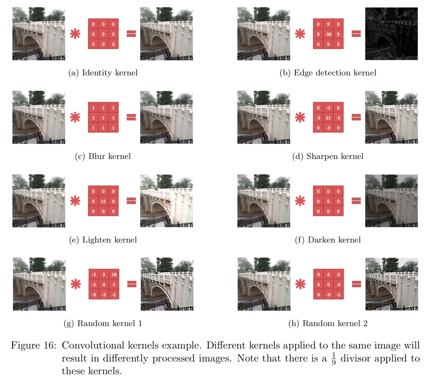{width=700px}
- **Pooling**. For a neural network with 100 hidden units, we have $89^2 \times 100 = 792,100$ convolved features. This can be reduced by calculating the mean (or max) vale of a particular feature over a region of the image. These summary statistics are much lower in dimension (compared to using all of the extracted features) and can also improve results (less over-fitting). We call this aggregation operation **pooling**, or sometimes **mean pooling** or **max pooling** (depending on the pooling operation applied).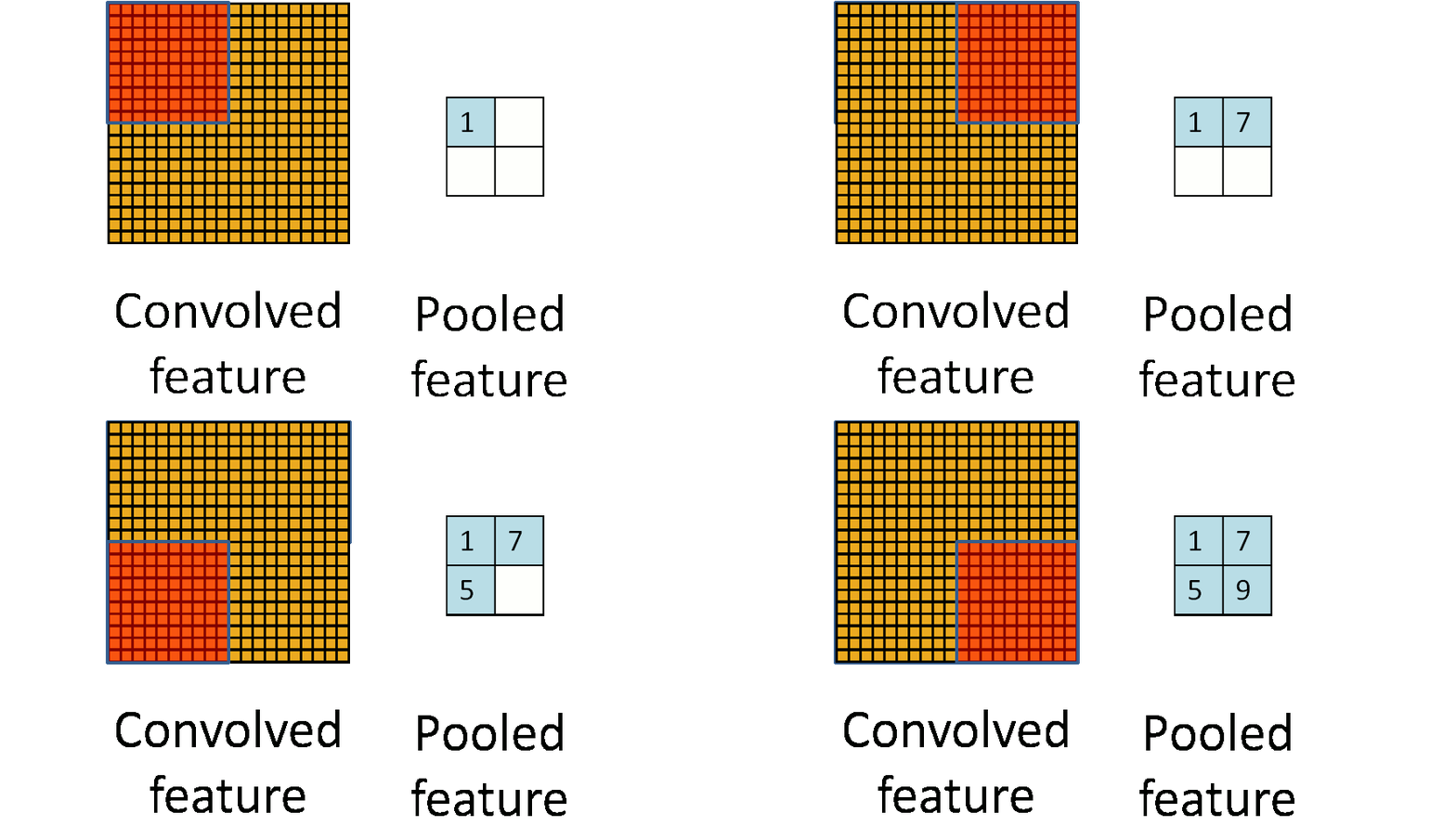{width=400px}
- **Convolutional neural network (CNN)**. Convolution + pooling + multi-layer neural networks.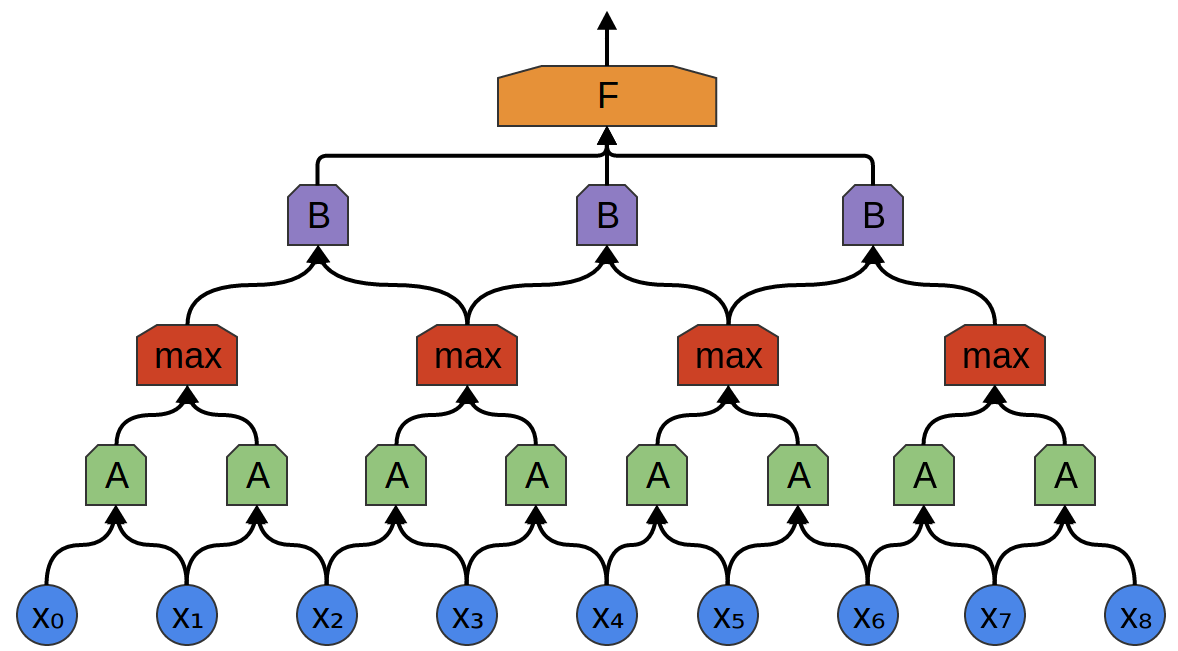{width=500px} 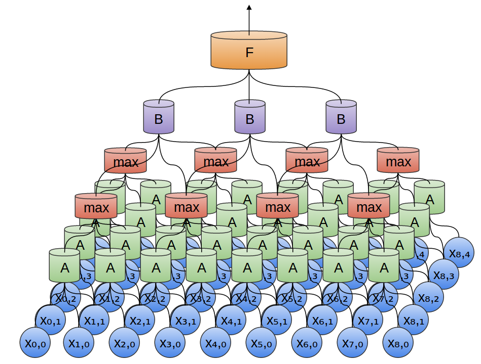{width=500px}
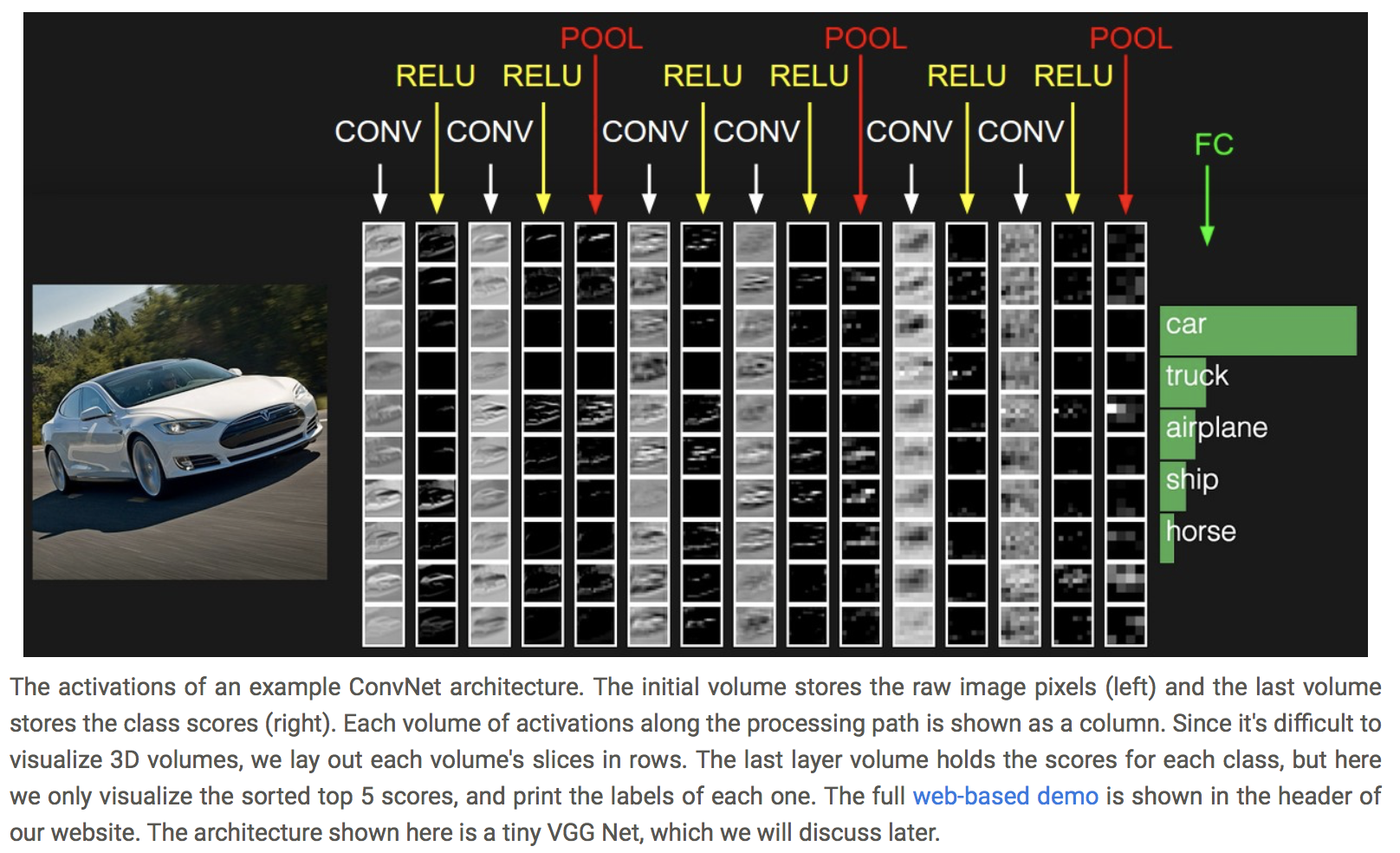{width=700px}
## Example: handwritten digit recognition.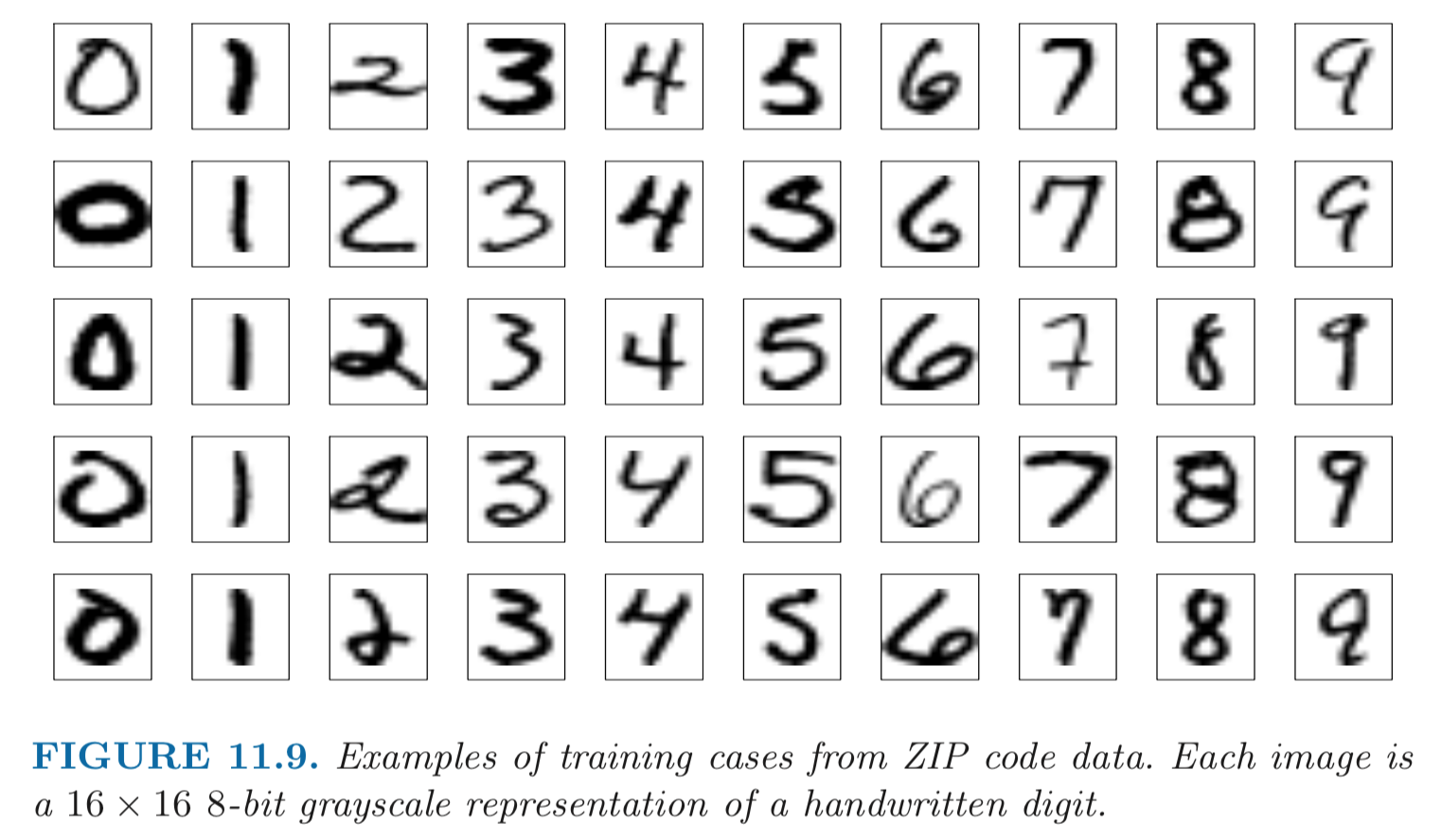{width=500px}
- Input: 256 pixel values from $16 \times 16$ grayscale images. Output: 0, 1, ..., 9 10 class-classification. - A modest experiment subset: 320 training digits and 160 testing digits. - net-1: no hidden layer, equivalent to multinomial logistic regression. net-2: one hidden layer, 12 hidden units fully connected. net-3: two hidden layers locally connected. net-4: two hidden layers, locally connected with weight sharing. net-5: two hidden layers, locally connected, two levels of weight sharing (was the result of many person years of experimentation).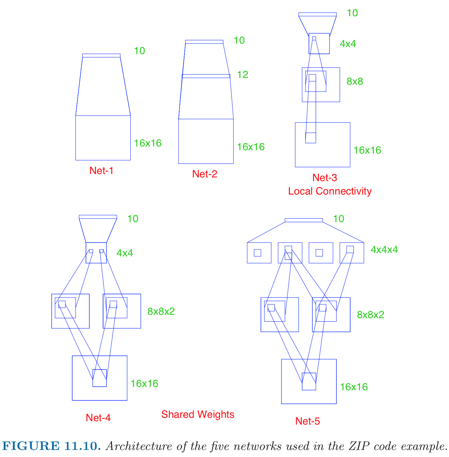{width=500px}
- Results: | network | links | weights | accuracy | |---------|-------|---------|----------| | net 1 | 2570 | 2570 | 80.0% | | net 2 | 3124 | 3214 | 87.0% | | net 3 | 1226 | 1226 | 88.5% | | net 4 | 2266 | 1131 | 94.0% | | net 5 | 5194 | 1060 | 98.4% | Net-5 and similar networks were start-of-the-art in early 1990s. - On the larger benchmark dataset **MNIST** (60,000 training images, 10,000 testing images), accuracies of following methods were reported: | Method | Error rate | |--------|----------| | tangent distance with 1-nearest neighbor classifier | 1.1% | | degree-9 polynomial SVM | 0.8% | | LeNet-5 | 0.8% | | boosted LeNet-4 | 0.7% | ## Example: image classification - [Krizhevsky, Sutskever, Hinton (2012)](http://www.cs.toronto.edu/~fritz/absps/imagenet.pdf) - [ImageNet](http://www.image-net.org) dataset. Classify 1.2 million high-resoultion images into 1000 classes. - A combination of techniques: GPU, ReLU, DropOut. - 5 convolutional layers, pooling interspersed, 3 fully connected layers. 60 million parameters, 650,000 neurons.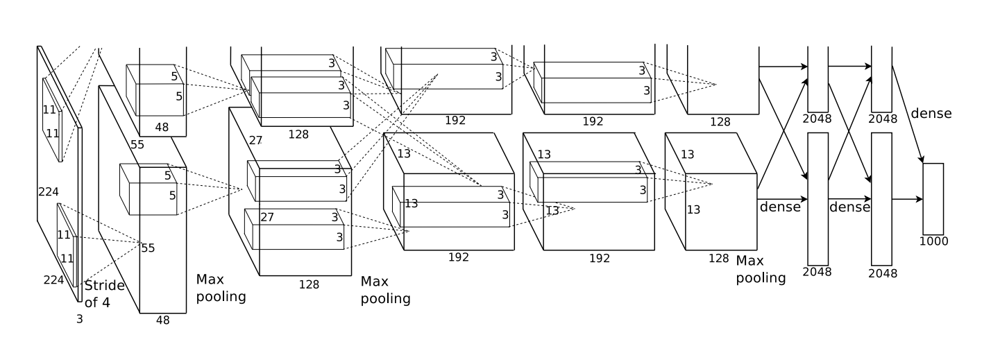{width=500px}
- Achieved 63% accuracy: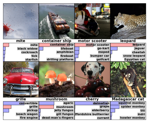{width=500px}
96 learnt filters: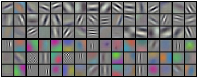{width=500px}
## Recurrent neural networks (RNN) Souces:{width=500px}
- RNNs allow us to operate over sequences of vectors: sequences in the input, the output, or in the most general case both. - Applications of RNN: - [Language modeling and generating text](http://karpathy.github.io/2015/05/21/rnn-effectiveness/). E.g., search prompt, messaging prompt, ...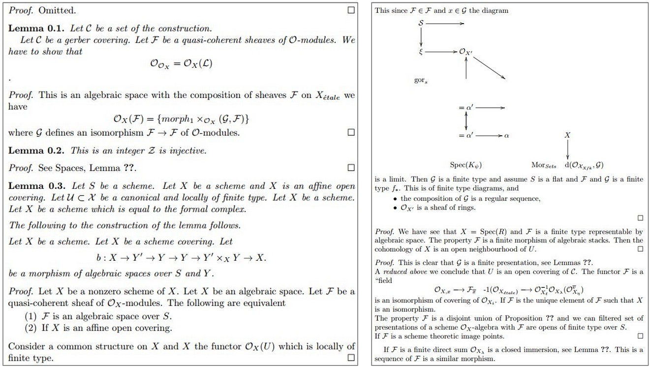{width=500px}
Above: generated (fake) LaTeX on algebraic geometry; see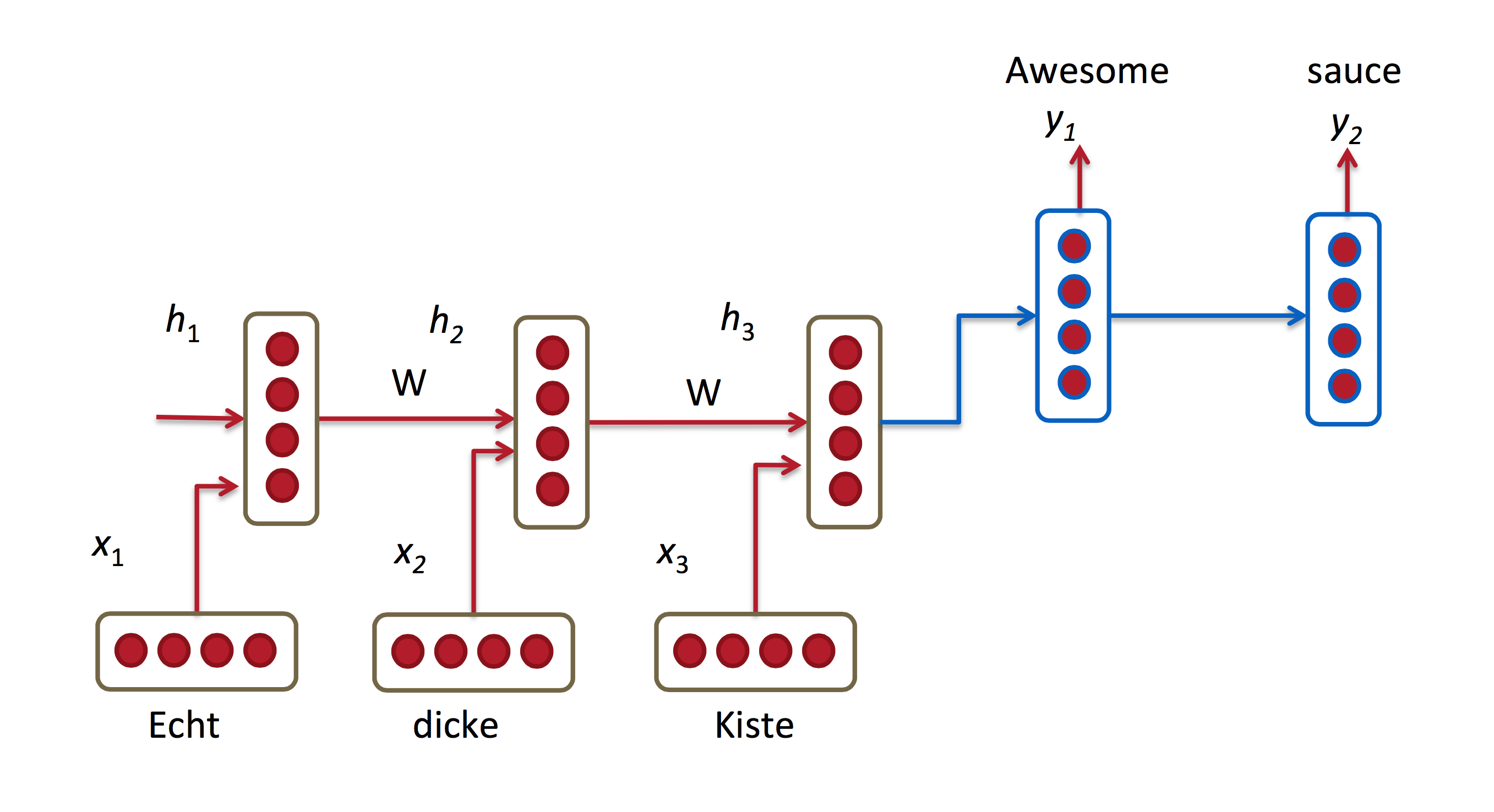{width=500px}
- **Computer vision**: image captioning, video captioning, ...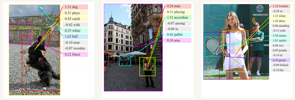{width=500px}
- RNNs accept an input vector $x$ and give you an output vector $y$. However, crucially this output vector’s contents are influenced not only by the input you just fed in, but also on the entire history of inputs you’ve fed in the past. - Short-term dependencies: to predict the last word in "the clouds are in the _sky_":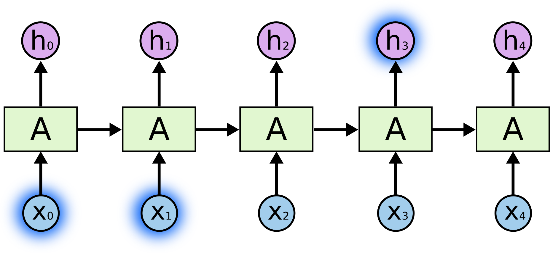{width=500px}
- Long-term dependencies: to predict the last word in "I grew up in France... I speek fluent _French_":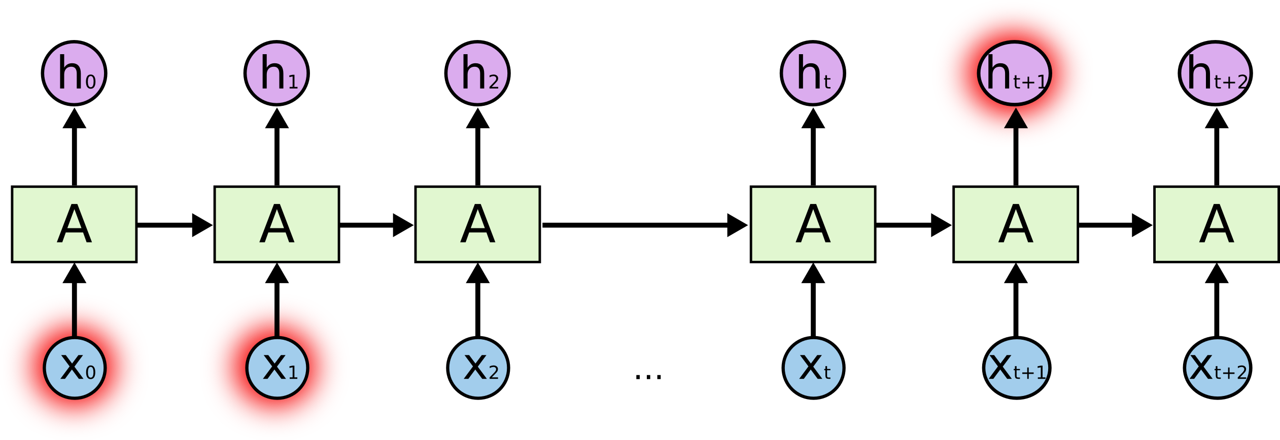{width=500px}
- Typical RNNs are having trouble with learning long-term dependencies.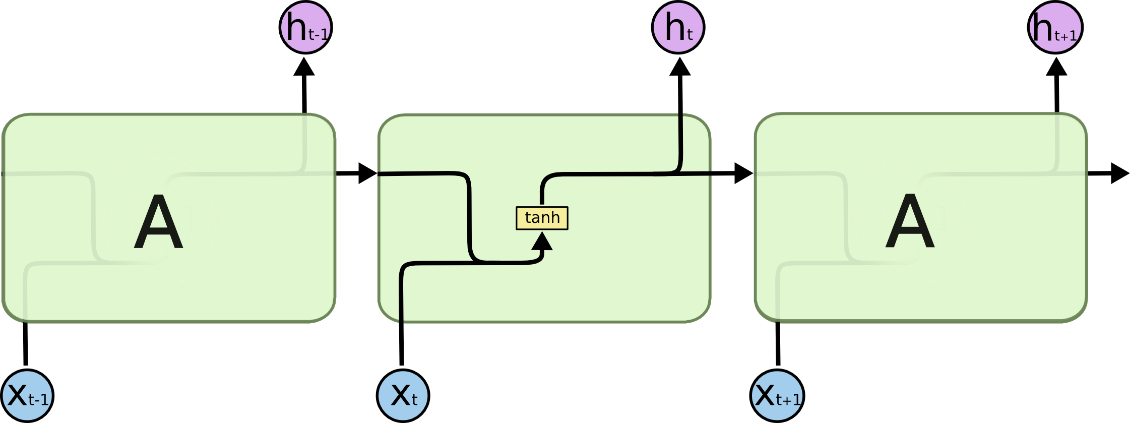{width=500px}
- **Long Short-Term Memory networks (LSTM)** are a special kind of RNN capable of learning long-term dependencies.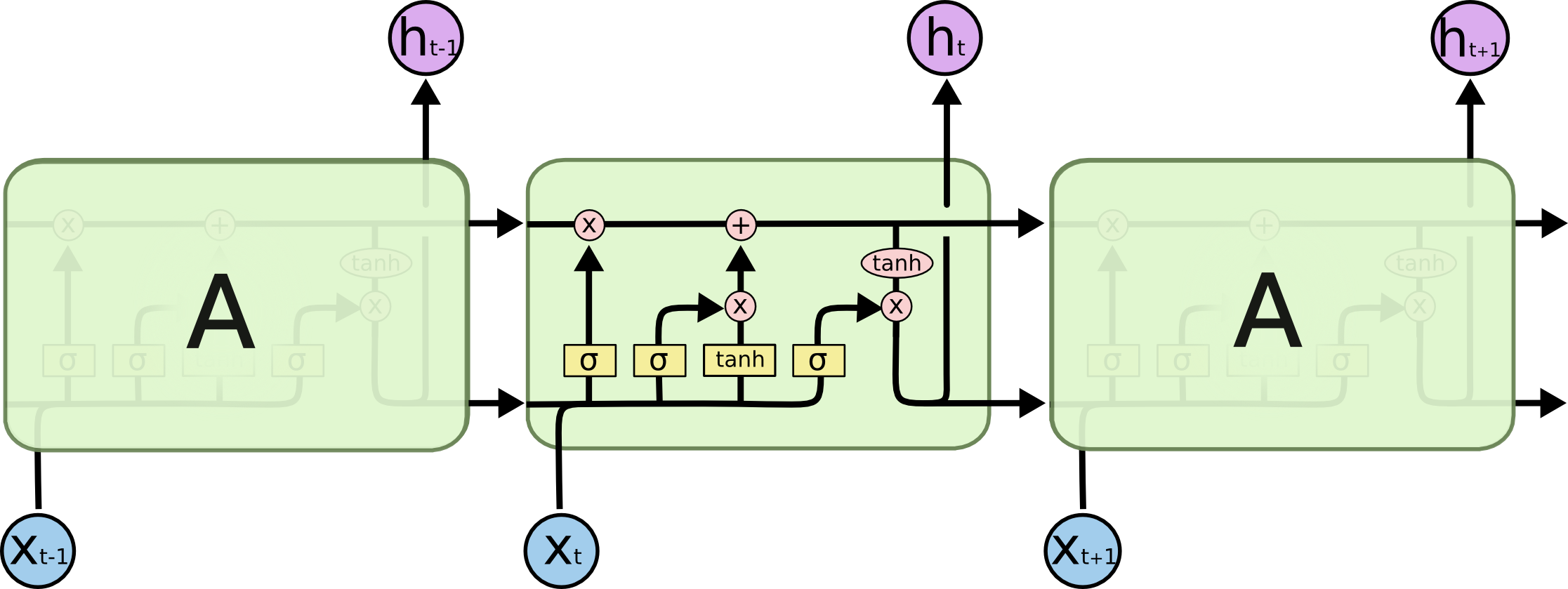{width=500px} {width=500px}
The **cell state** allows information to flow along it unchanged.{width=500px}
The **gates** give the ability to remove or add information to the cell state.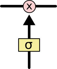{width=100px}