---
title: "Select Topics in R Programming - Part II"
author: "Dr. Hua Zhou @ UCLA"
date: "Jan 22, 2019"
subtitle: Biostat M280
output:
html_document:
toc: true
toc_depth: 4
---
```{r setup, include=FALSE}
knitr::opts_chunk$set(echo = TRUE)
options(width = 120)
```
```{r}
sessionInfo()
```
## Typical development cycle for computational statistics
1. Scientific planning: What experiments would verify/invalidate our hypotheses? What parameter settings should we consider?
0. Code planning: What does the code need to do? How will the code fit together? What functions will be used? What are their inputs/outputs etc.
0. Implementation:
1. Prototype functions, classes, etc., partial documentation
2. Write unit tests
3. Implement code, run unit tests, debug
4. Broader testing, more debugging
5. Profile code, identify bottlenecks
6. Optimize code
0. Conduct experiments.
0. Full documentation.
## Bytecode compilation
- After profiling, what to do to improve performance?
1. Ask are there obvious speedups? Are things being computed unnecessarily? Are you using a `data.frame` where you should be using a matrix etc.
2. Look up your problem (e.g., search for "lapply slow" or "speeding up `lapply`" etc.)
3. Try the just-in-time (JIT) compiler.
4. Consider re-writing some or all of the code in a compiled language (e.g., C/C++).
5. Try parallelization.
- R typical execution:
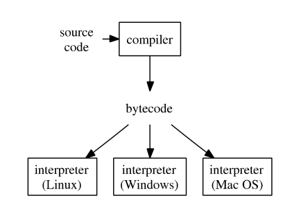{width=400px}
- [Julia illustration](http://hua-zhou.github.io/teaching/biostatm280-2017spring/slides/02-juliaintro/juliaintro.html#Just-in-time-compilation-(JIT)).
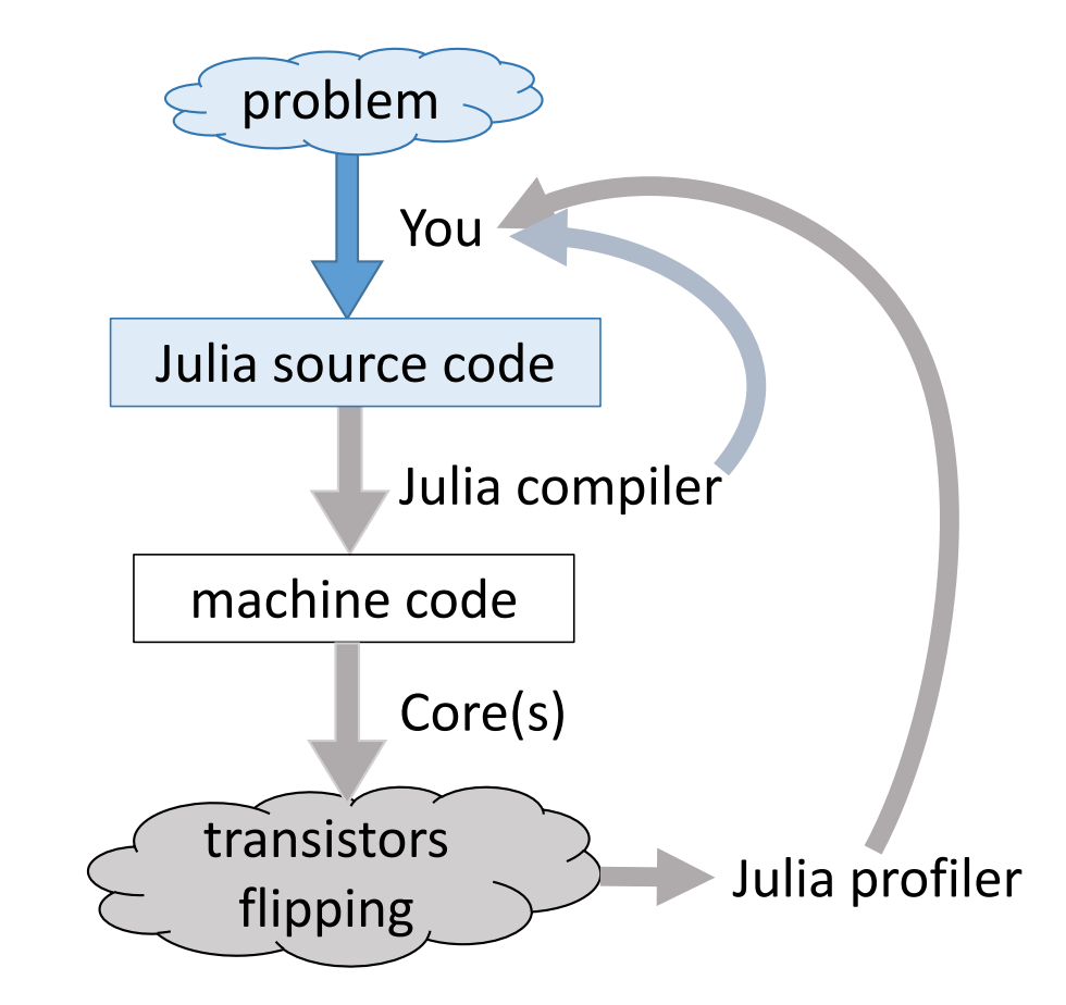{width=400px} 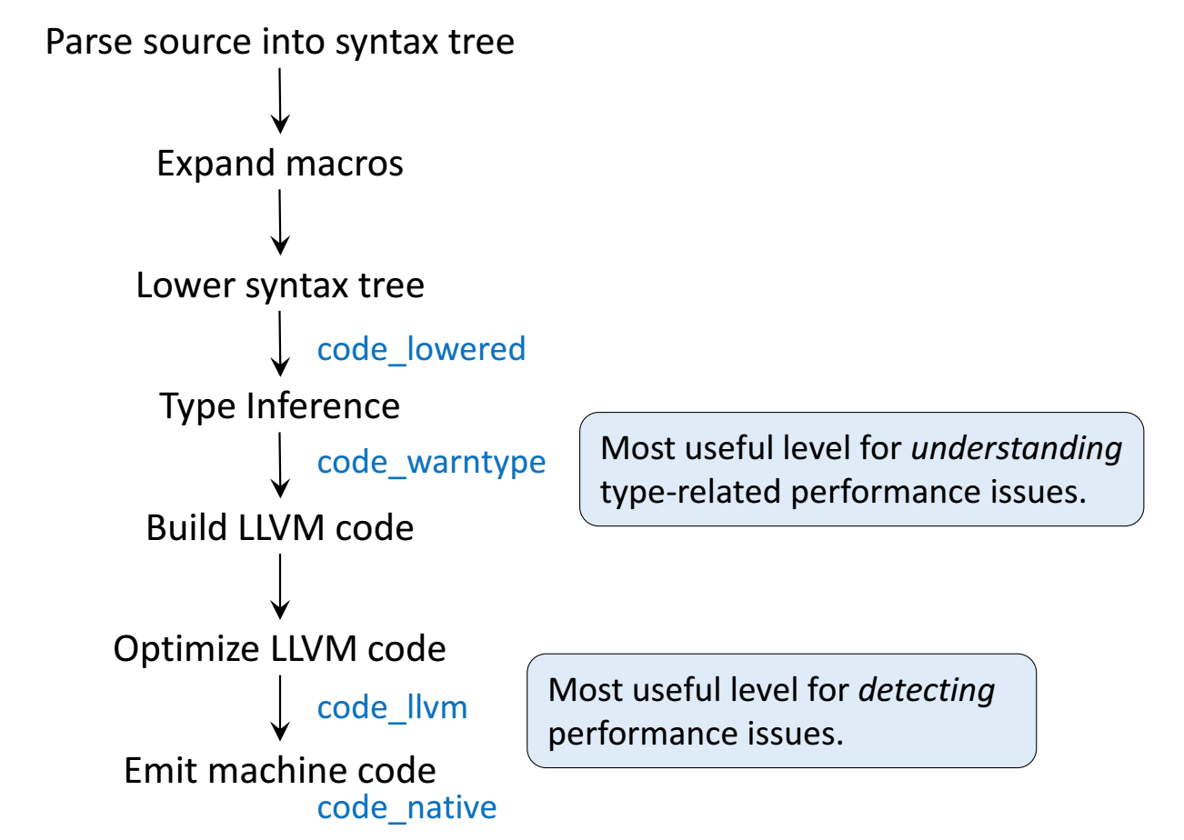{width=400px}
- Since R 2.1.4, the `compiler` package by Luke Tierney is distributed with base R. `compiler` package compiles an R function into bytecode.
### Example: summing a vector
Brute-force `for` loop for summing a vector:
```{r}
sum_r <- function(x) {
sumx <- 0.0
for (i in 1:length(x)) {
sumx <- sumx + x[i]
}
return(sumx)
}
sum_r
```
Run the code on 1e6 elements:
```{r}
library(microbenchmark)
library(ggplot2)
x = seq(from = 0, to = 100, by = 0.0001)
microbenchmark(sum_r(x))
```
Let's compile the function into bytecode `sum_rc` and benchmark again:
```{r}
library(compiler)
sum_rc <- cmpfun(sum_r)
sum_rc
```
Benchmark again:
```{r}
microbenchmark(sum_r(x), sum_rc(x))
```
**Surprise**! **Surprise**! Compiling into bytecode does not help at all. Following code shows that the function `sum_r` is already compiled into bytecode before execution.
```{r}
sum_r
```
Let's turn off JIT (just-in-time compilation), re-define the (same) `sum_r` function, and benchmark again:
```{r}
enableJIT(0) # set JIT leval to 0
sum_r <- function(x) {
sumx <- 0.0
for (i in 1:length(x)) {
sumx <- sumx + x[i]
}
return(sumx)
}
microbenchmark(sum_r(x))
```
Now we witness the slowness of the un-compiled `sum_r`.
Documentation of `enableJIT`:
> enableJIT enables or disables just-in-time (JIT) compilation. JIT is disabled if the argument is 0. If level is 1 then larger closures are compiled before their first use. If level is 2, then some small closures are also compiled before their second use. If level is 3 then in addition all top level loops are compiled before they are executed. JIT level 3 requires the compiler option optimize to be 2 or 3. The JIT level can also be selected by starting R with the environment variable R_ENABLE_JIT set to one of these values. Calling enableJIT with a negative argument returns the current JIT level. The default JIT level is 3.
Since R 3.4.0 (Apr 2017), the JIT (‘Just In Time’) bytecode compiler is enabled by default at its level 3.
If you create a package, then you automatically compile the package on installation by adding
```{r, eval = FALSE}
ByteCompile: true
```
to the `DESCRIPTION` file.
Note Matlab has employed JIT technology since **2002** and Julia is designed totally based on JIT. R finally is on the same boat.
## Rcpp
Learning sources:
- _Advanced R_:
`compiler` package compiles R code into bytecode, which is translated to machine code by interpreter during execution. A low-level language such as C, C++, and Fortran is compiled into machine code directly, yielding the maximum efficiency.
### Use `cppFunction`
`Rcpp` package provides a convenient way to embed C++ code in R code.
```{r}
library(Rcpp)
cppFunction('double sum_c(NumericVector x) {
int n = x.size();
double total = 0;
for(int i = 0; i < n; ++i) {
total += x[i];
}
return total;
}')
sum_c
```
Benchmark (1) compiled C++ function `sum_c` together with (2) R function `sum_r`, (3) compiled R function `sum_rc`, and (4) the `sum` function in base R:
```{r}
mbm <- microbenchmark(sum_r(x), sum_rc(x), sum_c(x), sum(x))
mbm
autoplot(mbm)
```
**Remember we turned off JIT by `enableGIT(0)` earlier.**
### Use `sourceCpp`
In realistic projects, we write standalone C++ files and then source them into R using `sourceCpp()`. For example
```{bash}
cat sum.cpp
```
```{r}
sourceCpp("sum.cpp")
sum_c
```
### [Julia](https://julialang.org)
As a Julia fan, I want to see how Julia works on this example. `sum_j` is Julia equivalent of the `sum_r` function:
```{julia}
# Julia code in this chunk
using BenchmarkTools
function sum_j(x)
total = zero(eltype(x))
for xi in x
total += xi
end
total
end
sum_j(1:10)
x = collect(0:0.0001:100);
@benchmark sum_j(x) samples=100
```
Julia retains the claritiy of a high-level language, while achieving efficiency of a low-level language!
My suggestion: avoid all these hassles of **two language problem**, just use Julia 😄
## Parallel computing
- Fact: base R is single-threaded. Even you request a fancy instance with 96 vCPUs, running R code is just using 1/96th of its power.
- To perform multi-core computation in R:
1. Option 1: Manually run multiple R sessions.
2. Option 2: Make multiple `system("Rscript")` calls. Typically automated
by a scripting language (Python, Perl, shell script) or within R (HW1 Q3.
3. Option 3: Use package `parallel`.
- `parallel` package in R.
- Authors: Brian Ripley, Luke Tieney, Simon Urbanek.
- Included in base R since 2.14.0 (2011).
- Based on the `snow` (Luke Tierney) and `multicore` (Simon Urbanek) packages.
- To find the number of cores:
```{r}
library(parallel)
detectCores()
```
### Simulation example
Let's re-visit the simulation example considered in earlier lecture and [HW1 Q4](http://hua-zhou.github.io/teaching/biostatm280-2019winter/hw/hw1/hw1.html).
We have a "new" method that estimates the population mean by averaging the observations indexed by prime numbers.
```{r}
## check if a given integer is prime
isPrime = function(n) {
if (n <= 3) {
return (TRUE)
}
if (any((n %% 2:floor(sqrt(n))) == 0)) {
return (FALSE)
}
return (TRUE)
}
## estimate mean only using observation with prime indices
estMeanPrimes = function(x) {
n <- length(x)
ind <- sapply(1:n, isPrime)
return (mean(x[ind]))
}
```
We want to compare our method to the traditional sample average estimator by simulation studies.
```{r}
## compare methods: sample avg and prime-indexed avg
compare_methods <- function(dist = "gaussian", n = 100, reps = 100, seed = 123) {
# set seed according to command argument `seed`
set.seed(seed)
# preallocate space to store estimators
msePrimeAvg <- 0.0
mseSamplAvg <- 0.0
# loop over simulation replicates
for (r in 1:reps) {
# simulate data according to command arguments `n` and `distr`
if (dist == "gaussian") {
x = rnorm(n)
} else if (dist == "t1") {
x = rcauchy(n)
} else if (dist == "t5") {
x = rt(n, 5)
} else {
stop(paste("unrecognized dist: ", dist))
}
# prime indexed mean estimator and classical sample average estimator
msePrimeAvg <- msePrimeAvg + estMeanPrimes(x)^2
mseSamplAvg <- mseSamplAvg + mean(x)^2
}
mseSamplAvg <- mseSamplAvg / reps
msePrimeAvg <- msePrimeAvg / reps
return(c(mseSamplAvg, msePrimeAvg))
}
```
### Serial code
We need to loop over 3 generative models (`distTypes`) and 20 samples sizes (`nVals`). That are 60 embarssingly parallel tasks.
```{r}
seed = 280
reps = 500
nVals = seq(100, 1000, by = 50)
distTypes = c("gaussian", "t5", "t1")
```
This is the serial code that double-loop over combinations of `distTypes` and `nVals`:
```{r}
## simulation study with combination of generative model `dist` and
## sample size `n` (serial code)
simres1 = matrix(0.0, nrow = 2 * length(nVals), ncol = length(distTypes))
i = 1 # entry index
system.time(
for (dist in distTypes) {
for (n in nVals) {
#print(paste("n=", n, " dist=", dist, " seed=", seed, " reps=", reps, sep=""))
simres1[i:(i + 1)] = compare_methods(dist, n, reps, seed)
i <- i + 2
}
}
)
simres1
```
### Using `mcmapply`
Run the same task using `mcmapply` function (parallel analog of `mapply`) in the `parallel` package:
```{r}
## simulation study with combination of generative model `dist` and
## sample size `n` (parallel code using mcmapply)
library(parallel)
system.time({
simres2 <- mcmapply(compare_methods,
rep(distTypes, each = length(nVals), times = 1),
rep(nVals, each = 1, times = length(distTypes)),
reps,
seed,
mc.cores = 4)
})
simres2 <- matrix(unlist(simres2), ncol = length(distTypes))
simres2
```
- We see roughly 3x-4x speedup with `mc.cores=4`.
- `mcmapply`, `mclapply` and related functions rely on the forking capability of POSIX operating systems (e.g. Linux, MacOS) and is **not** available in Windows.
- `parLapply`, `parApply`, `parCapply`, `parRapply`, `clusterApply`, `clusterMap`, and related
functions create a cluster of workers based on either socket (default) or forking. Socket is available on all platforms: Linux, MacOS, and Windows.
### Using `clusterMap`
The same simulation example using `clusterMap` function:
```{r, eval = TRUE}
cl <- makeCluster(getOption("cl.cores", 4))
clusterExport(cl, c("isPrime", "estMeanPrimes", "compare_methods"))
system.time({
simres3 <- clusterMap(cl, compare_methods,
rep(distTypes, each = length(nVals), times = 1),
rep(nVals, each = 1, times = length(distTypes)),
reps,
seed,
.scheduling = "dynamic")
})
simres3 <- matrix(unlist(simres3), ncol = length(distTypes))
stopCluster(cl)
simres3
```
- Again we see roughly 3x-4x speedup by using 4 cores.
- `clusterExport` copies environment of master to slaves.
## Package development
Learning resources:
- Book _[R Packages_ ](http://r-pkgs.had.co.nz)by Hadley Wickham
- RStudio tutorial: