---
template: overrides/blogs.html
tags:
- deep learning
- tensorflow
- time series
---
# 使用TensorFlow进行单变量时间序列预测
!!! info
作者:[Vincent](https://github.com/Realvincentyuan),发布于2021-06-06,阅读时间:约6分钟,微信公众号文章链接:[:fontawesome-solid-link:](https://mp.weixin.qq.com/s?__biz=MzI4Mjk3NzgxOQ==&mid=2247485305&idx=1&sn=b8a2cf6c598ed9cf06a8950e892edc93&chksm=eb90f40ddce77d1bebf7d5703bf298c87692fd275731ac9bc1238996937d3da42f274ad85f22&token=709422112&lang=zh_CN#rd)
## 1 前言
本文将使用TensorFlow解决时间序列预测的问题,TensorFlow官网有一个非常详尽但冗长的[教程](https://www.tensorflow.org/tutorials/structured_data/time_series "Time series forecasting"),所以本文将剥茧抽丝,用通俗易懂的办法过一遍单变量时间序列预测最核心的内容。
## 2 比特币价格数据集
### 2.1 获取数据
本文使用比特币历史价格数据(2013年10月至2021年5月)进行预测,请注意本文不构成投资建议!
```python
!wget https://raw.githubusercontent.com/mrdbourke/tensorflow-deep-learning/main/extras/BTC_USD_2013-10-01_2021-05-18-CoinDesk.csv
import pandas as pd
import matplotlib.pyplot as plt
import os
import tensorflow as tf
from tensorflow.keras as layers
df = pd.read_csv("/content/BTC_USD_2013-10-01_2021-05-18-CoinDesk.csv",
parse_dates=["Date"],
index_col=["Date"]) # Parse the date column
df.tail()
```
返回为:
| Date | Currency | Closing Price (USD) | 24h Open (USD) | 24h High (USD) | 24h Low (USD) |
|---:|---:|---:|---:|---:|---:|
| 2021-05-14 | BTC | 49764.132082 | 49596.778891 | 51448.798576 | 46294.720180 |
| 2021-05-15 | BTC | 50032.693137 | 49717.354353 | 51578.312545 | 48944.346536 |
| 2021-05-16 | BTC | 47885.625255 | 49926.035067 | 50690.802950 | 47005.102292 |
| 2021-05-17 | BTC | 45604.615754 | 46805.537852 | 49670.414174 | 43868.638969 |
| 2021-05-18 | BTC | 43144.471291 | 46439.336570 | 46622.853437 | 42102.346430 |
在此取收盘价进行预测:
```python
bitcoin_prices = pd.DataFrame(df["Closing Price (USD)"]).rename({"Closing Price (USD)":"Price"},axis=1)
bitcoin_prices.head()
```
| Date | Price |
|---:|---:|
| 2013-10-01 | 123.65499 |
| 2013-10-02 | 125.45500 |
| 2013-10-03 | 108.58483 |
| 2013-10-04 | 118.67466 |
| 2013-10-05 | 121.33866 |
通过图表查看比特币价格走势:
```python
plt.plot(bitcoin_prices["Price"])
plt.ylabel("Bitcoin price")
plt.xlabel("Date")
```
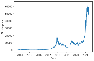 比特币价格走势
### 2.2 制作时间窗口
预期的数据格式为`[0,1,2,3,4,5,6] -> [7]`,即使用过去七天的价格预测接下来一天的价格。在此,使用TensorFlow提供的[timeseries_dataset_from_array](https://www.tensorflow.org/api_docs/python/tf/keras/utils/timeseries_dataset_from_array "timeseries_dataset_from_array") API进行窗口划分。
```python
timesteps = bitcoin_prices.index.to_numpy()
prices = bitcoin_prices["Price"].to_numpy()
HORIZON = 1 # 预测下一天的价格
WINDOW_SIZE = 7 # 基于过去7天的价格
input_data = prices[:-HORIZON]
targets = prices[WINDOW_SIZE:]
dataset = tf.keras.preprocessing.timeseries_dataset_from_array(
input_data, targets, sequence_length=WINDOW_SIZE)
for batch in dataset:
inputs, targets = batch
assert np.array_equal(inputs[0], prices[:WINDOW_SIZE])
assert np.array_equal(targets[0], prices[WINDOW_SIZE])
print(f"First Input:{inputs[0]}, Target:{targets[0]}")
print(f"Second Input:{inputs[1]}, Target:{targets[1]}")
break
```
返回如下,数据正确地转化成了预期的格式。
```python
First Input:[123.65499 125.455 108.58483 118.67466 121.33866 120.65533 121.795 ], Target:123.033
Second Input:[125.455 108.58483 118.67466 121.33866 120.65533 121.795 123.033 ], Target:124.049
```
### 2.3 分割数据
使用时间来划分训练集和验证集,仅做示例故不留测试集,实际中可按需操作。
```python
# tf.keras.preprocessing.timeseries_dataset_from_array返回的是batched dataset,所以先unbatch,方便分割数据
dataset = dataset.unbatch()
test_split = 0.2
split_index = int(len(list(dataset)) * (1-test_split))
# 分割完之后再分Batch,增加一维,不然无法满足模型数据维度要求
train_dataset = dataset.take(split_index).batch(batch_size=32)
test_dataset = dataset.skip(split_index).batch(batch_size=32)
```
## 3 建模
本文不追求极致的预测准确率,因此仅使用全连接层构建模型,代码如下:
```python
tf.random.set_seed(42)
tf.keras.backend.clear_session()
# 1. 构建模型
model = tf.keras.models.Sequential(
[
layers.Input(WINDOW_SIZE),
layers.Dense(128, activation="relu"),
layers.Dense(HORIZON, activation="linear")
]
, name="model_dense_base")
# 2. 编译模型
model.compile(loss='mae',
optimizer=tf.keras.optimizers.Adam(),
metrics=['mae'])
# 创建callback把表现最好的模型checkpoint存下来
def create_model_checkpoint(model_name, save_path="model_checkpoint"):
return tf.keras.callbacks.ModelCheckpoint(filepath=os.path.join(save_path, model_name),
verbose=0,
save_best_only=True)
# 3. 训练模型
model.fit( train_dataset,
epochs=100,
verbose=0,
validation_data=test_dataset,
callbacks=[create_model_checkpoint(model_name=model.name)]
)
```
将表现最好的模型加载回来做评估:
```python
model = tf.keras.models.load_model("model_checkpoint/model_dense_base")
model.evaluate(test_dataset)
```
返回如下,由平均绝对误差(MAE)可见预测的价格平均和真实价格相差700多美元。
```python
18/18 [==============================] - 1s 6ms/step - loss: 759.4327 - mae: 759.4327
[759.4326782226562, 759.4326782226562]
```
考虑到模型结构十分简单,结果有提升空间也在预期之内,根据本流程进行优化,完全可以预测得更准确。
## 4 总结
本文对单变量时间序列预测任务做了一个基准,其中TensorFlow的`tf.keras.preprocessing.timeseries_dataset_from_array`API简化了许多处理时间窗口的工作,之后将继续对TensorFlow预测时间序列的任务进行讨论。
## 5 相关阅读资料
- [Forecasting: Principles and Practice](https://otexts.com/fpp3/index.html)
比特币价格走势
### 2.2 制作时间窗口
预期的数据格式为`[0,1,2,3,4,5,6] -> [7]`,即使用过去七天的价格预测接下来一天的价格。在此,使用TensorFlow提供的[timeseries_dataset_from_array](https://www.tensorflow.org/api_docs/python/tf/keras/utils/timeseries_dataset_from_array "timeseries_dataset_from_array") API进行窗口划分。
```python
timesteps = bitcoin_prices.index.to_numpy()
prices = bitcoin_prices["Price"].to_numpy()
HORIZON = 1 # 预测下一天的价格
WINDOW_SIZE = 7 # 基于过去7天的价格
input_data = prices[:-HORIZON]
targets = prices[WINDOW_SIZE:]
dataset = tf.keras.preprocessing.timeseries_dataset_from_array(
input_data, targets, sequence_length=WINDOW_SIZE)
for batch in dataset:
inputs, targets = batch
assert np.array_equal(inputs[0], prices[:WINDOW_SIZE])
assert np.array_equal(targets[0], prices[WINDOW_SIZE])
print(f"First Input:{inputs[0]}, Target:{targets[0]}")
print(f"Second Input:{inputs[1]}, Target:{targets[1]}")
break
```
返回如下,数据正确地转化成了预期的格式。
```python
First Input:[123.65499 125.455 108.58483 118.67466 121.33866 120.65533 121.795 ], Target:123.033
Second Input:[125.455 108.58483 118.67466 121.33866 120.65533 121.795 123.033 ], Target:124.049
```
### 2.3 分割数据
使用时间来划分训练集和验证集,仅做示例故不留测试集,实际中可按需操作。
```python
# tf.keras.preprocessing.timeseries_dataset_from_array返回的是batched dataset,所以先unbatch,方便分割数据
dataset = dataset.unbatch()
test_split = 0.2
split_index = int(len(list(dataset)) * (1-test_split))
# 分割完之后再分Batch,增加一维,不然无法满足模型数据维度要求
train_dataset = dataset.take(split_index).batch(batch_size=32)
test_dataset = dataset.skip(split_index).batch(batch_size=32)
```
## 3 建模
本文不追求极致的预测准确率,因此仅使用全连接层构建模型,代码如下:
```python
tf.random.set_seed(42)
tf.keras.backend.clear_session()
# 1. 构建模型
model = tf.keras.models.Sequential(
[
layers.Input(WINDOW_SIZE),
layers.Dense(128, activation="relu"),
layers.Dense(HORIZON, activation="linear")
]
, name="model_dense_base")
# 2. 编译模型
model.compile(loss='mae',
optimizer=tf.keras.optimizers.Adam(),
metrics=['mae'])
# 创建callback把表现最好的模型checkpoint存下来
def create_model_checkpoint(model_name, save_path="model_checkpoint"):
return tf.keras.callbacks.ModelCheckpoint(filepath=os.path.join(save_path, model_name),
verbose=0,
save_best_only=True)
# 3. 训练模型
model.fit( train_dataset,
epochs=100,
verbose=0,
validation_data=test_dataset,
callbacks=[create_model_checkpoint(model_name=model.name)]
)
```
将表现最好的模型加载回来做评估:
```python
model = tf.keras.models.load_model("model_checkpoint/model_dense_base")
model.evaluate(test_dataset)
```
返回如下,由平均绝对误差(MAE)可见预测的价格平均和真实价格相差700多美元。
```python
18/18 [==============================] - 1s 6ms/step - loss: 759.4327 - mae: 759.4327
[759.4326782226562, 759.4326782226562]
```
考虑到模型结构十分简单,结果有提升空间也在预期之内,根据本流程进行优化,完全可以预测得更准确。
## 4 总结
本文对单变量时间序列预测任务做了一个基准,其中TensorFlow的`tf.keras.preprocessing.timeseries_dataset_from_array`API简化了许多处理时间窗口的工作,之后将继续对TensorFlow预测时间序列的任务进行讨论。
## 5 相关阅读资料
- [Forecasting: Principles and Practice](https://otexts.com/fpp3/index.html)
%20-%20Tail%20Pic.png)