Table of Contents
- Author(s) of this documentation:
- Bertrand Kerautret
Part of the Geometry package.
The Digital Straight Segment primitive (described here: Digital straight lines and segments) is commonly used to extract geometric information from digital contours. It is exploited in various estimators as for instance in tangent [75] or curvature estimation [67] . However, this primitive is not efficient to directly process real contours with the potential presence of noise. To overcome this limitation the alpha-thick segments (called initially Blurred Segments) were first introduced by Debled-Rennesson et al [48] which handle noise or contour irregularities.
We present here the recognition of alpha-thick segments as described in [48] and [51]. From a maximal thickness, it permits the recognition of a thick segment with the possibility to take into accounts some noise. Moreover the segment can be detected from points which are not necessarily connected nor necessarily digital points (RealPoint for instance).
- Note
- The proposed implementation is mainly a backport from ImaGene with some various refactoring.
Alpha-thick Segment
The first definition of blurred segment [48] relies on the definition of the digital straight lines (Digital straight lines and segments):
A set \( \mathcal{S}_f \) of consecutive points ( \( \mathcal{S}_f \geq 2 \)) of an 8-connected curve is a blurred segment with order \( d \) if there exists a discrete line \( \mathcal{D}(a,b, \mu, \omega) \) such that all points of \( \mathcal{S}_f \) belong to \( \mathcal{D} \) and \( \frac{\omega}{max(|a|,|b|)} \leq d \). The line \( D \) is said bounding for \( \mathcal{S}_f \).
Following this definition, the authors also propose an incremental linear time algorithm to segment a digital curve into blurred segments of order \( d \). The main drawback of such a decomposition is the non optimality (it implies over segmentation). Then the author introduce the notion of blurred segment of width \( \nu \) [47]. The width \( \nu \) is associated to the isothetic thickness of a set of points, ie. the minimum value between its vertical and horizontal thicknesses (see figure below).
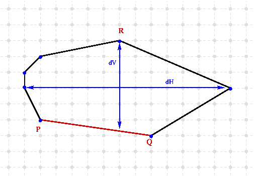
From this notion of isothetic thickness follows the blurred segment definition [47] :
A bounding line of a digital set \( \mathcal{S}_b \) is said optimal if its isothetic thickness is equal to the isothetic thickness of the convex hull \( conv(\mathcal{S}_b) \). \( \mathcal{S}_b \) is a blurred segment of width \( \nu \) if and only if its optimal bounding line has an isothetic distance less or equal to \( \nu \).
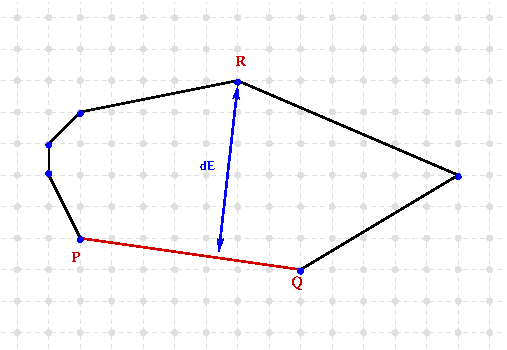
The implementation proposed here relies on the convex hull computed incrementally with the Melkman algorithm in linear time [93] (by using the MelkmanConvexHull class, see the module main documentation: Melkman's algorithm). It allows to add point on the front of the current segment and the value of vertical/horizontal thickness are computed in linear time by using the rotating caliper algorithm (see Convex hull thickness). The Buzer optimisation [88] to update the convex hull thickness with a coast of \(O(log\ n) \) or the linear time point subtraction are not yet implemented. Note that you can use also the Euclidean thickness (see illustration below) also defined from the rotating caliper algorithm.
Alpha-thick Segment Recognition
Type of Input Points
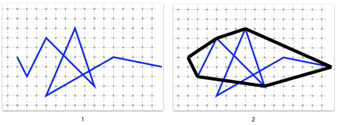
This implementation of the alpha-thick segments can take as input different types of points which just need to be given in the template parameter (TInputPoint). The input points are not necessary connected but the important constraint is that the sequence of point should not contains loop. Open or closed contours can be processed by the segment computer (if you use contour iterator in the initialisation you have just to check manually the end condition or the iterator type).
- Note
- Contrary to the implementation proposed in [47] the input points do not need to have axis increasing coordinates.
As illustration, the alpha-thick segments can be recognized on such contours:

And the example of non-simple contour can produce some errors:
Recognizing an Alpha-thick Segment
To recognize an alpha-thick segment, you need first to include the AlphaThickSegmentComputer header (with eventually the different namespace defined in StdDefs.h):
Afterwards, you have to set the type of the primitive by choosing the input point type. For instance, if you have to recognize input non digital points (e.g. Space::RealPoint), you can define:
To import an input contour you can use the the PointListReader class:
Then, you can define and initialize a new segment with maximal thickness set to 15:
- Note
- The maximal thickness given in initialization is by default the Vertical/horizontal thickness.
You can extend the segment by adding point to the front:
The final alpha-thick segment can also be displayed with a Board3D as other 2D geometric primitives:
As described in the Board3D documentation (Useful modes for several drawable elements), this primitive has two main display modes:
- default: the input point are displayed with its bounding box (the mode of the displayed points can also be changed).
- BoundingBox: only the bounding box is displayed.
You can also customize the segment color by using the CustomStyle object:
As illustration the segment recognition given in exampleAlphaThickSegmentNoisy.cpp produces such a display:
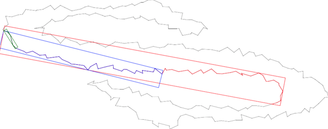
Other examples with other input types are given here: exampleAlphaThickSegment.cpp.
AlphaThickSegmentComputer with a point iterator
Since the AlphaThickSegmentComputer class is a model of CForwardSegmentComputer, you can initialize it from a given input point iterator. Then, the computer will not store the segment points (but the convexhull points are always stored). With such an initialization the segment computer can be used in a quite similar way as in the previous example:
Since the iterator is defined from an open contour, we check that we are not at the end of the input contour before applying any extension.
Changing the thickness definition
The thickness definition can be changed at the AlphaThickSegmentComputer construction:
Example of greedy segmentation into Alpha-thick Segment
To apply the greedy segmentation of a digital contour, we can use the GreedySegmentation class (since the AlphaThickSegmentComputer class is a model of the concept CForwardSegmentComputer):
The resulting set of segments can be displayed using the bounding box mode:
You should obtain such a visualization:
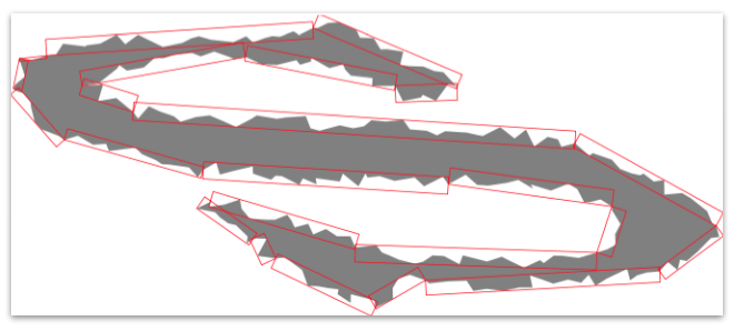
The whole example can be found in greedyAlphaThickDecomposition.cpp.
Computing AlphaThickSegment tangential cover
Tangential cover from saturated segmentation
To compute the tangential cover of a single contour, a first possibility is to use the SaturatedSegmentation class. As in the previous section, since the AlphaThickSegmentComputer is a model of the concept CForwardSegmentComputer, we can compute a saturated segmentation of the contour from maximal AlphaThickSegment (i.e a tangential cover) by using the SaturatedSegmentation class.
- See also
- This section is illustrated by using the example exampleAlphaThickSegmentTgtCover.cpp.
To obtain the complete tangential cover of a closed contour, we need to define a Circulator from the input contour. Thus, we have to include the the following headers:
Then, we can define this following types:
The contour Circulator is constructed from the a simple contour iterators:
The segmentation object can now be constructed as follows:
Finally we can access to the complete tangential cover and display it:
You will obtain such a resulting visualization:
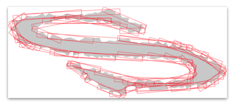
Tangential cover on a single point
Alternatively, if you only want the tangential cover associated to a single point, you can use the functions of the SegmentComputerUtils:
In particular, the function firstMaximalSegment and lastMaximalSegment permit to compute respectively the first and last maximal segment covering a particular point:
Then you will be able to access to all the maximal segments covering the point by using the function nextMaximalSegment :
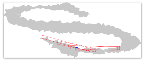
You will obtain for instance such a resulting cover:
