Table of Contents
- Author(s) of this documentation:
- Tristan Roussillon
Declaration
In this example, we show how to use the GridCurve object, which is key to analyze digital curves.
Using the Z2i shortcut, you can merely declare it as follows:
- Note
- The GridCurve object stands for an open or closed oriented grid curve, i.e. an alternating sequence of signed 0- and 1-cells.
Reading a grid curve from a file
You can load your grid curve from a text file that contains the coordinates of some points (each coordinate separated by a white space and one point per line).
For instance, the file smallSquare.dat used above contains:
Using the STL file stream, you can initialize your grid curve from the file data as follows:
- Note
- The coordinates of each point are assumed to be the digital coordinates of the 0-cells. These points are thus assumed to be 4-connected. The grid curve is assumed to be closed iff the first and last point are equal or 4-connected.
- A DGtal::IOException is raised in the case of IO errors and a DGtal::ConnectivityException is raised if the points are not 4-connected.
Displaying a grid curve with Board2D
DGtal::Board2D is a nice way of displaying many 2D objects.
See Board2D: a stream mechanism for displaying 2D digital objects for further details.
Using the stream mechanism of DGtal::Board2D, you can write your grid curve in a vector-graphics file (here in postscript, but xfig, svg, pdf are other available formats).
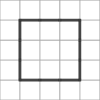
Here is a png conversion of the resulting image:

Ranges
A same digital curve may be viewed in very different ways:
either as an alternating sequence of cells, or as a sequence of points, or as a sequence of codes, and so one.
Moreover, some processing algorithms require a specific type of elements: either 4-connected points, 8-connected points, grid edges, and so one.
That is why the GridCurve object provides many ranges, i.e.
objects that provides services to iterate over a sequence of elements.
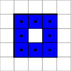
For instance, if you have to (or want to) work with 8-connected digital curves, you can get the grid curve inner points as follows:

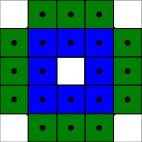
If you have to (or want to) work with separating algorithms, you can get the grid curve incident points as follows:

See GridCurve for the exhaustive list of available ranges and their basic usage. See Analysis of one-dimensional discrete structures for a general introduction about digital curves analysis.
Required includes
Here are the basic includes:
- Note
- StdDefs.h contains the Z2i namespace, which provides many type shortcuts. It includes the header required for the GridCurve object. ConfigExamples.h only provides the files sample path.
In order to use the drawing mechanism, you have to include: