library(datasets); data(swiss); require(stats); require(graphics)
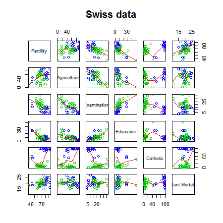
pairs(swiss, panel = panel.smooth, main = "Swiss data", col = 3 + (swiss$Catholic > 50))
Brian Caffo, Jeff Leek and Roger Peng
Johns Hopkins Bloomberg School of Public Health
library(datasets); data(swiss); require(stats); require(graphics)
pairs(swiss, panel = panel.smooth, main = "Swiss data", col = 3 + (swiss$Catholic > 50))

?swissStandardized fertility measure and socio-economic indicators for each of 47 French-speaking provinces of Switzerland at about 1888.
A data frame with 47 observations on 6 variables, each of which is in percent, i.e., in [0, 100].
All variables but ‘Fertility’ give proportions of the population.
lmsummary(lm(Fertility ~ . , data = swiss))
                 Estimate Std. Error t value  Pr(>|t|)
(Intercept)       66.9152   10.70604   6.250 1.906e-07
Agriculture       -0.1721    0.07030  -2.448 1.873e-02
Examination       -0.2580    0.25388  -1.016 3.155e-01
Education         -0.8709    0.18303  -4.758 2.431e-05
Catholic           0.1041    0.03526   2.953 5.190e-03
Infant.Mortality   1.0770    0.38172   2.822 7.336e-03
summary(lm(Fertility ~ Agriculture, data = swiss))$coefficients
            Estimate Std. Error t value  Pr(>|t|)
(Intercept)  60.3044    4.25126  14.185 3.216e-18
Agriculture   0.1942    0.07671   2.532 1.492e-02
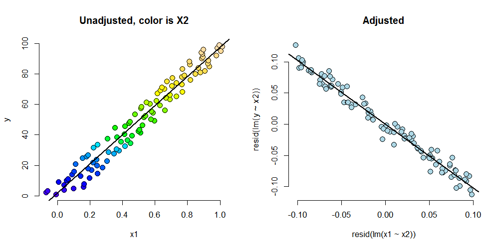
How can adjustment reverse the sign of an effect? Let's try a simulation.
n <- 100; x2 <- 1 : n; x1 <- .01 * x2 + runif(n, -.1, .1); y = -x1 + x2 + rnorm(n, sd = .01)
summary(lm(y ~ x1))$coef
            Estimate Std. Error t value  Pr(>|t|)
(Intercept)    1.618      1.200   1.349 1.806e-01
x1            95.854      2.058  46.579 1.153e-68
summary(lm(y ~ x1 + x2))$coef
              Estimate Std. Error   t value   Pr(>|t|)
(Intercept)  0.0003683  0.0020141    0.1829  8.553e-01
x1          -1.0215256  0.0166372  -61.4001  1.922e-79
x2           1.0001909  0.0001681 5950.1818 1.369e-271
z adds no new linear information, since it's a linear combination of variables already included. R just drops terms that are linear combinations of other terms.
z <- swiss$Agriculture + swiss$Education
lm(Fertility ~ . + z, data = swiss)
Call:
lm(formula = Fertility ~ . + z, data = swiss)

Coefficients:
     (Intercept)       Agriculture       Examination         Education          Catholic
          66.915            -0.172            -0.258            -0.871             0.104
Infant.Mortality                 z
           1.077                NA
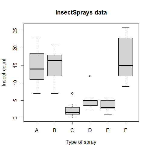
summary(lm(count ~ spray, data = InsectSprays))$coef
            Estimate Std. Error t value  Pr(>|t|)
(Intercept)  14.5000      1.132 12.8074 1.471e-19
sprayB        0.8333      1.601  0.5205 6.045e-01
sprayC      -12.4167      1.601 -7.7550 7.267e-11
sprayD       -9.5833      1.601 -5.9854 9.817e-08
sprayE      -11.0000      1.601 -6.8702 2.754e-09
sprayF        2.1667      1.601  1.3532 1.806e-01
summary(lm(count ~
             I(1 * (spray == 'B')) + I(1 * (spray == 'C')) +
             I(1 * (spray == 'D')) + I(1 * (spray == 'E')) +
             I(1 * (spray == 'F'))
           , data = InsectSprays))$coef
                      Estimate Std. Error t value  Pr(>|t|)
(Intercept)            14.5000      1.132 12.8074 1.471e-19
I(1 * (spray == "B"))   0.8333      1.601  0.5205 6.045e-01
I(1 * (spray == "C")) -12.4167      1.601 -7.7550 7.267e-11
I(1 * (spray == "D"))  -9.5833      1.601 -5.9854 9.817e-08
I(1 * (spray == "E")) -11.0000      1.601 -6.8702 2.754e-09
I(1 * (spray == "F"))   2.1667      1.601  1.3532 1.806e-01
lm(count ~
   I(1 * (spray == 'B')) + I(1 * (spray == 'C')) +
   I(1 * (spray == 'D')) + I(1 * (spray == 'E')) +
   I(1 * (spray == 'F')) + I(1 * (spray == 'A')), data = InsectSprays)
Call:
lm(formula = count ~ I(1 * (spray == "B")) + I(1 * (spray ==
    "C")) + I(1 * (spray == "D")) + I(1 * (spray == "E")) + I(1 *
    (spray == "F")) + I(1 * (spray == "A")), data = InsectSprays)

Coefficients:
          (Intercept)  I(1 * (spray == "B"))  I(1 * (spray == "C"))  I(1 * (spray == "D"))
               14.500                  0.833                -12.417                 -9.583
I(1 * (spray == "E"))  I(1 * (spray == "F"))  I(1 * (spray == "A"))
              -11.000                  2.167                     NA
summary(lm(count ~ spray - 1, data = InsectSprays))$coef
       Estimate Std. Error t value  Pr(>|t|)
sprayA   14.500      1.132  12.807 1.471e-19
sprayB   15.333      1.132  13.543 1.002e-20
sprayC    2.083      1.132   1.840 7.024e-02
sprayD    4.917      1.132   4.343 4.953e-05
sprayE    3.500      1.132   3.091 2.917e-03
sprayF   16.667      1.132  14.721 1.573e-22
unique(ave(InsectSprays$count, InsectSprays$spray))
[1] 14.500 15.333 2.083 4.917 3.500 16.667
spray2 <- relevel(InsectSprays$spray, "C")
summary(lm(count ~ spray2, data = InsectSprays))$coef
            Estimate Std. Error t value  Pr(>|t|)
(Intercept)    2.083      1.132  1.8401 7.024e-02
spray2A       12.417      1.601  7.7550 7.267e-11
spray2B       13.250      1.601  8.2755 8.510e-12
spray2D        2.833      1.601  1.7696 8.141e-02
spray2E        1.417      1.601  0.8848 3.795e-01
spray2F       14.583      1.601  9.1083 2.794e-13
Equivalently \[Var(\hat \beta_B - \hat \beta_C) = Var(\hat \beta_B) + Var(\hat \beta_C) - 2 Cov(\hat \beta_B, \hat \beta_C)\]
fit <- lm(count ~ spray, data = InsectSprays) #A is ref
bbmbc <- coef(fit)[2] - coef(fit)[3] #B - C
temp <- summary(fit)
se <- temp$sigma * sqrt(temp$cov.unscaled[2, 2] + temp$cov.unscaled[3,3] - 2 *temp$cov.unscaled[2,3])
t <- (bbmbc) / se
p <- pt(-abs(t), df = fit$df)
out <- c(bbmbc, se, t, p)
names(out) <- c("B - C", "SE", "T", "P")
round(out, 3)
 B - C     SE      T      P
13.250  1.601  8.276  0.000
http://www.un.org/millenniumgoals/pdf/MDG_FS_1_EN.pdf
http://apps.who.int/gho/athena/data/GHO/WHOSIS_000008.csv?profile=text&filter=COUNTRY:;SEX:
#download.file("http://apps.who.int/gho/athena/data/GHO/WHOSIS_000008.csv?profile=text&filter=COUNTRY:*;SEX:*","hunger.csv",method="curl")
hunger <- read.csv("hunger.csv")
hunger <- hunger[hunger$Sex!="Both sexes",]
head(hunger)
                               Indicator Data.Source PUBLISH.STATES Year            WHO.region
1 Children aged <5 years underweight (%) NLIS_310044      Published 1986                Africa
2 Children aged <5 years underweight (%) NLIS_310233      Published 1990              Americas
3 Children aged <5 years underweight (%) NLIS_312902      Published 2005              Americas
5 Children aged <5 years underweight (%) NLIS_312522      Published 2002 Eastern Mediterranean
6 Children aged <5 years underweight (%) NLIS_312955      Published 2008                Africa
8 Children aged <5 years underweight (%) NLIS_312963      Published 2008                Africa
        Country    Sex Display.Value Numeric Low High Comments
1       Senegal   Male          19.3    19.3  NA   NA       NA
2      Paraguay   Male           2.2     2.2  NA   NA       NA
3     Nicaragua   Male           5.3     5.3  NA   NA       NA
5        Jordan Female           3.2     3.2  NA   NA       NA
6 Guinea-Bissau Female          17.0    17.0  NA   NA       NA
8         Ghana   Male          15.7    15.7  NA   NA       NA
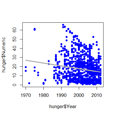
lm1 <- lm(hunger$Numeric ~ hunger$Year)
plot(hunger$Year,hunger$Numeric,pch=19,col="blue")
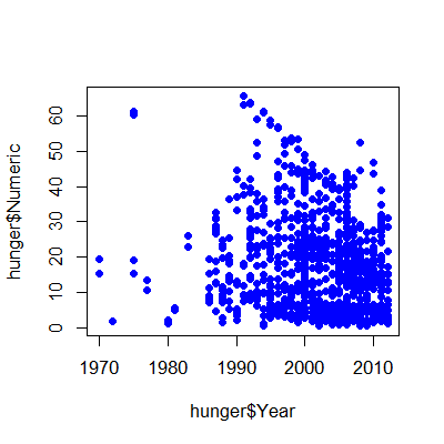
\[Hu_i = b_0 + b_1 Y_i + e_i\]
\(b_0\) = percent hungry at Year 0
\(b_1\) = decrease in percent hungry per year
\(e_i\) = everything we didn't measure
lm1 <- lm(hunger$Numeric ~ hunger$Year)
plot(hunger$Year,hunger$Numeric,pch=19,col="blue")
lines(hunger$Year,lm1$fitted,lwd=3,col="darkgrey")
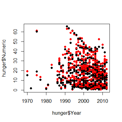
plot(hunger$Year,hunger$Numeric,pch=19)
points(hunger$Year,hunger$Numeric,pch=19,col=((hunger$Sex=="Male")*1+1))
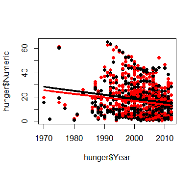
\[HuF_i = bf_0 + bf_1 YF_i + ef_i\]
\(bf_0\) = percent of girls hungry at Year 0
\(bf_1\) = decrease in percent of girls hungry per year
\(ef_i\) = everything we didn't measure
\[HuM_i = bm_0 + bm_1 YM_i + em_i\]
\(bm_0\) = percent of boys hungry at Year 0
\(bm_1\) = decrease in percent of boys hungry per year
\(em_i\) = everything we didn't measure
lmM <- lm(hunger$Numeric[hunger$Sex=="Male"] ~ hunger$Year[hunger$Sex=="Male"])
lmF <- lm(hunger$Numeric[hunger$Sex=="Female"] ~ hunger$Year[hunger$Sex=="Female"])
plot(hunger$Year,hunger$Numeric,pch=19)
points(hunger$Year,hunger$Numeric,pch=19,col=((hunger$Sex=="Male")*1+1))
lines(hunger$Year[hunger$Sex=="Male"],lmM$fitted,col="black",lwd=3)
lines(hunger$Year[hunger$Sex=="Female"],lmF$fitted,col="red",lwd=3)
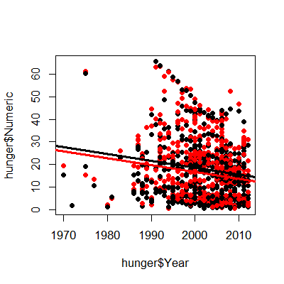
\[Hu_i = b_0 + b_1 \mathbb{1}(Sex_i="Male") + b_2 Y_i + e^*_i\]
\(b_0\) - percent hungry at year zero for females
\(b_0 + b_1\) - percent hungry at year zero for males
\(b_2\) - change in percent hungry (for either males or females) in one year
\(e^*_i\) - everything we didn't measure
lmBoth <- lm(hunger$Numeric ~ hunger$Year + hunger$Sex)
plot(hunger$Year,hunger$Numeric,pch=19)
points(hunger$Year,hunger$Numeric,pch=19,col=((hunger$Sex=="Male")*1+1))
abline(c(lmBoth$coeff[1],lmBoth$coeff[2]),col="red",lwd=3)
abline(c(lmBoth$coeff[1] + lmBoth$coeff[3],lmBoth$coeff[2] ),col="black",lwd=3)
\[Hu_i = b_0 + b_1 \mathbb{1}(Sex_i="Male") + b_2 Y_i + b_3 \mathbb{1}(Sex_i="Male")\times Y_i + e^+_i\]
\(b_0\) - percent hungry at year zero for females
\(b_0 + b_1\) - percent hungry at year zero for males
\(b_2\) - change in percent hungry (females) in one year
\(b_2 + b_3\) - change in percent hungry (males) in one year
\(e^+_i\) - everything we didn't measure
lmBoth <- lm(hunger$Numeric ~ hunger$Year + hunger$Sex + hunger$Sex*hunger$Year)
plot(hunger$Year,hunger$Numeric,pch=19)
points(hunger$Year,hunger$Numeric,pch=19,col=((hunger$Sex=="Male")*1+1))
abline(c(lmBoth$coeff[1],lmBoth$coeff[2]),col="red",lwd=3)
abline(c(lmBoth$coeff[1] + lmBoth$coeff[3],lmBoth$coeff[2] +lmBoth$coeff[4]),col="black",lwd=3)
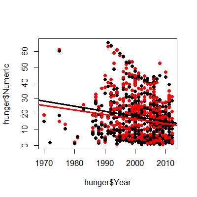
summary(lmBoth)
Call:
lm(formula = hunger$Numeric ~ hunger$Year + hunger$Sex + hunger$Sex *
    hunger$Year)

Residuals:
   Min     1Q Median     3Q    Max
-25.91 -11.25  -1.85   7.09  46.15

Coefficients:
                           Estimate Std. Error t value Pr(>|t|)
(Intercept)                603.5058   171.0552    3.53  0.00044 ***
hunger$Year                 -0.2934     0.0855   -3.43  0.00062 ***
hunger$SexMale              61.9477   241.9086    0.26  0.79795
hunger$Year:hunger$SexMale  -0.0300     0.1209   -0.25  0.80402
---
Signif. codes:  0 '***' 0.001 '**' 0.01 '*' 0.05 '.' 0.1 ' ' 1

Residual standard error: 13.2 on 944 degrees of freedom
Multiple R-squared:  0.0318,    Adjusted R-squared:  0.0287
F-statistic: 10.3 on 3 and 944 DF,  p-value: 1.06e-06
\[ E[Y_i | X_{1i}=x_1, X_{2i}=x_2] = \beta_0 + \beta_1 x_{1} + \beta_2 x_{2} + \beta_3 x_{1}x_{2} \] Holding \(X_2\) constant we have \[ E[Y_i | X_{1i}=x_1+1, X_{2i}=x_2]-E[Y_i | X_{1i}=x_1, X_{2i}=x_2] = \beta_1 + \beta_3 x_{2} \] And thus the expected change in \(Y\) per unit change in \(X_1\) holding all else constant is not constant. \(\beta_1\) is the slope when \(x_{2} = 0\). Note further that: \[ E[Y_i | X_{1i}=x_1+1, X_{2i}=x_2+1]-E[Y_i | X_{1i}=x_1, X_{2i}=x_2+1] \] \[ -E[Y_i | X_{1i}=x_1+1, X_{2i}=x_2]-E[Y_i | X_{1i}=x_1, X_{2i}=x_2] \] \[ =\beta_3 \] Thus, \(\beta_3\) is the change in the expected change in \(Y\) per unit change in \(X_1\), per unit change in \(X_2\).
Or, the change in the slope relating \(X_1\) and \(Y\) per unit change in \(X_2\).
\[Hu_i = b_0 + b_1 In_i + b_2 Y_i + b_3 In_i \times Y_i + e^+_i\]
\(b_0\) - percent hungry at year zero for children with whose parents have no income
\(b_1\) - change in percent hungry for each dollar of income in year zero
\(b_2\) - change in percent hungry in one year for children whose parents have no income
\(b_3\) - increased change in percent hungry by year for each dollar of income - e.g. if income is $10,000, then change in percent hungry in one year will be
\[b_2 + 1e4 \times b_3\]
\(e^+_i\) - everything we didn't measure
Lot's of care/caution needed!