What is a density surface model?
================================
css: custom.css
transition: none
```{r setup, include=FALSE}
# setup
library(knitr)
library(magrittr)
library(viridis)
opts_chunk$set(cache=TRUE, echo=FALSE, out.width='\\textwidth', fig.height=10, fig.width=10)
```
Why model abundance spatially?
==============================
- Use non-designed surveys
- Use environmental information
- Maps
Back to Horvitz-Thompson estimation
===================================
type:section
Horvitz-Thompson-like estimators
================================
- Rescale the (flat) density and extrapolate
$$
\hat{N} = \frac{\text{study area}}{\text{covered area}}\sum_{i=1}^n \frac{s_i}{\hat{p}_i}
$$
- $s_i$ are group/cluster sizes
- $\hat{p}_i$ is the detection probability (from detection function)
Hidden in this formula is a simple assumption
=============================================
- Probability of sampling every point in the study area is equal
- Is this true? Sometimes.
- If (and only if) the design is randomised
Many faces of randomisation
===========================
```{r randomisation, fig.width=14, fig.height=4.5, out.width='\\textwidth'}
set.seed(12133)
par(mfrow=c(1,3), cex.main=2.5)
# true random sample
plot(c(0, 1), c(0, 1), type="n", xlab="", ylab="", axes=FALSE, asp=1, main="random placement")
dat <- data.frame(x=runif(10), y=runif(10))
angle <- runif(10, 0, 2*pi)
len <- 0.2
arrows(dat$x, dat$y, dat$x+len*cos(angle), dat$y+len*sin(angle), length=0)
dat <- data.frame(x=runif(10), y=runif(10))
angle <- runif(10, 0, 2*pi)
len <- 0.2
arrows(dat$x, dat$y, dat$x+len*cos(angle), dat$y+len*sin(angle), length=0, col="grey40", lty=2)
box()
# parallel random offset
plot(c(0, 1), c(0, 1), type="n", xlab="", ylab="", axes=FALSE, asp=1, main="random offset parallel lines")
abline(v=seq(0, 1, len=10))
abline(v=seq(0, 1, len=10)+0.07, col="grey40", lty=2)
box()
# random offset zigzag
## make a zigzag
n_segs <- 10
zz <- data.frame(x = c(seq(0, 0.5, len=n_segs),
seq(0.5, 1, len=n_segs)),
y = c(seq(0, 1, len=n_segs),
seq(1, 0, len=n_segs)))
# many zigzags
mzz <- rbind(zz,zz,zz)
mzz$x <- mzz$x/3
ind <- 1:nrow(zz)
mzz$x[ind+nrow(zz)] <- mzz$x[ind+nrow(zz)]+1/3
mzz$x[ind+2*nrow(zz)] <- mzz$x[ind+2*nrow(zz)]+2/3
plot(mzz, type="l", xlab="", ylab="", axes=FALSE, asp=1, main="random offset zigzag")
lines(mzz$x+0.06, mzz$y, col="grey40", lty=2)
box()
```
Randomisation & coverage probability
=====================================
- H-T equation above assumes even coverage
- (or you can estimate)
 Extra information
========================================================
```{r loadtracks, results="hide"}
library(rgdal)
tracksEN <- readOGR("../spermwhaledata/rawdata/Analysis.gdb", "EN_Trackline1")
tracksGU <- readOGR("../spermwhaledata/rawdata/Analysis.gdb", "GU_Trackline")
```
```{r plottracks, cache=FALSE}
library(ggplot2)
tracksEN <- fortify(tracksEN)
tracksGU <- fortify(tracksGU)
mapdata <- map_data("world2","usa")
p_maptr <- ggplot()+
geom_path(aes(x=long,y=lat, group=group), colour="red", data=tracksEN) +
geom_path(aes(x=long,y=lat, group=group), colour="blue", data=tracksGU)+
geom_polygon(aes(x=long,y=lat, group=group), data=mapdata)+
theme_minimal() +
coord_map(xlim=range(tracksEN$long, tracksGU$long)+c(-1,1),
ylim=range(tracksEN$lat, tracksGU$lat)+c(-1,1))
print(p_maptr)
```
Extra information - depth
==========================
```{r loadcovars, results="hide"}
library(raster)
predictorStack <- stack(c("../spermwhaledata/rawdata/Covariates_for_Study_Area/Depth.img", "../spermwhaledata/rawdata/Covariates_for_Study_Area/GLOB/CMC/CMC0.2deg/analysed_sst/2004/20040601-CMC-L4SSTfnd-GLOB-v02-fv02.0-CMC0.2deg-analysed_sst.img","../spermwhaledata/rawdata/Covariates_for_Study_Area/VGPM/Rasters/vgpm.2004153.hdf.gz.img"))
names(predictorStack) <- c("Depth","SST","NPP")
```
```{r plotdepth}
load("../spermwhaledata/R_import/spermwhale.RData")
depthdat <- as.data.frame(predictorStack[[1]],xy=TRUE)
depthdat <- depthdat[!is.na(depthdat$Depth),]
library(plyr)
plotobs <- join(obs, segs, by="Sample.Label")
p <- ggplot() +
geom_tile(aes(x=x, y=y, fill=Depth), data=depthdat) +
geom_point(aes(x=x, y=y, size=size), alpha=0.6, data=plotobs) +
coord_equal() +
scale_fill_viridis() +
theme_minimal()
print(p)
```
Extra information - depth
==========================
```{r plotdepth-notspat, fig.width=10}
p <- ggplot(plotobs)+
geom_histogram(aes(Depth, weight=size)) +
xlab("Depth") + ylab("Aggregated counts") +
theme_minimal()
print(p)
```
***
- NB this only shows segments where counts > 0
Extra information - SST
============================================
```{r plotsst, fig.width=10}
sstdat <- as.data.frame(predictorStack[[2]], xy=TRUE)
sstdat <- sstdat[!is.na(sstdat$SST),]
p <- ggplot() +
geom_tile(aes(x=x, y=y, fill=SST), data=sstdat) +
geom_point(aes(x=x, y=y, size=size), alpha=0.6, data=plotobs) +
coord_equal() + scale_fill_viridis() +
theme_minimal()
print(p)
```
Extra information - SST
============================================
```{r plotsst-notspat, fig.width=10}
p <- ggplot(plotobs)+
geom_histogram(aes(SST, weight=size), binwidth=1) +
xlab("SST") + ylab("Aggregated counts") +
theme_minimal()
print(p)
```
***
- (only segments where counts > 0)
You should model that
=====================
type: section
Modelling outputs
===================
- Abundance and uncertainty
- Arbitrary areas
- Numeric values
- Maps
- Extrapolation (with caution!)
- Covariate effects
- count/sample as function of covars
Modelling requirements
========================
- Include detectability
- Account for effort
- Flexible/interpretable effects
- Predictions over an arbitrary area
Accounting for effort
======================
type:section
Effort
==========
```{r tracks2, fig.width=10}
print(p_maptr)
```
***
- Have transects
- Variation in counts and covars along them
- Want a sample unit w/ minimal variation
- "Segments": chunks of effort
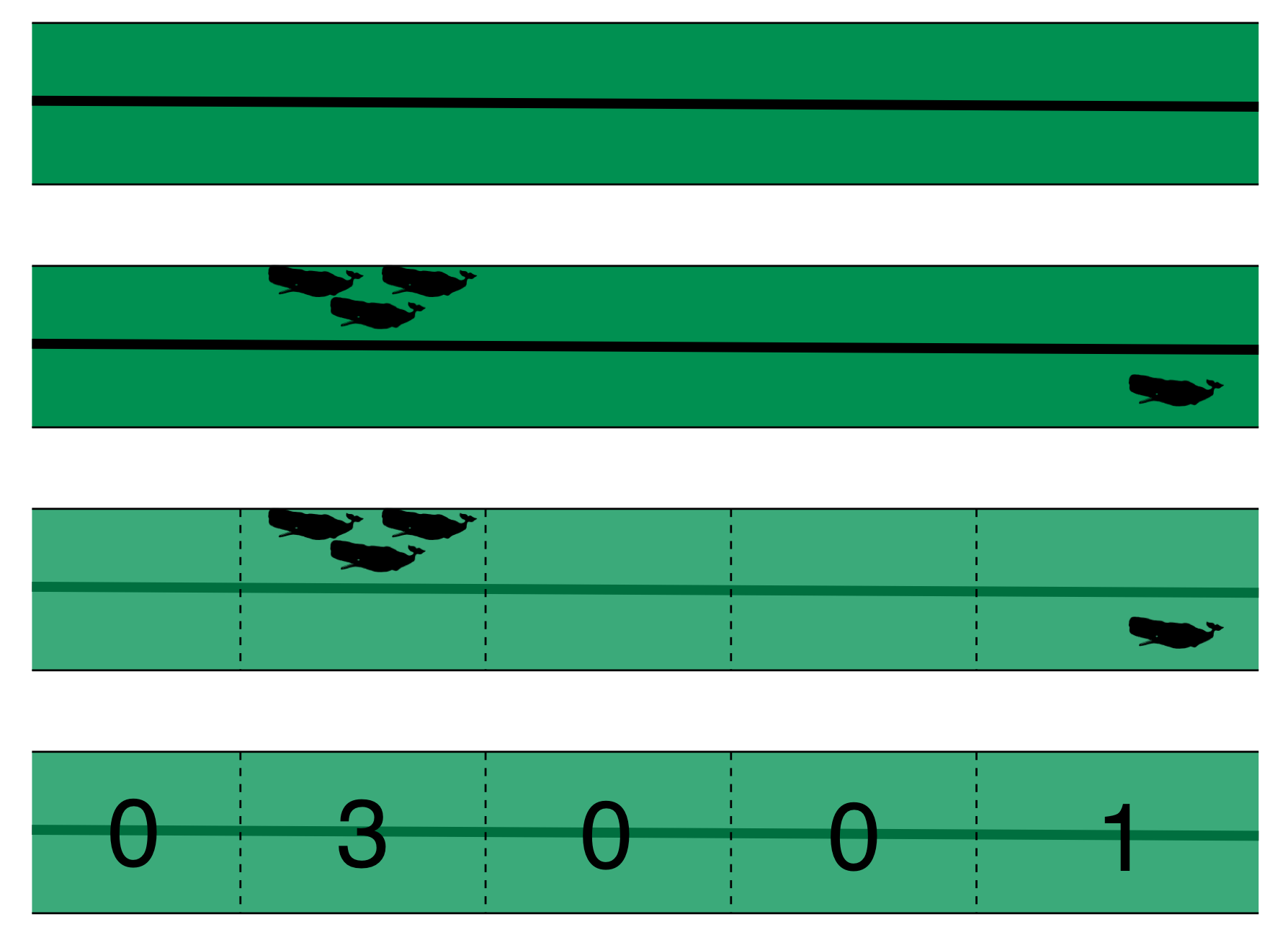
Chopping up transects
======================
Extra information
========================================================
```{r loadtracks, results="hide"}
library(rgdal)
tracksEN <- readOGR("../spermwhaledata/rawdata/Analysis.gdb", "EN_Trackline1")
tracksGU <- readOGR("../spermwhaledata/rawdata/Analysis.gdb", "GU_Trackline")
```
```{r plottracks, cache=FALSE}
library(ggplot2)
tracksEN <- fortify(tracksEN)
tracksGU <- fortify(tracksGU)
mapdata <- map_data("world2","usa")
p_maptr <- ggplot()+
geom_path(aes(x=long,y=lat, group=group), colour="red", data=tracksEN) +
geom_path(aes(x=long,y=lat, group=group), colour="blue", data=tracksGU)+
geom_polygon(aes(x=long,y=lat, group=group), data=mapdata)+
theme_minimal() +
coord_map(xlim=range(tracksEN$long, tracksGU$long)+c(-1,1),
ylim=range(tracksEN$lat, tracksGU$lat)+c(-1,1))
print(p_maptr)
```
Extra information - depth
==========================
```{r loadcovars, results="hide"}
library(raster)
predictorStack <- stack(c("../spermwhaledata/rawdata/Covariates_for_Study_Area/Depth.img", "../spermwhaledata/rawdata/Covariates_for_Study_Area/GLOB/CMC/CMC0.2deg/analysed_sst/2004/20040601-CMC-L4SSTfnd-GLOB-v02-fv02.0-CMC0.2deg-analysed_sst.img","../spermwhaledata/rawdata/Covariates_for_Study_Area/VGPM/Rasters/vgpm.2004153.hdf.gz.img"))
names(predictorStack) <- c("Depth","SST","NPP")
```
```{r plotdepth}
load("../spermwhaledata/R_import/spermwhale.RData")
depthdat <- as.data.frame(predictorStack[[1]],xy=TRUE)
depthdat <- depthdat[!is.na(depthdat$Depth),]
library(plyr)
plotobs <- join(obs, segs, by="Sample.Label")
p <- ggplot() +
geom_tile(aes(x=x, y=y, fill=Depth), data=depthdat) +
geom_point(aes(x=x, y=y, size=size), alpha=0.6, data=plotobs) +
coord_equal() +
scale_fill_viridis() +
theme_minimal()
print(p)
```
Extra information - depth
==========================
```{r plotdepth-notspat, fig.width=10}
p <- ggplot(plotobs)+
geom_histogram(aes(Depth, weight=size)) +
xlab("Depth") + ylab("Aggregated counts") +
theme_minimal()
print(p)
```
***
- NB this only shows segments where counts > 0
Extra information - SST
============================================
```{r plotsst, fig.width=10}
sstdat <- as.data.frame(predictorStack[[2]], xy=TRUE)
sstdat <- sstdat[!is.na(sstdat$SST),]
p <- ggplot() +
geom_tile(aes(x=x, y=y, fill=SST), data=sstdat) +
geom_point(aes(x=x, y=y, size=size), alpha=0.6, data=plotobs) +
coord_equal() + scale_fill_viridis() +
theme_minimal()
print(p)
```
Extra information - SST
============================================
```{r plotsst-notspat, fig.width=10}
p <- ggplot(plotobs)+
geom_histogram(aes(SST, weight=size), binwidth=1) +
xlab("SST") + ylab("Aggregated counts") +
theme_minimal()
print(p)
```
***
- (only segments where counts > 0)
You should model that
=====================
type: section
Modelling outputs
===================
- Abundance and uncertainty
- Arbitrary areas
- Numeric values
- Maps
- Extrapolation (with caution!)
- Covariate effects
- count/sample as function of covars
Modelling requirements
========================
- Include detectability
- Account for effort
- Flexible/interpretable effects
- Predictions over an arbitrary area
Accounting for effort
======================
type:section
Effort
==========
```{r tracks2, fig.width=10}
print(p_maptr)
```
***
- Have transects
- Variation in counts and covars along them
- Want a sample unit w/ minimal variation
- "Segments": chunks of effort
Chopping up transects
======================
 [Physeter catodon by Noah Schlottman](http://phylopic.org/image/dc76cbdb-dba5-4d8f-8cf3-809515c30dbd/)
Flexible, interpretable effects
================================
type:section
Smooth response
================
```{r plotsmooths, messages=FALSE}
library(Distance)
library(dsm)
df <- ds(dist, truncation=6000)
dsm_tw_xy_depth <- dsm(count ~ s(x, y) + s(Depth), ddf.obj=df, observation.data=obs, segment.data=segs, family=tw())
plot(dsm_tw_xy_depth, select=2)
```
Explicit spatial effects
============================
```{r plot-spat-smooths, messages=FALSE}
vis.gam(dsm_tw_xy_depth, view=c("x","y"), plot.type="contour", main="", asp=1, too.far=0.06)
```
Predictions
================================
type:section
Predictions over an arbitrary area
===================================
```{r predplot}
predgrid$Nhat <- predict(dsm_tw_xy_depth, predgrid)
p <- ggplot(predgrid) +
geom_tile(aes(x=x, y=y, fill=Nhat, width=10*1000, height=10*1000)) +
coord_equal() +
labs(fill="Density") +
scale_fill_viridis() +
theme_minimal()
print(p)
```
***
- Don't want to be restricted to predict on segments
- Predict within survey area
- Extrapolate outside (with caution)
- Working on a grid of cells
Detection information
================================
type:section
Including detection information
=================================
- Two options:
- adjust areas to account for **effective effort**
- use **Horvitz-Thompson estimates** as response
Effective effort
================
- Area of each segment, $A_j$
- use $A_j\hat{p}_j$
- think effective strip width ($\hat{\mu} = w\hat{p}$)
- Response is counts per segment
- "Adjusting for effort"
- "Count model"
Estimated abundance
===================
- Estimate H-T abundance per segment
- Effort is area of each segment
- "Estimated abundance" per segment
$$
\hat{n}_j = \sum_{i \text{ in segment } j } \frac{s_i}{\hat{p}_i}
$$
Detectability and covariates
=============================
- 2 covariate "levels" in detection function
- "Observer"/"observation" -- change **within** segment
- "Segment" -- change **between** segments
- "Count model" only lets us use segment-level covariates
- "Estimated abundance" lets us use either
When to use each approach?
============================
- Generally "nicer" to adjust effort
- Keep response (counts) close to what was observed
- **Unless** you want observation-level covariates
- These *can* make a big difference!
Availability, perception bias and more
=============================
- $\hat{p}$ is not always simple!
- Availability & perception bias somehow enter
- We can make explicit models for this
- More later in the course
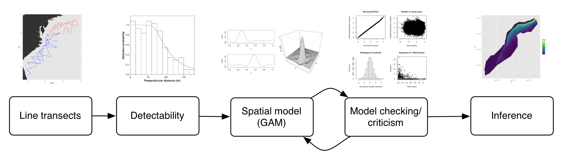
DSM flow diagram
==================
[Physeter catodon by Noah Schlottman](http://phylopic.org/image/dc76cbdb-dba5-4d8f-8cf3-809515c30dbd/)
Flexible, interpretable effects
================================
type:section
Smooth response
================
```{r plotsmooths, messages=FALSE}
library(Distance)
library(dsm)
df <- ds(dist, truncation=6000)
dsm_tw_xy_depth <- dsm(count ~ s(x, y) + s(Depth), ddf.obj=df, observation.data=obs, segment.data=segs, family=tw())
plot(dsm_tw_xy_depth, select=2)
```
Explicit spatial effects
============================
```{r plot-spat-smooths, messages=FALSE}
vis.gam(dsm_tw_xy_depth, view=c("x","y"), plot.type="contour", main="", asp=1, too.far=0.06)
```
Predictions
================================
type:section
Predictions over an arbitrary area
===================================
```{r predplot}
predgrid$Nhat <- predict(dsm_tw_xy_depth, predgrid)
p <- ggplot(predgrid) +
geom_tile(aes(x=x, y=y, fill=Nhat, width=10*1000, height=10*1000)) +
coord_equal() +
labs(fill="Density") +
scale_fill_viridis() +
theme_minimal()
print(p)
```
***
- Don't want to be restricted to predict on segments
- Predict within survey area
- Extrapolate outside (with caution)
- Working on a grid of cells
Detection information
================================
type:section
Including detection information
=================================
- Two options:
- adjust areas to account for **effective effort**
- use **Horvitz-Thompson estimates** as response
Effective effort
================
- Area of each segment, $A_j$
- use $A_j\hat{p}_j$
- think effective strip width ($\hat{\mu} = w\hat{p}$)
- Response is counts per segment
- "Adjusting for effort"
- "Count model"
Estimated abundance
===================
- Estimate H-T abundance per segment
- Effort is area of each segment
- "Estimated abundance" per segment
$$
\hat{n}_j = \sum_{i \text{ in segment } j } \frac{s_i}{\hat{p}_i}
$$
Detectability and covariates
=============================
- 2 covariate "levels" in detection function
- "Observer"/"observation" -- change **within** segment
- "Segment" -- change **between** segments
- "Count model" only lets us use segment-level covariates
- "Estimated abundance" lets us use either
When to use each approach?
============================
- Generally "nicer" to adjust effort
- Keep response (counts) close to what was observed
- **Unless** you want observation-level covariates
- These *can* make a big difference!
Availability, perception bias and more
=============================
- $\hat{p}$ is not always simple!
- Availability & perception bias somehow enter
- We can make explicit models for this
- More later in the course
DSM flow diagram
==================
 Spatial models
===============
type: section
Abundance as a function of covariates
=======================================
- Two approaches to model abundance
- Explicit spatial models
- When: good coverage, fixed area
- "Habitat" models (no explicit spatial terms)
- When: poorer coverage, extrapolation
- We'll cover both approaches here
Data requirements
=====================================
type:section
What do we need?
===================
- Need to "link" data
- Distance data/detection function
- Segment data
- Observation data to link segments to detections
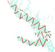
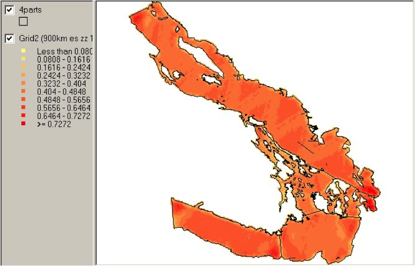
Example of spatial data in QGIS
=====================================
type:section
Recap
======
- Model counts or estimated abundace
- The effort is accounted for differently
- Flexible models are good
- Incorporate detectability
- 2 tables + detection function needed
Spatial models
===============
type: section
Abundance as a function of covariates
=======================================
- Two approaches to model abundance
- Explicit spatial models
- When: good coverage, fixed area
- "Habitat" models (no explicit spatial terms)
- When: poorer coverage, extrapolation
- We'll cover both approaches here
Data requirements
=====================================
type:section
What do we need?
===================
- Need to "link" data
- Distance data/detection function
- Segment data
- Observation data to link segments to detections
Example of spatial data in QGIS
=====================================
type:section
Recap
======
- Model counts or estimated abundace
- The effort is accounted for differently
- Flexible models are good
- Incorporate detectability
- 2 tables + detection function needed