Model checking
===============
css: custom.css
transition: none
```{r setup, include=FALSE}
library(knitr)
library(magrittr)
library(viridis)
library(ggplot2)
library(reshape2)
library(animation)
opts_chunk$set(cache=TRUE, echo=FALSE, fig.height=10, fig.width=10)
```
```{r initialmodeletc, echo=FALSE, message=FALSE, warning=FALSE}
load("../spermwhaledata/R_import/spermwhale.RData")
library(Distance)
library(dsm)
df <- ds(dist, truncation=6000)
dsm_tw_xy_depth <- dsm(count ~ s(x, y) + s(Depth), ddf.obj=df, observation.data=obs, segment.data=segs, family=tw())
dsm_x_tw <- dsm(count~s(x), ddf.obj=df,
segment.data=segs, observation.data=obs,
family=tw())
```
intro
======
type:section
title:none
*"perhaps the most important part of applied statistical modelling"*
Simon Wood
Model checking
===============
- Checking $\neq$ validation!
- As with detection function, checking is important
- Want to know the model conforms to assumptions
- What assumptions should we check?
What to check
===============
- Convergence
- Basis size
- Residuals
Convergence
===========
type:section
Convergence
===========
- Fitting the GAM involves an optimization
- By default this is REstricted Maximum Likelihood (REML) score
- Sometimes this can go wrong
- R will warn you!
A model that converges
======================
```{r convcheck, echo=TRUE, fig.keep="none"}
gam.check(dsm_tw_xy_depth)
```
A bad model
===========
```
Error in while (mean(ldxx/(ldxx + ldss)) > 0.4) { :
missing value where TRUE/FALSE needed
In addition: Warning message:
In sqrt(w) : NaNs produced
Error in while (mean(ldxx/(ldxx + ldss)) > 0.4) { :
missing value where TRUE/FALSE needed
```
This is **rare**
The Folk Theorem of Statistical Computing
============
type:section
"most statistical computational problems are due not to the algorithm being used but rather the model itself"
Andrew Gelman
Basis size
===========
type:section
Basis size (k)
===========
- Set `k` per term
- e.g. `s(x, k=10)` or `s(x, y, k=100)`
- Penalty removes "extra" wigglyness
- *up to a point!*
- (But computation is slower with bigger `k`)
Checking basis size
====================
```{r gamcheck-text, fig.keep="none", echo=TRUE}
gam.check(dsm_x_tw)
```
Increasing basis size
====================
```{r gamcheck-kplus-text, fig.keep="none", echo=TRUE}
dsm_x_tw_k <- dsm(count~s(x, k=20), ddf.obj=df,
segment.data=segs, observation.data=obs,
family=tw())
gam.check(dsm_x_tw_k)
```
Sometimes basis size isn't the issue...
========================================
- Generally, double `k` and see what happens
- Didn't increase the EDF much here
- Other things can cause low "`p-value`" and "`k-index`"
- Increasing `k` can cause problems (nullspace)
k is a maximum
==============
- (Usually) Don't need to worry about things being too wiggly
- `k` gives the maximum complexity
- Penalty deals with the rest
```{r plotk, fig.width=18, fig.height=9 }
dsm_sst_k5 <- dsm(count~s(SST, k=5), ddf.obj=df,
segment.data=segs, observation.data=obs,
family=tw())
dsm_sst_k20 <- dsm(count~s(SST, k=20), ddf.obj=df,
segment.data=segs, observation.data=obs,
family=tw())
dsm_sst_k50 <- dsm(count~s(SST, k=50), ddf.obj=df,
segment.data=segs, observation.data=obs,
family=tw())
par(mfrow=c(1,3), cex.lab=2, lwd=3, cex.main=4, cex.axis=2, cex.lab=4, mar=c(5,6.5,4,2)+0.1)
plot(dsm_sst_k5, main="k=5")
plot(dsm_sst_k20, main="k=20")
plot(dsm_sst_k50, main="k=50")
```
Residuals
==================================
type:section
What are residuals?
====================
- Generally residuals = observed value - fitted value
- BUT hard to see patterns in these "raw" residuals
- Need to standardise $\Rightarrow$ **deviance residuals**
- Residual sum of squares $\Rightarrow$ linear model
- deviance $\Rightarrow$ GAM
- Expect these residuals $\sim N(0,1)$
Residual checking
===================
```{r gamcheck, results="hide"}
gam.check(dsm_x_tw)
```
Shortcomings
=============
- `gam.check` can be helpful
- "Resids vs. linear pred" is victim of artifacts
- Need an alternative
- "Randomised quanitle residuals" (*experimental*)
- `rqgam.check`
- Exactly normal residuals
Randomised quantile residuals
==============================
```{r rqgamcheck}
rqgam.check(dsm_x_tw)
```
Residuals vs. covariates
=========================
```{r covar-resids, fig.width=15}
par(cex.axis=2, lwd=2, cex.lab=2)
library(statmod)
par(mfrow=c(1,2))
plot(dsm_x_tw$data$x, residuals(dsm_x_tw), ylab="Deviance residuals", xlab="x")
environment(dsm_x_tw$family$variance)$p <- dsm_x_tw$family$getTheta(TRUE)
plot(dsm_x_tw$data$x, qres.tweedie(dsm_x_tw), ylab="Randomised quantile residuals", xlab="x")
```
Residuals vs. covariates (boxplots)
=========================
```{r covar-resids-boxplot, fig.width=15}
par(cex.axis=2, lwd=2, cex.lab=2, las=2)
library(statmod)
par(mfrow=c(1,2))
resid_dat <- data.frame(x = dsm_x_tw$data$x,
x_cut = cut(dsm_x_tw$data$x,
seq(min(dsm_x_tw$data$x),
max(dsm_x_tw$data$x),
len=20)),
dres = residuals(dsm_x_tw),
qres = qres.tweedie(dsm_x_tw))
plot(dres~x_cut, data=resid_dat, ylab="Deviance residuals", xlab="x")
plot(qres~x_cut, data=resid_dat, ylab="Randomised quantile residuals", xlab="x")
```
Example of "bad" plots
=======================
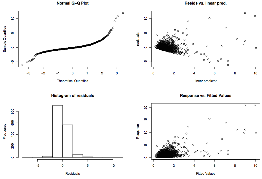
Example of "bad" plots
=======================
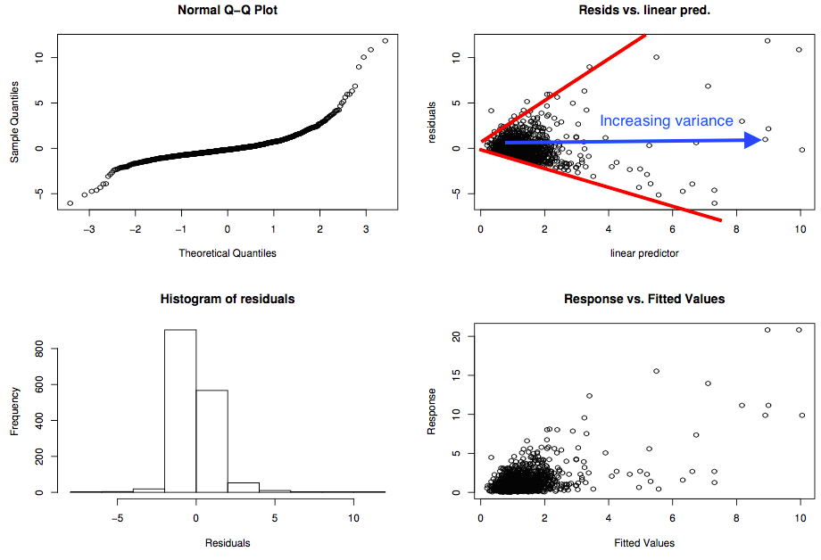
Residual checks
================
- Looking for patterns (not artifacts)
- This can be tricky
- Need to use a mixture of techniques
- Cycle through checks, make changes recheck
- Each dataset is different
Summary
=======
- Convergence
- Rarely an issue
- Check your thinking about the model
- Basis size
- k is a maximum
- Double and see what happens
- Residuals
- Deviance and randomised quantile
- check for artifacts
- `gam.check` is your friend