---
title: "BiSSE and HiSSE in R"
author: "Josh Justison"
date: "`r Sys.Date()`"
output:
html_document:
css: ../../Instructor_Materials/style/styles.css
knit: (function(inputFile, encoding) {
rmarkdown::render(inputFile, encoding = encoding, output_dir = "../") })
---
```{r setup, include=FALSE}
knitr::opts_chunk$set(echo = TRUE)
```
## Introduction
Plants have complex reproductive systems that can roughly be broken into two categories: self compatible (SC) plants that are hermaphrodidic and can self-fertilize and self incompatible (SI) where plants reject their own pollen for reproduction. Self compatibility has arisen multiple times across plants and both modes of reproduction are roughly equally abundant. It was hypothesized that SC plants may experience increased levels of inbreeding depression, and consequently, higher rates of extinction than their SI counterparts, making SI plants diversify more quickly than SC plants.
Interestingly, Goldberg and Igic ([2012](https://onlinelibrary.wiley.com/doi/full/10.1111/j.1558-5646.2012.01730.x)) used models of trait-dependent speciation and extinction to find that SI plants diversify at higher rates than SC plants.
These state-dependent speciation and extinction models, or $SSE$ type models are used to reflect the belief that rates of species diversification may depend on some trait that is itself changing over time.
Here we will be going over how to set up and use BiSSE and HiSSE models in R.
## Learning Objectives
* Be able to make and fit BiSSE models in R
+ Know how to constrain a BiSSE model
* Evaluate which models are a better fit, either through AIC or Log-likelihoods
* Comprehend the rate matrix of a HiSSE model and be able to make on in R
* Fit a HiSSE model given a phylogeny and data
## Scripts
For this lesson, we will be working with simulated data, so you will not need to download data files to execute these analayses. You can download the R script from the course repository:
* [`HiSSE_BiSSE_tutorial.R`](https://raw.githubusercontent.com/EEOB-Macroevolution/Practicals/main/BiSSE_HiSSE/scripts/HiSSE_BiSSE_tutorial.R)
* [`HiSSE_BiSSE_tutorial.Rmd`](https://raw.githubusercontent.com/EEOB-Macroevolution/Practicals/main/BiSSE_HiSSE/scripts/HiSSE_BiSSE_tutorial.Rmd)
## Background Material
This tutorial is based on the BiSSE and HiSSE tutorial by Luke Harmon: [https://lukejharmon.github.io/ilhabela/2015/07/05/BiSSE-and-HiSSE](https://lukejharmon.github.io/ilhabela/2015/07/05/BiSSE-and-HiSSE/).
For more background on the BiSSE and HiSSE models, please read:
* Harmon (2019), [Ch. 13 _Characters and diversification rates_](https://lukejharmon.github.io/pcm/chapter13_chardiv/)
* Maddison et al. (2007) [Estimating a Binary Character's Effect on Speciation and Extinction](https://academic.oup.com/sysbio/article/56/5/701/1694265)
* Beaulieu & O'Meara (2016) [Detecting Hidden Diversification Shifts in Models of Trait-Dependent Speciation and Extinction](https://academic.oup.com/sysbio/article/65/4/583/1753616?searchresult=1)
## Setup
The *BiSSE* model is implemented as part of the `diversitree` package, which also contains many other -SSE models, while the *HiSSE* model is implemented in the standalone package `hisse`. So we will start by installing and loading both of these packages.
```{r eval=FALSE}
install.packages("diversitree")
install.packages("hisse")
```
```{r}
##set the seed for reproducibility
set.seed(9177207) ##The exponent of the largest known repunit prime. ((10^9177207)-1)/9 is the prime
library(diversitree)
library(hisse)
```
## The BiSSE model
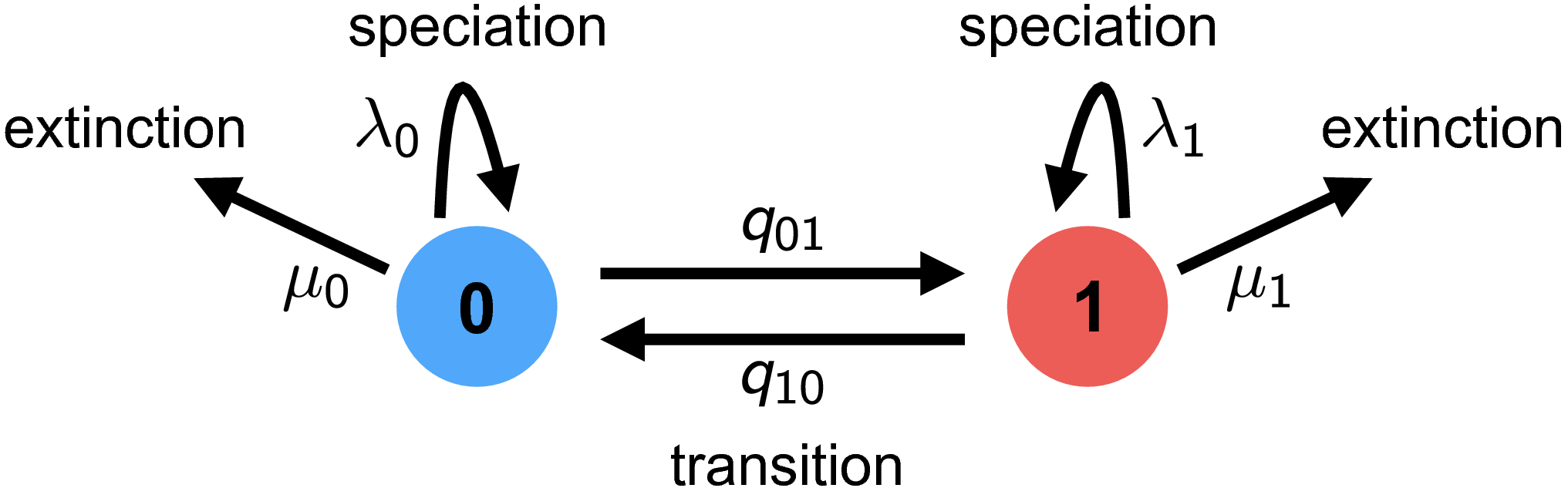
The Binary State-dependent Speciation and Extinction model is used when we believe that diversification rates depend on some binary character. This model has six parameters, $q_{01}$ and $q_{10}$ which describe the rate at which the binary character transitions from one state to another, and $\lambda_{0}$, $\mu_{0}$, $\lambda_{1}$, and $\mu_{1}$ which describe the diversification dynamics while a lineage is in state $0$ and $1$ respectively. Given a phylogeny and character values, we can estimate these parameters in R to learn about our system of interest.
### Setting up the BiSSE model in R
For our model we'll be using simulated phylogenetic and trait data. It's terribly important to understand how we simulated our data but for those interested, it is included in the box below.
**Simulating trees according to a BiSSE model**
We will be using the `tree.bisse()` function to simulate our data.
`tree.bisse()`
This function fits various models of continuous character evolution to trees. This function has many parameters but we'll be using the following ones:
This function takes a plethora of various arguments so it can be helpful to look at `?tree.bisse()` for documentation of these arguments. For our purposes we will be using the following arguments:
* $pars$: This is a vector containing all the associated parameters of the BiSSE model. Specifically, the vector has the parameters in this order $(\lambda_0,\lambda_1,\mu_1,\mu_0,q_{01},q_{10})$
* $max.taxa$: This is a number that specifies how many extant taxa we include in our simulation.
```{r}
sim_parameters <- c(1.0, 4, 0.7, 0.3, 0.2, 0.8)
names(sim_parameters)<-c('lambda0','lambda1','mu0','mu1','q01','q10')
tree_bisse <- tree.bisse(sim_parameters, max.taxa = 100)
tree_bisse
```
As you can see we have a phylogeny with 75 tips. As always with a phylogeny, we can use the `$` operator to look at the various components of our phylogeny. However, in the case of our simulation you can notice there are a few extra components related to the simulation and information about the trait evolution.
```{r}
names(tree_bisse) ##See which components exist for our simulated phylogeny.
```
Most notably, we can see a component called `tip.state`, this tells us which of the two states each tip is in. This is the type of data that researchers will have when trying to fit these types of models on a phylogeny.
```{r}
tree_bisse$tip.state
```
Some of these extra components from the simulation also give us historical information about which state past lineages were in. We can visualize the historical states with the code below. Here edges in state $0$ will be shown in red, and edges in state $1$ in blue while the colored dots on the right denote the state of extant lineages.
```{r}
treehistory = history.from.sim.discrete(tree_bisse, 0:1)
plot(treehistory, tree_bisse, cols = c("red", "blue"))
```
---
\
These data are simulated together under a BiSSE model where the diversification rates differ between the binary states. Specifically, we'll be assuming these parameters (used in `sim_parameters`):
```{r, echo=FALSE}
sim_parameters
```
We can see that $\lambda_1$ is higher than $\lambda_0$, meaning that lineages in state $1$ will speciate at a higher rate than those in state $0$. Knowing the conditions under which we simulate can be helpful for telling us both which models may be appropriate to use and whether our estimates were accurate.
### Fitting the BiSSE model
Now we will find out if BiSSE is able to correctly infer whether there are changes in the diversification rates on our simulated tree, by estimating the rates using maximum likelihood. We can use the `make.bisse()` function to create a $BiSSE$ model for our data.
`make.bisse()`
This simply attaches a BiSSE model to our simulated tree. This function has many different arguments but only two required ones that we'll be using:
* $tree$: This should be our phylogenetic tree. The tree should be bifurcating and ultrametric.
* $states$: This is a vector of tip states. The states in the vector should either be $0$ or $1$. The vector should have names that correspond to the tip labels in the phylogenetic tree (`tree$tip.label`). For example, in the simulated tree above we can see `names(tree_bisse$tip.state)` matches the names found in `tree_bisse$tip.label`. The order of the two vectors don't need to match exactly but they both should contain the same elements.
```{r}
bisse_model = make.bisse(tree_bisse, tree_bisse$tip.state)
```
Nice! We now have our $BiSSE$ model. The object returned is simply a likelihood function, it will give us the likelihood of our data (phylogeny and tip states) given some parameter values for $\lambda_0,\lambda_1,\mu_1,\mu_0,q_{01}, q_{10}$. We can actually see the assumptions this model and which parameters it needs just by typing out `bisse_model`. From there we can try inputting some parameter values to get a likelihood.
```{r}
bisse_model
```
From there we can try inputting some parameter values to get a likelihood. **Note:** the function returns a log-likelihood so we will be getting negative numbers, this avoids floating point error associated with representing small numbers on a computer.
```{r}
bisse_model(c(1.0, 4.0, 0.5, 0.5, 0.2, 0.8))
bisse_model(c(4.0, 1.0, 0 , 1 , 0.5, 0.5))
```
We can see that our first set of parameters returned a higher likelihood, this should be pretty reasonable as these are actually the parameters that simulated the model under! Our goal is to find the parameter values that maximize our likelihood function. We could try different combinations of values by hand but this would be very tedious and imprecise. Luckily, we have clever functions that attempt to maximize our likelihood.
Specifically, `find.mle()` can be used to find the maximum likelihood estimate (MLE) for our parameters.
`find.mle()`
This function has two main parameters:
* $lik$: This is our likelihood function for our model
* $x.init$: Initial values for our parameter estimates.
We can try finding the parameters that maximize our likelihood as long as we have some initial values. We can use `starting.point.bisse()` to get reasonable starting values.
```{r}
initial_pars<-starting.point.bisse(tree_bisse)
fit_model<-find.mle(bisse_model,initial_pars)
```
**Note:** Contrary to the name of the function, `find.mle()` doesn't guarantee that we actually find the parameters that maximize the likelihood as `find.mle()` is a [greedy algorithm](https://en.wikipedia.org/wiki/Greedy_algorithm), meaning that it will find a local optimum which may or may not be the global optimum that maximizes likelihood. As a result, we may get a different results based on the initial values we choose. It can be a good practice to try a few different starting points with `find.mle()` and if they converge on the same set of parameter values then we can be more confident that we are at a global optimum.
The object returned from `find.mle()` has a slew of different components. Two componenets that might be useful for us are the log-likelihood of the fit model and the parameter estimates, these are denoted with `lnLik` and `par` respectively.
```{r}
fit_model$lnLik
round(fit_model$par,digits=2) ##we round to two digits for easier reading
```
We can now compare our fit model to the true parameters that we used for simulation.
```{r}
sim_parameters
```
Although, we don't get the same estimates as the simulation condition, it seems that our fit model captures the idea that the two states have different speciation parameters. However, our fit model also estimated different extinction parameters for each state when in fact we simulated with both states having $\mu=0.5$. As such, we may wish to create a model where the $\mu's$ are constrained to be the same.
We can use the `constrain()` function to constrain certain parameters of our model.
`constrain()`
This function has two main arguments:
* $f$: This is the likelihood function or model that will be getting additional constraints
* $formulae$: This is where we add formulae that constrain our parameters.
Constraint formulae typically take the format `x ~ y`. This can be interpreted as '`x` is constrained to the value of `y`', meaning that parameter `x` will take on the same values as `y`. `y` can be a constant value (e.g. `mu1~3`), a parameter from the model (e.g. `lambda0 ~ lambda1`), or some expression of parameters (e.g. `lambda0 ~ (2*lambda1)-mu1`). When it comes to setting the values of extinction to be the same between states, we just need to constrain one of the $\mu's$ to the other $\mu$.
```{r}
constrained_bisse_model <-constrain(bisse_model,mu0 ~ mu1)
```
In our case we constrained `mu0` to be the same as `mu1`. We can now use `find.mle` as we did before to fit our model, the only difference is that we will remove a starting value for `mu0` since `mu0` is constrained to be the same as `mu1`.
```{r}
constrained_initial_pars<-initial_pars[-3]
fit_constrained_model <- find.mle(constrained_bisse_model,constrained_initial_pars)
round(fit_constrained_model$par,digits = 2) ##Round estimates to 2 digits for simplicity
```
We can compare the fit of our unconstrained and constrained models with the `anova()` function. We simply need to enter the two fit models into the function.
```{r}
anova(fit_model,constrained=fit_constrained_model)
```
The AIC comparison of the two models shows that the constrained model is a better fit for our simulated data, although since AIC scores are so close we probably can't distinguish between the two models.
## Detecting changes in diversification rates with HiSSE
One issue with the BiSSE model is that it has trouble distinguishing between changes in rates that are tied to the character state tested, and changes in rates which are independent of that character.
The HiSSE model (hidden-state dependent speciation and extinction) incorporates a 2nd, unobserved character to account for correlations that are not tied to the character we are testing.
Changes in the unobserved character’s state represent background diversification rate shifts that are uncorrelated with the observed character [[Beaulieu & O'Meara 2016](https://doi.org/10.1093/sysbio/syw022)].
Let's start by simulating a secondary character for our tree.
```{r}
##simulate binary trait data on the tree
transition_rates<-c(0.5,1)
secondary_trait <- sim.character(tree = tree_bisse, pars =transition_rates , x0 = 1, model='mk2')
```
Since we simulated binary character data after the tree was already generated, the traits we simulated are independent of the diversification dynamics. In other words, we should not find that the two states have different diversification rate estimates.
We can then we run ML estimation using the BiSSE model and this new character.
```{r}
incorrect_bisse_model <- make.bisse(tree_bisse, secondary_trait)
incorrect_bisse_mle <- find.mle(incorrect_bisse_model, initial_pars)
```
We will also try a null model where both birth rates and death rates are identical between states. This model should more accurately reflect our simulation conditions as these secondary states shouldn't have different diversification dynamics.
```{r}
incorrect_null_bisse_model <- constrain(incorrect_bisse_model, lambda0 ~ lambda1)
incorrect_null_bisse_model <- constrain(incorrect_null_bisse_model, mu0 ~ mu1)
constrained_initial_pars<-initial_pars[c(-1,-3)]
incorrect_null_bisse_mle <- find.mle(incorrect_null_bisse_model, constrained_initial_pars)
```
Finally, we can again compare the fit of both models
```{r}
anova(incorrect_bisse_mle, constrained = incorrect_null_bisse_mle)
```
Here we see that the constrained has a lower AIC score than the unconstrained model. Although it should be noted that both models do a poor job at describing the true conditions as there are trait dependent diversification dynamics, it just so happens that those dynamics are the result of the first trait we used and not this secondary one.
The HiSSE model was developed to address this issue, by implementing a better null model than the simple constrained one we have been using so far. Note that the `hisse` package was developed independently from `diversitree`, so its syntax is going to be quite different.
We want to test whether the changes in rates are due to the observed character or to a hidden one, so first we will build a null model where the rates only depend on a hidden character. In our case we actually know and have access to the character that actually causes a change in rates, but for the purposes of demonstration, we will pretend that we don't have that information and only have trait data for our secondary character.
We can create and run our model with the `hisse()` function.
`hisse()`
We will be using the following arguments for this function:
* $phy$:This is our phylogenetic tree.
* $data$ This is a dataframe with our trait information. The dataframe has two columns: the first column has the species names while the second column has the character states for each species
* $turnover$: This is a vector that denotes which states will have identical turnover rates.
* $eps$: This is a vector that denotes which states will have identical extinction fraction rates.
* $hidden.states$: a logical TRUE/FALSE that indicates whether the model has hidden states.
* $trans.rate$: provides the model for the rate that species transition from one state to another.
There are quite a few arguements and some of them may be unfamiliar. We will go over how to interpret and set up the `trans.rate`, `turnover`, and `eps` arguments below.
The first step is to build a transition rate matrix for the null model. To do this we will use `TransMatMakerHiSSE()`.
`TransMatMakerHiSSE()`
We will be using the following arguments for this function:
We will be using two arguments for this function:
* $hidden.traits$: This is a numeric value that specifies how many hidden states are in the model. If we set `hidden.traits=0` then this would be the same as the BiSSE model.
* $make.null$: This argument takes a logical TRUE/FALSE and sets the matrix to be the null model where (1) transition rates are the same across all hidden states and (2) the transition rates between hidden states are the same.
```{r}
null_rate_matrix <- TransMatMakerHiSSE(hidden.traits = 1,make.null=T)
null_rate_matrix
```
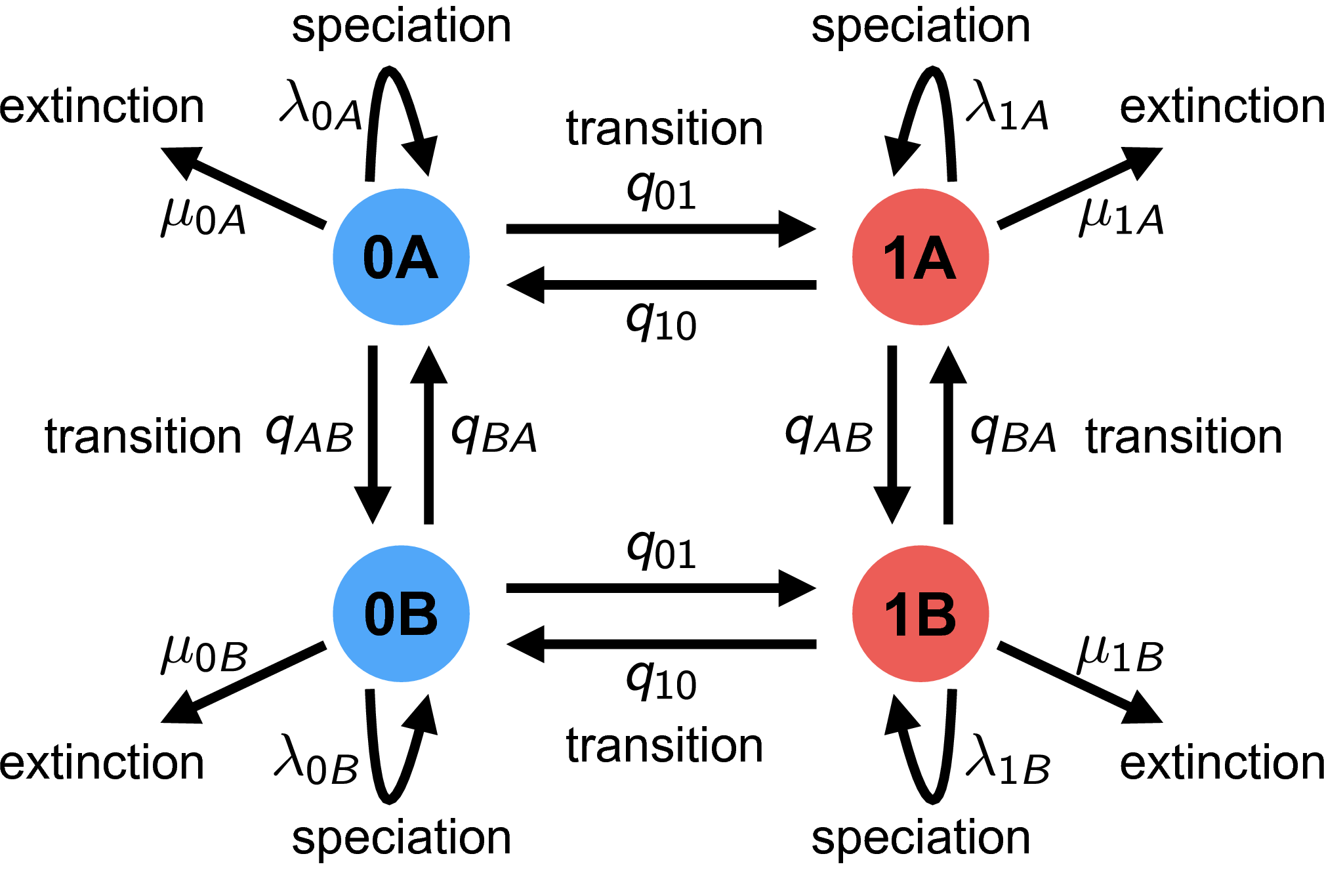
The observed characters are denoted with either a $0$ or a $1$ while the hidden characters are denoted with $A$ and $B$
The markings of 1, 2, or 3 don't tell us what the actual rates are, just that elements with the same number will share a rate in our model. This is similar to the `constrain()` function we used in the BiSSE model but instead we are constraining certain transition rates to be equal.
We can see that whenever there is a transition from $A \leftrightarrow{B}$ they all have the same rate (denoted with 1), regardless of whether we're in state $1$ or $2$. We can also see transitions from $1\rightarrow{0}$ all have the same rate and are denoted with a 1 while transitions from $0\rightarrow{1}$ have the same rate denoted by all having a 2. We can also see a few `NA`s in our matrix, we see these whenever we see both states transition at once ( $1A \leftrightarrow{0B}$ or $0A \leftrightarrow{1B}$). Generally, we assume that only one state changes at a given time so we want to exclude the possibility that both transitions occur at once.
Next we need to specify which diversification rates are shared between states. Unlike `diversitree`, `hisse` has uses a different parameterization for diversification. Instead of speciation and extinction, `hisse` uses net turnover and the extinction fraction. While these sound odd, don't be alarmed as they are just transformations of speciation and extinction. Specifically they are:
* $net\ turnover= \lambda+\mu$
* $extinction\ fraction = \mu/\lambda$
The states are ordered 0A, 1A, 0B, 1B, so we will specify that the diversification rates are identical between 0 and 1 but can differ between A and B - i.e. that states 0A and 1A share one value, and 0B and 1B share another. We chose to specify these values to model the idea that changes in diversification are solely due to the hidden state and not the trait data we provide.
```{r}
null_net_turnover <- c(1,1,2,2)
null_extinction_fraction <- c(1,1,2,2)
```
And finally we will transform the tip character we simulated previously into the HiSSE format.
```{r}
hisse_states <- cbind(names(secondary_trait), secondary_trait)
```
Now we can run the ML estimation on the *HiSSE* null model.
```{r}
null_hisse <- hisse(phy = tree_bisse, data = hisse_states, hidden.states=TRUE,
turnover = null_net_turnover, eps = null_extinction_fraction,
trans.rate = null_rate_matrix)
null_hisse
```
We can now compare our `null_hisse` model to our previous `incorrect_bisse` and `null_incorrect_bisse models`.
```{r}
null_hisse$AIC
AIC(incorrect_bisse_mle)
AIC(incorrect_null_bisse_mle)
```
We can see that our `null_hisse` model has the lowest AIC, we might interpret this as some other trait than our secondary trait controlling the change in diversification rates, and it should, the first trait we simulated is the one that has differential speciation rates!
We can also set up a $HiSSE$ model with our first trait. In this case we would hope that the $HiSSE$ model actually performs worse since we will be using the trait that actually changes diversfication rates.
```{r}
hisse_states2 <- cbind(names(tree_bisse$tip.state), tree_bisse$tip.state)
null_hisse2 <- hisse(phy = tree_bisse, data = hisse_states2, hidden.states=TRUE,
turnover = null_net_turnover, eps = null_extinction_fraction,
trans.rate = null_rate_matrix)
```
And again we can compare the AIC values obtained.
```{r}
null_hisse2$AIC
AIC(fit_model)
AIC(fit_constrained_model)
```
Here we can see the null $HiSSE$ model actually was a poor fit and AIC value for the `constrained_bisse_mle` model indicates that the data fit this model the best.
## Try it out - Tribble Diversification
Here we will be looking at the diversification of the fictional species of [Tribbles](https://en.wikipedia.org/wiki/Tribble) from the Startrek universe. Tribbles are little balls of fur that reproduce at a prolific rate. [Klingons are the natural predators](https://www.youtube.com/watch?v=1FTNPtANZXQ) of the Tribbles. As a defense mechanism, some species of Tribble have developed the ability to squeal when in the presence of a Klingon. The ability to squeal has led some scientists to hypothesize that the release from predation has led to an increase in net diversification ($\lambda-\mu$). We can use the BiSSE and HiSSE models to evaluate this hypothesis
### Step 1: Read in the data
First, you will want to read in the `Tribble_ml.tre` file for the Tribble phylogeny and `Tribble_trait_data.csv` for the data on Squealing Tribbles. In the csv we denote $1$ as a Tribble that does squeal when among Klingons and a $0$ is a Tribble that does not squeal.
*Note*: `Tribble_trait_data.csv` is in the format we would want for a $HiSSE$ model but we will need to put this data in a named vector for the $BiSSE$ model, you may want to do this now.
### Step 2: Run up $BiSSE$ models
Now you will want to set up two $BiSSE$ models, one where $\lambda$ and $\mu$ are allowed to vary between states and another model where $\lambda$ and $\mu$ are constrained to be the same between states. You will need to find the best fit of these models.
What is the net diversification of the two states ($\lambda-\mu$) between the two models? Which model was a better fit? What does this mean for the diversification of Tribbles, do you think the squealing has led to higher net diversification?
### Step 3: Set up and run $HiSSE$ model
Here you will want to set up a null $HiSSE$ model that assesses whether some other hidden trait may be controlling the change in diversification. Compare this model to the $BiSSE$ models above, does it seem like some other trait does a better job at determining changes in diversification rates? Does this change your interpretation from above? Which results are more trustworthy and why?
### Step 4 Uncertainty in the Tribble phylogeny
If we did a Bayesian analysis on the Tribble phylogeny we would get a posterior set of trees that represent the uncertainty in the Tribble phylogeny. We may wish to run these models on our posterior set of trees to get an idea for how robust our results are to phylogenetic uncertainty. In the `data` folder read in the posterior set of trees found in `tribble_bayesian.tre`.
Here you will find 50 different trees from our posterior. Try running the $BiSSE$ and $HiSSE$ models on the posterior set of trees, recording the model that has the best fit (has the lowest AIC) and the net diversification for each state. *Note* Since the $HiSSE$ model uses a reparameterization of the speciation and extinction rate you will need to do a bit of algebra to compute net diversification if it is the best fit.
Which model tended to fit the best? What was the average net diversification among the two states for the best fit model? Make two histograms with the net diversification of the best fit models of the posterior trees, Does it look like they differ?