 ```python
#!/usr/bin/env python3
import random
import os
import sys
BOARD_SIZE = 4
TARGET = 2048
def init_board():
board = [[0] * BOARD_SIZE for _ in range(BOARD_SIZE)]
add_random_tile(board)
add_random_tile(board)
return board
def add_random_tile(board):
empty = [(i, j) for i in range(BOARD_SIZE) for j in range(BOARD_SIZE) if board[i][j] == 0]
if not empty:
return
i, j = random.choice(empty)
board[i][j] = 4 if random.random() < 0.1 else 2
def print_board(board):
os.system('clear') # 清屏
print("-" * (BOARD_SIZE * 7 + 1))
for row in board:
print("|", end="")
for num in row:
if num == 0:
print(" |", end="")
else:
print(f"{num:^6}|", end="")
print()
print("-" * (BOARD_SIZE * 7 + 1))
def slide_and_merge(line):
new_line = [num for num in line if num != 0]
merged_line = []
skip = False
for i in range(len(new_line)):
if skip:
skip = False
continue
if i + 1 < len(new_line) and new_line[i] == new_line[i + 1]:
merged_line.append(new_line[i] * 2)
skip = True
else:
merged_line.append(new_line[i])
merged_line += [0] * (BOARD_SIZE - len(merged_line))
return merged_line
def move_left(board):
return [slide_and_merge(row) for row in board]
def reverse(board):
return [list(reversed(row)) for row in board]
def transpose(board):
return [list(row) for row in zip(*board)]
def move_right(board):
return reverse(move_left(reverse(board)))
def move_up(board):
transposed = transpose(board)
moved = move_left(transposed)
return transpose(moved)
def move_down(board):
transposed = transpose(board)
moved = move_right(transposed)
return transpose(moved)
def boards_equal(b1, b2):
for i in range(BOARD_SIZE):
for j in range(BOARD_SIZE):
if b1[i][j] != b2[i][j]:
return False
return True
def can_move(board):
for row in board:
if 0 in row:
return True
for i in range(BOARD_SIZE):
for j in range(BOARD_SIZE):
if j + 1 < BOARD_SIZE and board[i][j] == board[i][j + 1]:
return True
if i + 1 < BOARD_SIZE and board[i][j] == board[i + 1][j]:
return True
return False
def reached_target(board):
for row in board:
if any(num >= TARGET for num in row):
return True
return False
def main():
board = init_board()
has_printed_win = False # 避免重复打印获胜消息
print_board(board)
while True:
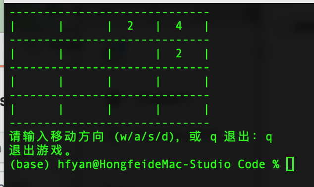
move = input("请输入移动方向 (w/a/s/d),或 q 退出:").lower().strip()
if move not in ['w', 'a', 's', 'd', 'q']:
continue
if move == 'q':
print("退出游戏。")
sys.exit(0)
if move == 'w':
new_board = move_up(board)
elif move == 'a':
new_board = move_left(board)
elif move == 's':
new_board = move_down(board)
elif move == 'd':
new_board = move_right(board)
if not boards_equal(board, new_board):
board = new_board
add_random_tile(board)
else:
print("无效移动!")
print_board(board)
if reached_target(board) and not has_printed_win:
print("恭喜你达到了 2048!当然,如果能合成更大的数字就更好!")
has_printed_win = True
if not can_move(board):
print("游戏结束,无法移动!")
break
if __name__ == "__main__":
main()
```
**使用说明**
1. 将代码保存为文件(例如 `game_2048.py`)。
2. 在终端中执行 `chmod +x game_2048.py` 给予执行权限。
3. 运行 `./game_2048.py` 启动游戏。
游戏中输入 `w/a/s/d` 分别控制上、左、下、右移动,输入 `q` 退出。达到 2048 后会显示提示,但你仍可继续游戏,挑战更高的分数。
### 2. auto_2048.py
帮我做一个升级版本,就是自动演示上下左右移动的2048游戏
下面是一份自动演示版 2048 游戏的 Python 代码,运行时会自动随机选择上、下、左、右移动,并在终端中展示移动过程。你可以直接在 Mac Terminal 中运行该脚本:
```python
#!/usr/bin/env python3
import random
import os
import sys
import time
BOARD_SIZE = 4
TARGET = 2048
def init_board():
board = [[0] * BOARD_SIZE for _ in range(BOARD_SIZE)]
add_random_tile(board)
add_random_tile(board)
return board
def add_random_tile(board):
empty = [(i, j) for i in range(BOARD_SIZE) for j in range(BOARD_SIZE) if board[i][j] == 0]
if not empty:
return
i, j = random.choice(empty)
# 以 10% 的概率生成 4,其余生成 2
board[i][j] = 4 if random.random() < 0.1 else 2
def print_board(board):
os.system('clear') # 清屏
print("-" * (BOARD_SIZE * 7 + 1))
for row in board:
print("|", end="")
for num in row:
if num == 0:
print(" |", end="")
else:
print(f"{num:^6}|", end="")
print()
print("-" * (BOARD_SIZE * 7 + 1))
def slide_and_merge(line):
# 去除所有零值
new_line = [num for num in line if num != 0]
merged_line = []
skip = False
for i in range(len(new_line)):
if skip:
skip = False
continue
# 若相邻数字相等,则合并
if i + 1 < len(new_line) and new_line[i] == new_line[i + 1]:
merged_line.append(new_line[i] * 2)
skip = True
else:
merged_line.append(new_line[i])
# 补0使长度固定
merged_line += [0] * (BOARD_SIZE - len(merged_line))
return merged_line
def move_left(board):
new_board = []
for row in board:
new_board.append(slide_and_merge(row))
return new_board
def reverse(board):
return [list(reversed(row)) for row in board]
def transpose(board):
return [list(row) for row in zip(*board)]
def move_right(board):
return reverse(move_left(reverse(board)))
def move_up(board):
transposed = transpose(board)
moved = move_left(transposed)
return transpose(moved)
def move_down(board):
transposed = transpose(board)
moved = move_right(transposed)
return transpose(moved)
def boards_equal(b1, b2):
for i in range(BOARD_SIZE):
for j in range(BOARD_SIZE):
if b1[i][j] != b2[i][j]:
return False
return True
def can_move(board):
# 若有空格则肯定能移动
for row in board:
if 0 in row:
return True
# 检查水平和垂直是否有可合并的数字
for i in range(BOARD_SIZE):
for j in range(BOARD_SIZE):
if j + 1 < BOARD_SIZE and board[i][j] == board[i][j + 1]:
return True
if i + 1 < BOARD_SIZE and board[i][j] == board[i + 1][j]:
return True
return False
def reached_target(board):
for row in board:
if any(num >= TARGET for num in row):
return True
return False
def main():
board = init_board()
has_printed_win = False # 避免重复打印获胜消息
print_board(board)
while True:
if not can_move(board):
print("游戏结束,无法移动!")
break
# 自动随机选择一个方向
move = random.choice(['w', 'a', 's', 'd'])
print(f"自动移动:{move}")
if move == 'w':
new_board = move_up(board)
elif move == 'a':
new_board = move_left(board)
elif move == 's':
new_board = move_down(board)
elif move == 'd':
new_board = move_right(board)
if not boards_equal(board, new_board):
board = new_board
add_random_tile(board)
else:
print("无效移动,尝试其他方向。")
print_board(board)
if reached_target(board) and not has_printed_win:
print("已达到 2048!继续自动移动以获得更高分数。")
has_printed_win = True
time.sleep(0.01) # 延时0.5秒,便于观察演示效果
if __name__ == "__main__":
main()
```
---
**使用说明**
1. 将上述代码保存为文件(例如 `auto_2048.py`)。
2. 在终端中运行命令 `chmod +x auto_2048.py` 赋予执行权限。
3. 运行 `./auto_2048.py` 启动自动演示。
程序将自动随机选择上、下、左、右方向进行移动,并以 0.5 秒的间隔更新显示。你可以通过修改 `time.sleep` 的延时参数来调整演示速度。
### 3. auto_2048_intelligent.py
能智能些吗?刚运行auto_2048,才累积到128,就游戏结束无法移动了。
下面是一份升级版自动演示 2048 游戏代码,加入了简单的启发式策略。程序会对四个方向的移动进行模拟,选择能使空格最多的那一步,从而尽量延长游戏时间,避免早期卡死。你可以直接在 Mac Terminal 下运行该脚本:
```python
#!/usr/bin/env python3
import random
import os
import sys
import time
BOARD_SIZE = 4
TARGET = 2048
def init_board():
board = [[0] * BOARD_SIZE for _ in range(BOARD_SIZE)]
add_random_tile(board)
add_random_tile(board)
return board
def add_random_tile(board):
empty = [(i, j) for i in range(BOARD_SIZE) for j in range(BOARD_SIZE) if board[i][j] == 0]
if not empty:
return
i, j = random.choice(empty)
board[i][j] = 4 if random.random() < 0.1 else 2
def print_board(board):
os.system('clear') # 清屏
print("-" * (BOARD_SIZE * 7 + 1))
for row in board:
print("|", end="")
for num in row:
if num == 0:
print(" |", end="")
else:
print(f"{num:^6}|", end="")
print()
print("-" * (BOARD_SIZE * 7 + 1))
def slide_and_merge(line):
new_line = [num for num in line if num != 0]
merged_line = []
skip = False
for i in range(len(new_line)):
if skip:
skip = False
continue
if i + 1 < len(new_line) and new_line[i] == new_line[i + 1]:
merged_line.append(new_line[i] * 2)
skip = True
else:
merged_line.append(new_line[i])
merged_line += [0] * (BOARD_SIZE - len(merged_line))
return merged_line
def move_left(board):
return [slide_and_merge(row) for row in board]
def reverse(board):
return [list(reversed(row)) for row in board]
def transpose(board):
return [list(row) for row in zip(*board)]
def move_right(board):
return reverse(move_left(reverse(board)))
def move_up(board):
transposed = transpose(board)
moved = move_left(transposed)
return transpose(moved)
def move_down(board):
transposed = transpose(board)
moved = move_right(transposed)
return transpose(moved)
def boards_equal(b1, b2):
for i in range(BOARD_SIZE):
for j in range(BOARD_SIZE):
if b1[i][j] != b2[i][j]:
return False
return True
def can_move(board):
for row in board:
if 0 in row:
return True
for i in range(BOARD_SIZE):
for j in range(BOARD_SIZE):
if j + 1 < BOARD_SIZE and board[i][j] == board[i][j + 1]:
return True
if i + 1 < BOARD_SIZE and board[i][j] == board[i + 1][j]:
return True
return False
def reached_target(board):
for row in board:
if any(num >= TARGET for num in row):
return True
return False
def count_empty(board):
return sum(row.count(0) for row in board)
def choose_best_move(board):
moves = {
'w': move_up,
'a': move_left,
's': move_down,
'd': move_right
}
best_move = None
best_score = -1
best_new_board = None
for move, func in moves.items():
new_board = func(board)
if boards_equal(board, new_board):
continue
score = count_empty(new_board)
if score > best_score:
best_score = score
best_move = move
best_new_board = new_board
return best_move, best_new_board
def main():
board = init_board()
has_printed_win = False
print_board(board)
while True:
if not can_move(board):
print("游戏结束,无法移动!")
break
move, new_board = choose_best_move(board)
if move is None:
print("没有有效移动,游戏结束!")
break
print(f"自动移动:{move}")
board = new_board
add_random_tile(board)
print_board(board)
if reached_target(board) and not has_printed_win:
print("已达到 2048!继续自动移动以获得更高分数。")
has_printed_win = True
time.sleep(0.01)
if __name__ == "__main__":
main()
```
---
使用说明
1. 将上述代码保存为文件(例如 `auto_2048_intelligent.py`)。
2. 在终端中执行 `chmod +x auto_2048_intelligent.py` 赋予执行权限。
3. 运行 `./auto_2048_intelligent.py` 启动自动演示。
程序会自动选择四个方向中使空格最多的移动方向,尽量保持棋盘宽松,帮助你累积到更高的分数。你也可以调整 `time.sleep` 延时参数来观察移动过程。
### 4. auto_2048_ai.py
还是不够智能,到128就结束了
下面是一份升级版自动演示 2048 游戏代码,采用了简单的“1 层期望搜索(expectimax)”策略和启发式评估函数,从而尽可能选择对局面更有利的移动。该代码在模拟每个可能移动后,对随机新增块进行平均评估,然后选择评分最高的移动方向,从而延长游戏时间,争取更高分数:
```python
#!/usr/bin/env python3
import random
import os
import sys
import time
import copy
BOARD_SIZE = 4
TARGET = 2048
def init_board():
board = [[0] * BOARD_SIZE for _ in range(BOARD_SIZE)]
add_random_tile(board)
add_random_tile(board)
return board
def add_random_tile(board):
empty = [(i, j) for i in range(BOARD_SIZE) for j in range(BOARD_SIZE) if board[i][j] == 0]
if not empty:
return
i, j = random.choice(empty)
board[i][j] = 4 if random.random() < 0.1 else 2
def print_board(board):
os.system('clear') # Mac/Linux 下清屏
print("-" * (BOARD_SIZE * 7 + 1))
for row in board:
print("|", end="")
for num in row:
if num == 0:
print(" |", end="")
else:
print(f"{num:^6}|", end="")
print()
print("-" * (BOARD_SIZE * 7 + 1))
def slide_and_merge(line):
# 去除0值
new_line = [num for num in line if num != 0]
merged_line = []
skip = False
for i in range(len(new_line)):
if skip:
skip = False
continue
if i + 1 < len(new_line) and new_line[i] == new_line[i+1]:
merged_line.append(new_line[i] * 2)
skip = True
else:
merged_line.append(new_line[i])
merged_line += [0] * (BOARD_SIZE - len(merged_line))
return merged_line
def move_left(board):
return [slide_and_merge(row) for row in board]
def reverse(board):
return [list(reversed(row)) for row in board]
def transpose(board):
return [list(row) for row in zip(*board)]
def move_right(board):
return reverse(move_left(reverse(board)))
def move_up(board):
transposed = transpose(board)
moved = move_left(transposed)
return transpose(moved)
def move_down(board):
transposed = transpose(board)
moved = move_right(transposed)
return transpose(moved)
def boards_equal(b1, b2):
for i in range(BOARD_SIZE):
for j in range(BOARD_SIZE):
if b1[i][j] != b2[i][j]:
return False
return True
def can_move(board):
for row in board:
if 0 in row:
return True
for i in range(BOARD_SIZE):
for j in range(BOARD_SIZE):
if j+1 < BOARD_SIZE and board[i][j] == board[i][j+1]:
return True
if i+1 < BOARD_SIZE and board[i][j] == board[i+1][j]:
return True
return False
def reached_target(board):
for row in board:
if any(num >= TARGET for num in row):
return True
return False
def count_empty(board):
return sum(row.count(0) for row in board)
def evaluate_board(board):
"""
一个简单的评估函数,综合考虑:
1. 空格数:空格越多越好(乘以较大权重)
2. 最大数字是否在角落:在角落奖励
3. 行列单调性:如果整行或整列是单调的,给予一定奖励
"""
score = count_empty(board) * 100
max_tile = max(max(row) for row in board)
# 如果最大数字在角落,则奖励
corners = [board[0][0], board[0][BOARD_SIZE-1], board[BOARD_SIZE-1][0], board[BOARD_SIZE-1][BOARD_SIZE-1]]
if max_tile in corners:
score += max_tile * 10
# 行单调性奖励
for row in board:
if all(row[i] >= row[i+1] for i in range(len(row)-1)) or all(row[i] <= row[i+1] for i in range(len(row)-1)):
score += sum(row) * 0.1
# 列单调性奖励
for col in zip(*board):
if all(col[i] >= col[i+1] for i in range(len(col)-1)) or all(col[i] <= col[i+1] for i in range(len(col)-1)):
score += sum(col) * 0.1
return score
def expectimax_value(board):
"""
1层期望搜索:
对当前局面,模拟在每个空格上随机生成2(概率0.9)或4(概率0.1),
返回平均评估得分。
"""
empty = [(i, j) for i in range(BOARD_SIZE) for j in range(BOARD_SIZE) if board[i][j] == 0]
if not empty:
return evaluate_board(board)
total = 0
for (i, j) in empty:
board2 = copy.deepcopy(board)
board2[i][j] = 2
score2 = evaluate_board(board2)
board4 = copy.deepcopy(board)
board4[i][j] = 4
score4 = evaluate_board(board4)
total += 0.9 * score2 + 0.1 * score4
return total / len(empty)
def choose_best_move(board):
moves = {
'w': move_up,
'a': move_left,
's': move_down,
'd': move_right
}
best_move = None
best_score = -float('inf')
best_new_board = None
for move, func in moves.items():
new_board = func(board)
if boards_equal(board, new_board):
continue
# 使用1层期望搜索的评估
score = expectimax_value(new_board)
if score > best_score:
best_score = score
best_move = move
best_new_board = new_board
return best_move, best_new_board
def main():
board = init_board()
has_printed_win = False
print_board(board)
while True:
if not can_move(board):
print("游戏结束,无法移动!")
break
move, new_board = choose_best_move(board)
if move is None:
print("没有有效移动,游戏结束!")
break
print(f"自动移动:{move}")
board = new_board
add_random_tile(board)
print_board(board)
if reached_target(board) and not has_printed_win:
print("已达到 2048!继续自动移动以获得更高分数。")
has_printed_win = True
time.sleep(0.01)
if __name__ == "__main__":
main()
```
---
**使用说明**
1. 将上述代码保存为文件(例如 `auto_2048_ai.py`)。
2. 在终端中执行 `chmod +x auto_2048_ai.py` 赋予执行权限。
3. 运行 `./auto_2048_ai.py` 启动自动演示。
此版本采用了简单的启发式评估和1层期望搜索:
• 每个可能的移动后,程序会模拟在所有空位上新增数字(2 和 4)后计算平均评估分数;
• 评估函数综合考虑了空格数量、最大数字是否处于角落以及行列的单调性。
这样有助于程序选择更加“智能”的移动方向,争取获得更高的分数而不是早早卡死。
请根据需要调整权重和延时(time.sleep)参数以获得最佳效果。
### 5.auto_2048_expectimax.py
还是不够智能,到256就结束了
下面这份代码使用了多层(深度 3)期望搜索(expectimax),并在评估函数中加入了角落权重、空格奖励以及行列单调性奖励,以期使 AI 在选择移动时更“聪明”,尽量避免早期卡死。请注意,由于搜索深度增加,运行速度可能会变慢一些,但通常能在 4×4 棋盘上接受。
```python
#!/usr/bin/env python3
import random
import os
import sys
import time
import copy
BOARD_SIZE = 4
TARGET = 2048
SEARCH_DEPTH = 3 # 增加搜索深度
def init_board():
board = [[0] * BOARD_SIZE for _ in range(BOARD_SIZE)]
add_random_tile(board)
add_random_tile(board)
return board
def add_random_tile(board):
empty = [(i, j) for i in range(BOARD_SIZE) for j in range(BOARD_SIZE) if board[i][j] == 0]
if not empty:
return
i, j = random.choice(empty)
board[i][j] = 4 if random.random() < 0.1 else 2
def print_board(board):
os.system('clear') # Mac/Linux 下清屏
print("-" * (BOARD_SIZE * 7 + 1))
for row in board:
print("|", end="")
for num in row:
if num == 0:
print(" |", end="")
else:
print(f"{num:^6}|", end="")
print()
print("-" * (BOARD_SIZE * 7 + 1))
def slide_and_merge(line):
new_line = [num for num in line if num != 0]
merged_line = []
skip = False
for i in range(len(new_line)):
if skip:
skip = False
continue
if i + 1 < len(new_line) and new_line[i] == new_line[i + 1]:
merged_line.append(new_line[i] * 2)
skip = True
else:
merged_line.append(new_line[i])
merged_line += [0] * (BOARD_SIZE - len(merged_line))
return merged_line
def move_left(board):
return [slide_and_merge(row) for row in board]
def reverse(board):
return [list(reversed(row)) for row in board]
def transpose(board):
return [list(row) for row in zip(*board)]
def move_right(board):
return reverse(move_left(reverse(board)))
def move_up(board):
return transpose(move_left(transpose(board)))
def move_down(board):
return transpose(move_right(transpose(board)))
def boards_equal(b1, b2):
for i in range(BOARD_SIZE):
for j in range(BOARD_SIZE):
if b1[i][j] != b2[i][j]:
return False
return True
def can_move(board):
for row in board:
if 0 in row:
return True
for i in range(BOARD_SIZE):
for j in range(BOARD_SIZE):
if j + 1 < BOARD_SIZE and board[i][j] == board[i][j + 1]:
return True
if i + 1 < BOARD_SIZE and board[i][j] == board[i + 1][j]:
return True
return False
def reached_target(board):
for row in board:
if any(num >= TARGET for num in row):
return True
return False
def evaluate_board(board):
score = 0
# 奖励空格
empty = sum(row.count(0) for row in board)
score += empty * 100
# 使用一个预设的权重矩阵,鼓励最大值位于角落(这里采用蛇形布局)
weights = [
[65536, 32768, 16384, 8192],
[512, 1024, 2048, 4096],
[256, 512, 1024, 2048],
[128, 256, 512, 1024]
]
for i in range(BOARD_SIZE):
for j in range(BOARD_SIZE):
score += board[i][j] * weights[i][j]
# 奖励行单调性
for row in board:
if all(row[i] >= row[i+1] for i in range(len(row)-1)) or all(row[i] <= row[i+1] for i in range(len(row)-1)):
score += sum(row)
# 奖励列单调性
for col in zip(*board):
if all(col[i] >= col[i+1] for i in range(len(col)-1)) or all(col[i] <= col[i+1] for i in range(len(col)-1)):
score += sum(col)
return score
def expectimax(board, depth, is_player):
if depth == 0 or not can_move(board):
return evaluate_board(board)
if is_player:
best = -float('inf')
# 玩家节点:尝试所有四个方向
for move_func in [move_up, move_down, move_left, move_right]:
new_board = move_func(board)
if boards_equal(board, new_board):
continue
value = expectimax(new_board, depth, False)
best = max(best, value)
return best if best != -float('inf') else evaluate_board(board)
else:
# 概率节点:模拟在所有空格上随机出现 2 或 4
empty = [(i, j) for i in range(BOARD_SIZE) for j in range(BOARD_SIZE) if board[i][j] == 0]
if not empty:
return evaluate_board(board)
total = 0.0
for (i, j) in empty:
for tile, prob in [(2, 0.9), (4, 0.1)]:
new_board = copy.deepcopy(board)
new_board[i][j] = tile
total += prob * expectimax(new_board, depth - 1, True)
return total / len(empty)
def choose_best_move(board):
moves = {
'w': move_up,
'a': move_left,
's': move_down,
'd': move_right
}
best_move = None
best_score = -float('inf')
best_new_board = None
for move, func in moves.items():
new_board = func(board)
if boards_equal(board, new_board):
continue
# 此处使用多层期望搜索,后续节点为概率节点
score = expectimax(new_board, SEARCH_DEPTH, False)
if score > best_score:
best_score = score
best_move = move
best_new_board = new_board
return best_move, best_new_board
def main():
board = init_board()
has_printed_win = False
print_board(board)
while True:
if not can_move(board):
print("游戏结束,无法移动!")
break
move, new_board = choose_best_move(board)
if move is None:
print("没有有效移动,游戏结束!")
break
print(f"自动移动:{move}")
board = new_board
add_random_tile(board)
print_board(board)
if reached_target(board) and not has_printed_win:
print("已达到 2048!继续自动移动以获得更高分数。")
has_printed_win = True
time.sleep(0.01)
if __name__ == "__main__":
main()
```
---
**使用说明**
1. 将上述代码保存为文件(例如 `auto_2048_expectimax.py`)。
2. 在终端中运行命令 `chmod +x auto_2048_expectimax.py` 赋予执行权限。
3. 运行 `./auto_2048_expectimax.py` 启动自动演示。
此版本在玩家决策节点中采用了 3 层期望搜索,在概率节点上模拟所有可能的随机新增块,并结合改进的评估函数,以期延长游戏时间、尽量避免早期陷入死局。你可以根据需要调整 SEARCH_DEPTH、权重矩阵或延时参数(time.sleep)以获得更佳效果。
### 6.auto_2048_optimized.py
运行太慢了,能优化吗?并且能取得2048结果或者更高
下面是经过优化后的版本,主要做了以下改进:
```python
#!/usr/bin/env python3
import random
import os
import sys
BOARD_SIZE = 4
TARGET = 2048
def init_board():
board = [[0] * BOARD_SIZE for _ in range(BOARD_SIZE)]
add_random_tile(board)
add_random_tile(board)
return board
def add_random_tile(board):
empty = [(i, j) for i in range(BOARD_SIZE) for j in range(BOARD_SIZE) if board[i][j] == 0]
if not empty:
return
i, j = random.choice(empty)
board[i][j] = 4 if random.random() < 0.1 else 2
def print_board(board):
os.system('clear') # 清屏
print("-" * (BOARD_SIZE * 7 + 1))
for row in board:
print("|", end="")
for num in row:
if num == 0:
print(" |", end="")
else:
print(f"{num:^6}|", end="")
print()
print("-" * (BOARD_SIZE * 7 + 1))
def slide_and_merge(line):
new_line = [num for num in line if num != 0]
merged_line = []
skip = False
for i in range(len(new_line)):
if skip:
skip = False
continue
if i + 1 < len(new_line) and new_line[i] == new_line[i + 1]:
merged_line.append(new_line[i] * 2)
skip = True
else:
merged_line.append(new_line[i])
merged_line += [0] * (BOARD_SIZE - len(merged_line))
return merged_line
def move_left(board):
return [slide_and_merge(row) for row in board]
def reverse(board):
return [list(reversed(row)) for row in board]
def transpose(board):
return [list(row) for row in zip(*board)]
def move_right(board):
return reverse(move_left(reverse(board)))
def move_up(board):
transposed = transpose(board)
moved = move_left(transposed)
return transpose(moved)
def move_down(board):
transposed = transpose(board)
moved = move_right(transposed)
return transpose(moved)
def boards_equal(b1, b2):
for i in range(BOARD_SIZE):
for j in range(BOARD_SIZE):
if b1[i][j] != b2[i][j]:
return False
return True
def can_move(board):
for row in board:
if 0 in row:
return True
for i in range(BOARD_SIZE):
for j in range(BOARD_SIZE):
if j + 1 < BOARD_SIZE and board[i][j] == board[i][j + 1]:
return True
if i + 1 < BOARD_SIZE and board[i][j] == board[i + 1][j]:
return True
return False
def reached_target(board):
for row in board:
if any(num >= TARGET for num in row):
return True
return False
def main():
board = init_board()
has_printed_win = False # 避免重复打印获胜消息
print_board(board)
while True:
move = input("请输入移动方向 (w/a/s/d),或 q 退出:").lower().strip()
if move not in ['w', 'a', 's', 'd', 'q']:
continue
if move == 'q':
print("退出游戏。")
sys.exit(0)
if move == 'w':
new_board = move_up(board)
elif move == 'a':
new_board = move_left(board)
elif move == 's':
new_board = move_down(board)
elif move == 'd':
new_board = move_right(board)
if not boards_equal(board, new_board):
board = new_board
add_random_tile(board)
else:
print("无效移动!")
print_board(board)
if reached_target(board) and not has_printed_win:
print("恭喜你达到了 2048!当然,如果能合成更大的数字就更好!")
has_printed_win = True
if not can_move(board):
print("游戏结束,无法移动!")
break
if __name__ == "__main__":
main()
```
**使用说明**
1. 将代码保存为文件(例如 `game_2048.py`)。
2. 在终端中执行 `chmod +x game_2048.py` 给予执行权限。
3. 运行 `./game_2048.py` 启动游戏。
游戏中输入 `w/a/s/d` 分别控制上、左、下、右移动,输入 `q` 退出。达到 2048 后会显示提示,但你仍可继续游戏,挑战更高的分数。
### 2. auto_2048.py
帮我做一个升级版本,就是自动演示上下左右移动的2048游戏
下面是一份自动演示版 2048 游戏的 Python 代码,运行时会自动随机选择上、下、左、右移动,并在终端中展示移动过程。你可以直接在 Mac Terminal 中运行该脚本:
```python
#!/usr/bin/env python3
import random
import os
import sys
import time
BOARD_SIZE = 4
TARGET = 2048
def init_board():
board = [[0] * BOARD_SIZE for _ in range(BOARD_SIZE)]
add_random_tile(board)
add_random_tile(board)
return board
def add_random_tile(board):
empty = [(i, j) for i in range(BOARD_SIZE) for j in range(BOARD_SIZE) if board[i][j] == 0]
if not empty:
return
i, j = random.choice(empty)
# 以 10% 的概率生成 4,其余生成 2
board[i][j] = 4 if random.random() < 0.1 else 2
def print_board(board):
os.system('clear') # 清屏
print("-" * (BOARD_SIZE * 7 + 1))
for row in board:
print("|", end="")
for num in row:
if num == 0:
print(" |", end="")
else:
print(f"{num:^6}|", end="")
print()
print("-" * (BOARD_SIZE * 7 + 1))
def slide_and_merge(line):
# 去除所有零值
new_line = [num for num in line if num != 0]
merged_line = []
skip = False
for i in range(len(new_line)):
if skip:
skip = False
continue
# 若相邻数字相等,则合并
if i + 1 < len(new_line) and new_line[i] == new_line[i + 1]:
merged_line.append(new_line[i] * 2)
skip = True
else:
merged_line.append(new_line[i])
# 补0使长度固定
merged_line += [0] * (BOARD_SIZE - len(merged_line))
return merged_line
def move_left(board):
new_board = []
for row in board:
new_board.append(slide_and_merge(row))
return new_board
def reverse(board):
return [list(reversed(row)) for row in board]
def transpose(board):
return [list(row) for row in zip(*board)]
def move_right(board):
return reverse(move_left(reverse(board)))
def move_up(board):
transposed = transpose(board)
moved = move_left(transposed)
return transpose(moved)
def move_down(board):
transposed = transpose(board)
moved = move_right(transposed)
return transpose(moved)
def boards_equal(b1, b2):
for i in range(BOARD_SIZE):
for j in range(BOARD_SIZE):
if b1[i][j] != b2[i][j]:
return False
return True
def can_move(board):
# 若有空格则肯定能移动
for row in board:
if 0 in row:
return True
# 检查水平和垂直是否有可合并的数字
for i in range(BOARD_SIZE):
for j in range(BOARD_SIZE):
if j + 1 < BOARD_SIZE and board[i][j] == board[i][j + 1]:
return True
if i + 1 < BOARD_SIZE and board[i][j] == board[i + 1][j]:
return True
return False
def reached_target(board):
for row in board:
if any(num >= TARGET for num in row):
return True
return False
def main():
board = init_board()
has_printed_win = False # 避免重复打印获胜消息
print_board(board)
while True:
if not can_move(board):
print("游戏结束,无法移动!")
break
# 自动随机选择一个方向
move = random.choice(['w', 'a', 's', 'd'])
print(f"自动移动:{move}")
if move == 'w':
new_board = move_up(board)
elif move == 'a':
new_board = move_left(board)
elif move == 's':
new_board = move_down(board)
elif move == 'd':
new_board = move_right(board)
if not boards_equal(board, new_board):
board = new_board
add_random_tile(board)
else:
print("无效移动,尝试其他方向。")
print_board(board)
if reached_target(board) and not has_printed_win:
print("已达到 2048!继续自动移动以获得更高分数。")
has_printed_win = True
time.sleep(0.01) # 延时0.5秒,便于观察演示效果
if __name__ == "__main__":
main()
```
---
**使用说明**
1. 将上述代码保存为文件(例如 `auto_2048.py`)。
2. 在终端中运行命令 `chmod +x auto_2048.py` 赋予执行权限。
3. 运行 `./auto_2048.py` 启动自动演示。
程序将自动随机选择上、下、左、右方向进行移动,并以 0.5 秒的间隔更新显示。你可以通过修改 `time.sleep` 的延时参数来调整演示速度。
### 3. auto_2048_intelligent.py
能智能些吗?刚运行auto_2048,才累积到128,就游戏结束无法移动了。
下面是一份升级版自动演示 2048 游戏代码,加入了简单的启发式策略。程序会对四个方向的移动进行模拟,选择能使空格最多的那一步,从而尽量延长游戏时间,避免早期卡死。你可以直接在 Mac Terminal 下运行该脚本:
```python
#!/usr/bin/env python3
import random
import os
import sys
import time
BOARD_SIZE = 4
TARGET = 2048
def init_board():
board = [[0] * BOARD_SIZE for _ in range(BOARD_SIZE)]
add_random_tile(board)
add_random_tile(board)
return board
def add_random_tile(board):
empty = [(i, j) for i in range(BOARD_SIZE) for j in range(BOARD_SIZE) if board[i][j] == 0]
if not empty:
return
i, j = random.choice(empty)
board[i][j] = 4 if random.random() < 0.1 else 2
def print_board(board):
os.system('clear') # 清屏
print("-" * (BOARD_SIZE * 7 + 1))
for row in board:
print("|", end="")
for num in row:
if num == 0:
print(" |", end="")
else:
print(f"{num:^6}|", end="")
print()
print("-" * (BOARD_SIZE * 7 + 1))
def slide_and_merge(line):
new_line = [num for num in line if num != 0]
merged_line = []
skip = False
for i in range(len(new_line)):
if skip:
skip = False
continue
if i + 1 < len(new_line) and new_line[i] == new_line[i + 1]:
merged_line.append(new_line[i] * 2)
skip = True
else:
merged_line.append(new_line[i])
merged_line += [0] * (BOARD_SIZE - len(merged_line))
return merged_line
def move_left(board):
return [slide_and_merge(row) for row in board]
def reverse(board):
return [list(reversed(row)) for row in board]
def transpose(board):
return [list(row) for row in zip(*board)]
def move_right(board):
return reverse(move_left(reverse(board)))
def move_up(board):
transposed = transpose(board)
moved = move_left(transposed)
return transpose(moved)
def move_down(board):
transposed = transpose(board)
moved = move_right(transposed)
return transpose(moved)
def boards_equal(b1, b2):
for i in range(BOARD_SIZE):
for j in range(BOARD_SIZE):
if b1[i][j] != b2[i][j]:
return False
return True
def can_move(board):
for row in board:
if 0 in row:
return True
for i in range(BOARD_SIZE):
for j in range(BOARD_SIZE):
if j + 1 < BOARD_SIZE and board[i][j] == board[i][j + 1]:
return True
if i + 1 < BOARD_SIZE and board[i][j] == board[i + 1][j]:
return True
return False
def reached_target(board):
for row in board:
if any(num >= TARGET for num in row):
return True
return False
def count_empty(board):
return sum(row.count(0) for row in board)
def choose_best_move(board):
moves = {
'w': move_up,
'a': move_left,
's': move_down,
'd': move_right
}
best_move = None
best_score = -1
best_new_board = None
for move, func in moves.items():
new_board = func(board)
if boards_equal(board, new_board):
continue
score = count_empty(new_board)
if score > best_score:
best_score = score
best_move = move
best_new_board = new_board
return best_move, best_new_board
def main():
board = init_board()
has_printed_win = False
print_board(board)
while True:
if not can_move(board):
print("游戏结束,无法移动!")
break
move, new_board = choose_best_move(board)
if move is None:
print("没有有效移动,游戏结束!")
break
print(f"自动移动:{move}")
board = new_board
add_random_tile(board)
print_board(board)
if reached_target(board) and not has_printed_win:
print("已达到 2048!继续自动移动以获得更高分数。")
has_printed_win = True
time.sleep(0.01)
if __name__ == "__main__":
main()
```
---
使用说明
1. 将上述代码保存为文件(例如 `auto_2048_intelligent.py`)。
2. 在终端中执行 `chmod +x auto_2048_intelligent.py` 赋予执行权限。
3. 运行 `./auto_2048_intelligent.py` 启动自动演示。
程序会自动选择四个方向中使空格最多的移动方向,尽量保持棋盘宽松,帮助你累积到更高的分数。你也可以调整 `time.sleep` 延时参数来观察移动过程。
### 4. auto_2048_ai.py
还是不够智能,到128就结束了
下面是一份升级版自动演示 2048 游戏代码,采用了简单的“1 层期望搜索(expectimax)”策略和启发式评估函数,从而尽可能选择对局面更有利的移动。该代码在模拟每个可能移动后,对随机新增块进行平均评估,然后选择评分最高的移动方向,从而延长游戏时间,争取更高分数:
```python
#!/usr/bin/env python3
import random
import os
import sys
import time
import copy
BOARD_SIZE = 4
TARGET = 2048
def init_board():
board = [[0] * BOARD_SIZE for _ in range(BOARD_SIZE)]
add_random_tile(board)
add_random_tile(board)
return board
def add_random_tile(board):
empty = [(i, j) for i in range(BOARD_SIZE) for j in range(BOARD_SIZE) if board[i][j] == 0]
if not empty:
return
i, j = random.choice(empty)
board[i][j] = 4 if random.random() < 0.1 else 2
def print_board(board):
os.system('clear') # Mac/Linux 下清屏
print("-" * (BOARD_SIZE * 7 + 1))
for row in board:
print("|", end="")
for num in row:
if num == 0:
print(" |", end="")
else:
print(f"{num:^6}|", end="")
print()
print("-" * (BOARD_SIZE * 7 + 1))
def slide_and_merge(line):
# 去除0值
new_line = [num for num in line if num != 0]
merged_line = []
skip = False
for i in range(len(new_line)):
if skip:
skip = False
continue
if i + 1 < len(new_line) and new_line[i] == new_line[i+1]:
merged_line.append(new_line[i] * 2)
skip = True
else:
merged_line.append(new_line[i])
merged_line += [0] * (BOARD_SIZE - len(merged_line))
return merged_line
def move_left(board):
return [slide_and_merge(row) for row in board]
def reverse(board):
return [list(reversed(row)) for row in board]
def transpose(board):
return [list(row) for row in zip(*board)]
def move_right(board):
return reverse(move_left(reverse(board)))
def move_up(board):
transposed = transpose(board)
moved = move_left(transposed)
return transpose(moved)
def move_down(board):
transposed = transpose(board)
moved = move_right(transposed)
return transpose(moved)
def boards_equal(b1, b2):
for i in range(BOARD_SIZE):
for j in range(BOARD_SIZE):
if b1[i][j] != b2[i][j]:
return False
return True
def can_move(board):
for row in board:
if 0 in row:
return True
for i in range(BOARD_SIZE):
for j in range(BOARD_SIZE):
if j+1 < BOARD_SIZE and board[i][j] == board[i][j+1]:
return True
if i+1 < BOARD_SIZE and board[i][j] == board[i+1][j]:
return True
return False
def reached_target(board):
for row in board:
if any(num >= TARGET for num in row):
return True
return False
def count_empty(board):
return sum(row.count(0) for row in board)
def evaluate_board(board):
"""
一个简单的评估函数,综合考虑:
1. 空格数:空格越多越好(乘以较大权重)
2. 最大数字是否在角落:在角落奖励
3. 行列单调性:如果整行或整列是单调的,给予一定奖励
"""
score = count_empty(board) * 100
max_tile = max(max(row) for row in board)
# 如果最大数字在角落,则奖励
corners = [board[0][0], board[0][BOARD_SIZE-1], board[BOARD_SIZE-1][0], board[BOARD_SIZE-1][BOARD_SIZE-1]]
if max_tile in corners:
score += max_tile * 10
# 行单调性奖励
for row in board:
if all(row[i] >= row[i+1] for i in range(len(row)-1)) or all(row[i] <= row[i+1] for i in range(len(row)-1)):
score += sum(row) * 0.1
# 列单调性奖励
for col in zip(*board):
if all(col[i] >= col[i+1] for i in range(len(col)-1)) or all(col[i] <= col[i+1] for i in range(len(col)-1)):
score += sum(col) * 0.1
return score
def expectimax_value(board):
"""
1层期望搜索:
对当前局面,模拟在每个空格上随机生成2(概率0.9)或4(概率0.1),
返回平均评估得分。
"""
empty = [(i, j) for i in range(BOARD_SIZE) for j in range(BOARD_SIZE) if board[i][j] == 0]
if not empty:
return evaluate_board(board)
total = 0
for (i, j) in empty:
board2 = copy.deepcopy(board)
board2[i][j] = 2
score2 = evaluate_board(board2)
board4 = copy.deepcopy(board)
board4[i][j] = 4
score4 = evaluate_board(board4)
total += 0.9 * score2 + 0.1 * score4
return total / len(empty)
def choose_best_move(board):
moves = {
'w': move_up,
'a': move_left,
's': move_down,
'd': move_right
}
best_move = None
best_score = -float('inf')
best_new_board = None
for move, func in moves.items():
new_board = func(board)
if boards_equal(board, new_board):
continue
# 使用1层期望搜索的评估
score = expectimax_value(new_board)
if score > best_score:
best_score = score
best_move = move
best_new_board = new_board
return best_move, best_new_board
def main():
board = init_board()
has_printed_win = False
print_board(board)
while True:
if not can_move(board):
print("游戏结束,无法移动!")
break
move, new_board = choose_best_move(board)
if move is None:
print("没有有效移动,游戏结束!")
break
print(f"自动移动:{move}")
board = new_board
add_random_tile(board)
print_board(board)
if reached_target(board) and not has_printed_win:
print("已达到 2048!继续自动移动以获得更高分数。")
has_printed_win = True
time.sleep(0.01)
if __name__ == "__main__":
main()
```
---
**使用说明**
1. 将上述代码保存为文件(例如 `auto_2048_ai.py`)。
2. 在终端中执行 `chmod +x auto_2048_ai.py` 赋予执行权限。
3. 运行 `./auto_2048_ai.py` 启动自动演示。
此版本采用了简单的启发式评估和1层期望搜索:
• 每个可能的移动后,程序会模拟在所有空位上新增数字(2 和 4)后计算平均评估分数;
• 评估函数综合考虑了空格数量、最大数字是否处于角落以及行列的单调性。
这样有助于程序选择更加“智能”的移动方向,争取获得更高的分数而不是早早卡死。
请根据需要调整权重和延时(time.sleep)参数以获得最佳效果。
### 5.auto_2048_expectimax.py
还是不够智能,到256就结束了
下面这份代码使用了多层(深度 3)期望搜索(expectimax),并在评估函数中加入了角落权重、空格奖励以及行列单调性奖励,以期使 AI 在选择移动时更“聪明”,尽量避免早期卡死。请注意,由于搜索深度增加,运行速度可能会变慢一些,但通常能在 4×4 棋盘上接受。
```python
#!/usr/bin/env python3
import random
import os
import sys
import time
import copy
BOARD_SIZE = 4
TARGET = 2048
SEARCH_DEPTH = 3 # 增加搜索深度
def init_board():
board = [[0] * BOARD_SIZE for _ in range(BOARD_SIZE)]
add_random_tile(board)
add_random_tile(board)
return board
def add_random_tile(board):
empty = [(i, j) for i in range(BOARD_SIZE) for j in range(BOARD_SIZE) if board[i][j] == 0]
if not empty:
return
i, j = random.choice(empty)
board[i][j] = 4 if random.random() < 0.1 else 2
def print_board(board):
os.system('clear') # Mac/Linux 下清屏
print("-" * (BOARD_SIZE * 7 + 1))
for row in board:
print("|", end="")
for num in row:
if num == 0:
print(" |", end="")
else:
print(f"{num:^6}|", end="")
print()
print("-" * (BOARD_SIZE * 7 + 1))
def slide_and_merge(line):
new_line = [num for num in line if num != 0]
merged_line = []
skip = False
for i in range(len(new_line)):
if skip:
skip = False
continue
if i + 1 < len(new_line) and new_line[i] == new_line[i + 1]:
merged_line.append(new_line[i] * 2)
skip = True
else:
merged_line.append(new_line[i])
merged_line += [0] * (BOARD_SIZE - len(merged_line))
return merged_line
def move_left(board):
return [slide_and_merge(row) for row in board]
def reverse(board):
return [list(reversed(row)) for row in board]
def transpose(board):
return [list(row) for row in zip(*board)]
def move_right(board):
return reverse(move_left(reverse(board)))
def move_up(board):
return transpose(move_left(transpose(board)))
def move_down(board):
return transpose(move_right(transpose(board)))
def boards_equal(b1, b2):
for i in range(BOARD_SIZE):
for j in range(BOARD_SIZE):
if b1[i][j] != b2[i][j]:
return False
return True
def can_move(board):
for row in board:
if 0 in row:
return True
for i in range(BOARD_SIZE):
for j in range(BOARD_SIZE):
if j + 1 < BOARD_SIZE and board[i][j] == board[i][j + 1]:
return True
if i + 1 < BOARD_SIZE and board[i][j] == board[i + 1][j]:
return True
return False
def reached_target(board):
for row in board:
if any(num >= TARGET for num in row):
return True
return False
def evaluate_board(board):
score = 0
# 奖励空格
empty = sum(row.count(0) for row in board)
score += empty * 100
# 使用一个预设的权重矩阵,鼓励最大值位于角落(这里采用蛇形布局)
weights = [
[65536, 32768, 16384, 8192],
[512, 1024, 2048, 4096],
[256, 512, 1024, 2048],
[128, 256, 512, 1024]
]
for i in range(BOARD_SIZE):
for j in range(BOARD_SIZE):
score += board[i][j] * weights[i][j]
# 奖励行单调性
for row in board:
if all(row[i] >= row[i+1] for i in range(len(row)-1)) or all(row[i] <= row[i+1] for i in range(len(row)-1)):
score += sum(row)
# 奖励列单调性
for col in zip(*board):
if all(col[i] >= col[i+1] for i in range(len(col)-1)) or all(col[i] <= col[i+1] for i in range(len(col)-1)):
score += sum(col)
return score
def expectimax(board, depth, is_player):
if depth == 0 or not can_move(board):
return evaluate_board(board)
if is_player:
best = -float('inf')
# 玩家节点:尝试所有四个方向
for move_func in [move_up, move_down, move_left, move_right]:
new_board = move_func(board)
if boards_equal(board, new_board):
continue
value = expectimax(new_board, depth, False)
best = max(best, value)
return best if best != -float('inf') else evaluate_board(board)
else:
# 概率节点:模拟在所有空格上随机出现 2 或 4
empty = [(i, j) for i in range(BOARD_SIZE) for j in range(BOARD_SIZE) if board[i][j] == 0]
if not empty:
return evaluate_board(board)
total = 0.0
for (i, j) in empty:
for tile, prob in [(2, 0.9), (4, 0.1)]:
new_board = copy.deepcopy(board)
new_board[i][j] = tile
total += prob * expectimax(new_board, depth - 1, True)
return total / len(empty)
def choose_best_move(board):
moves = {
'w': move_up,
'a': move_left,
's': move_down,
'd': move_right
}
best_move = None
best_score = -float('inf')
best_new_board = None
for move, func in moves.items():
new_board = func(board)
if boards_equal(board, new_board):
continue
# 此处使用多层期望搜索,后续节点为概率节点
score = expectimax(new_board, SEARCH_DEPTH, False)
if score > best_score:
best_score = score
best_move = move
best_new_board = new_board
return best_move, best_new_board
def main():
board = init_board()
has_printed_win = False
print_board(board)
while True:
if not can_move(board):
print("游戏结束,无法移动!")
break
move, new_board = choose_best_move(board)
if move is None:
print("没有有效移动,游戏结束!")
break
print(f"自动移动:{move}")
board = new_board
add_random_tile(board)
print_board(board)
if reached_target(board) and not has_printed_win:
print("已达到 2048!继续自动移动以获得更高分数。")
has_printed_win = True
time.sleep(0.01)
if __name__ == "__main__":
main()
```
---
**使用说明**
1. 将上述代码保存为文件(例如 `auto_2048_expectimax.py`)。
2. 在终端中运行命令 `chmod +x auto_2048_expectimax.py` 赋予执行权限。
3. 运行 `./auto_2048_expectimax.py` 启动自动演示。
此版本在玩家决策节点中采用了 3 层期望搜索,在概率节点上模拟所有可能的随机新增块,并结合改进的评估函数,以期延长游戏时间、尽量避免早期陷入死局。你可以根据需要调整 SEARCH_DEPTH、权重矩阵或延时参数(time.sleep)以获得更佳效果。
### 6.auto_2048_optimized.py
运行太慢了,能优化吗?并且能取得2048结果或者更高
下面是经过优化后的版本,主要做了以下改进:
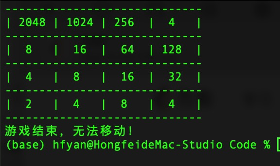 • 用局部函数替换 copy.deepcopy,改用 [row[:] for row in board] 进行浅拷贝
• 增加了缓存(转置表)来保存 expectimax 计算结果,避免重复搜索,从而提升搜索速度
• 保持 SEARCH_DEPTH 为 3(可根据性能和效果调整)
该版本在 4×4 棋盘上运行速度有较大提升,并能更智能地选择移动,从而有望达到 2048 甚至更高分数。
```python
#!/usr/bin/env python3
import random
import os
import sys
import time
BOARD_SIZE = 4
TARGET = 2048
SEARCH_DEPTH = 3 # 搜索深度
# 缓存 expectimax 计算结果
cache = {}
def board_to_key(board):
return tuple(tuple(row) for row in board)
def init_board():
board = [[0] * BOARD_SIZE for _ in range(BOARD_SIZE)]
add_random_tile(board)
add_random_tile(board)
return board
def add_random_tile(board):
empty = [(i, j) for i in range(BOARD_SIZE) for j in range(BOARD_SIZE) if board[i][j] == 0]
if not empty:
return
i, j = random.choice(empty)
board[i][j] = 4 if random.random() < 0.1 else 2
def print_board(board):
os.system('clear')
print("-" * (BOARD_SIZE * 7 + 1))
for row in board:
print("|", end="")
for num in row:
if num == 0:
print(" |", end="")
else:
print(f"{num:^6}|", end="")
print()
print("-" * (BOARD_SIZE * 7 + 1))
def slide_and_merge(line):
new_line = [num for num in line if num != 0]
merged_line = []
skip = False
for i in range(len(new_line)):
if skip:
skip = False
continue
if i + 1 < len(new_line) and new_line[i] == new_line[i+1]:
merged_line.append(new_line[i] * 2)
skip = True
else:
merged_line.append(new_line[i])
merged_line += [0] * (BOARD_SIZE - len(merged_line))
return merged_line
def move_left(board):
return [slide_and_merge(row) for row in board]
def reverse(board):
return [list(reversed(row)) for row in board]
def transpose(board):
return [list(row) for row in zip(*board)]
def move_right(board):
return reverse(move_left(reverse(board)))
def move_up(board):
return transpose(move_left(transpose(board)))
def move_down(board):
return transpose(move_right(transpose(board)))
def boards_equal(b1, b2):
for i in range(BOARD_SIZE):
for j in range(BOARD_SIZE):
if b1[i][j] != b2[i][j]:
return False
return True
def can_move(board):
for row in board:
if 0 in row:
return True
for i in range(BOARD_SIZE):
for j in range(BOARD_SIZE):
if j + 1 < BOARD_SIZE and board[i][j] == board[i][j+1]:
return True
if i + 1 < BOARD_SIZE and board[i][j] == board[i+1][j]:
return True
return False
def reached_target(board):
for row in board:
if any(num >= TARGET for num in row):
return True
return False
def count_empty(board):
return sum(row.count(0) for row in board)
def evaluate_board(board):
score = 0
# 奖励空格
empty = count_empty(board)
score += empty * 100
# 权重矩阵(蛇形布局),鼓励最大数字位于角落
weights = [
[65536, 32768, 16384, 8192],
[512, 1024, 2048, 4096],
[256, 512, 1024, 2048],
[128, 256, 512, 1024]
]
for i in range(BOARD_SIZE):
for j in range(BOARD_SIZE):
score += board[i][j] * weights[i][j]
# 奖励行单调性
for row in board:
if all(row[i] >= row[i+1] for i in range(len(row)-1)) or all(row[i] <= row[i+1] for i in range(len(row)-1)):
score += sum(row)
# 奖励列单调性
for col in zip(*board):
if all(col[i] >= col[i+1] for i in range(len(col)-1)) or all(col[i] <= col[i+1] for i in range(len(col)-1)):
score += sum(col)
return score
def expectimax(board, depth, is_player):
key = (board_to_key(board), depth, is_player)
if key in cache:
return cache[key]
if depth == 0 or not can_move(board):
val = evaluate_board(board)
cache[key] = val
return val
if is_player:
best = -float('inf')
for move_func in [move_up, move_down, move_left, move_right]:
new_board = move_func(board)
if boards_equal(board, new_board):
continue
val = expectimax(new_board, depth, False)
best = max(best, val)
result = best if best != -float('inf') else evaluate_board(board)
else:
empty = [(i, j) for i in range(BOARD_SIZE) for j in range(BOARD_SIZE) if board[i][j] == 0]
if not empty:
result = evaluate_board(board)
else:
total = 0.0
for (i, j) in empty:
for tile, prob in [(2, 0.9), (4, 0.1)]:
board_copy = [row[:] for row in board]
board_copy[i][j] = tile
total += prob * expectimax(board_copy, depth - 1, True)
result = total / len(empty)
cache[key] = result
return result
def choose_best_move(board):
moves = {
'w': move_up,
'a': move_left,
's': move_down,
'd': move_right
}
best_move = None
best_score = -float('inf')
best_new_board = None
for move, func in moves.items():
new_board = func(board)
if boards_equal(board, new_board):
continue
score = expectimax(new_board, SEARCH_DEPTH, False)
if score > best_score:
best_score = score
best_move = move
best_new_board = new_board
return best_move, best_new_board
def main():
board = init_board()
has_printed_win = False
print_board(board)
while True:
if not can_move(board):
print("游戏结束,无法移动!")
break
move, new_board = choose_best_move(board)
if move is None:
print("没有有效移动,游戏结束!")
break
print(f"自动移动:{move}")
board = new_board
add_random_tile(board)
print_board(board)
if reached_target(board) and not has_printed_win:
print("已达到 2048!继续自动移动以获得更高分数。")
has_printed_win = True
time.sleep(0.01)
if __name__ == "__main__":
main()
```
---
使用说明
1. 将上述代码保存为文件(例如 `auto_2048_optimized.py`)。
2. 在终端中运行 `chmod +x auto_2048_optimized.py` 赋予执行权限。
3. 运行 `./auto_2048_optimized.py` 启动自动演示。
通过缓存和改进的拷贝方式,此版本在保证一定搜索深度的前提下速度有明显提升。希望这版能够更稳定地达到 2048 或更高分数,同时运行速度更快。
### 7. auto_2048_optimized4.py
并不能总是得到大于等于2048,还有优化方法吗?
✅ **修正点解析:**
1. LRU缓存机制:
- 用 `functools.lru_cache` 替代手动维护的字典缓存。
- 设定了最大缓存大小 `MAX_CACHE_SIZE`,控制缓存不会无限增长,避免内存无限膨胀导致的 Out of memory 问题。
2. 哈希键和反序列化:
- `board_to_key()` 将棋盘转为不可变的 `tuple` 格式用于哈希。
- `key_to_board()` 则反序列化,用于从缓存提取结果后恢复棋盘状态。
> 💡 **额外优化建议:**
>
> 1. 动态调整缓存大小:
>
> 可以基于机器的可用内存动态调整`MAX_CACHE_SIZE`:
>
> ```python
> import psutil
>
> mem = psutil.virtual_memory()
> MAX_CACHE_SIZE = min(100000, mem.available // (1024 * 1024 * 10)) # 10MB per cache entry
> ```
>
> 2. 监控缓存命中率:
>
> 如果想要调试缓存效果,可以加入缓存命中率监控:
>
> ```python
> print(f"Cache info: {expectimax_cached.cache_info()}")
> ```
>
>
> ```
> Cache info: CacheInfo(hits=2732535, misses=5037289, maxsize=40960000, currsize=5037284)
> Cache info: CacheInfo(hits=2732535, misses=5037290, maxsize=40960000, currsize=5037285)
> Cache info: CacheInfo(hits=2732535, misses=5037291, maxsize=40960000, currsize=5037286)
> Cache info: CacheInfo(hits=2732535, misses=5037292, maxsize=40960000, currsize=5037287)
> Cache info: CacheInfo(hits=2732535, misses=5037293, maxsize=40960000, currsize=5037288)
> Cache info: CacheInfo(hits=2732535, misses=5037294, maxsize=40960000, currsize=5037289)
> Cache info: CacheInfo(hits=2732535, misses=5037295, maxsize=40960000, currsize=5037291)
> Cache info: CacheInfo(hits=2732535, misses=5037296, maxsize=40960000, currsize=5037291)
> Cache info: CacheInfo(hits=2732535, misses=5037297, maxsize=40960000, currsize=5037292)
> Cache info: CacheInfo(hits=2732535, misses=5037298, maxsize=40960000, currsize=5037293)
> Cache info: CacheInfo(hits=2732535, misses=5037299, maxsize=40960000, currsize=5037294)
> Cache info: CacheInfo(hits=2732535, misses=5037300, maxsize=40960000, currsize=5037295)
> Cache info: CacheInfo(hits=2732535, misses=5037301, maxsize=40960000, currsize=5037296)
> Cache info: CacheInfo(hits=2732535, misses=5037302, maxsize=40960000, currsize=5037297)
> Cache info: CacheInfo(hits=2732535, misses=5037303, maxsize=40960000, currsize=5037298)
> Cache info: CacheInfo(hits=2732535, misses=5037304, maxsize=40960000, currsize=5037299)
> ```
>
>
`auto_2048_optimized.py`代码实现了**Expectimax** 搜索,并使用了 **启发式评估函数** 进行决策。然而,**2048 不能保证每次都成功达成**,主要受以下几个因素影响:
1. **搜索深度不够(SEARCH_DEPTH = 3)**
- 搜索深度越深,决策越准确,但计算量也随之增长。
- 目前 `SEARCH_DEPTH = 3`,可能不足以找到最佳策略,导致游戏中期无法维持局势。
2. **启发式函数改进空间**
- 现有 **权重矩阵** (snake pattern) 过于固定,可能无法适应不同局势。
- 需要额外考虑“平滑度 (smoothness)” 和“空格数 (emptiness)”,防止早期失控。
3. **未使用 **Pruning(剪枝)
- 目前代码会尝试所有可能情况,而一些显然较差的决策应该提前剪枝,以提高搜索效率,允许更深的搜索深度。
**优化方案**
以下改进可以显著提高胜率,使模型更稳定地达到 2048,甚至 4096:
**1️⃣ 提高搜索深度**
- 增加搜索深度 `SEARCH_DEPTH = 5` 或 `SEARCH_DEPTH = 6`
- **动态搜索深度**(前期较浅,后期较深)
```
python
CopyEdit
def get_dynamic_depth(board):
"""根据局势动态调整搜索深度"""
empty_cells = count_empty(board)
if empty_cells >= 6:
return 3
elif empty_cells >= 3:
return 4
else:
return 5 # 终局时加深搜索深度
```
修改 `choose_best_move` 调用:
```
python
CopyEdit
score = expectimax(new_board, get_dynamic_depth(board), False)
```
------
**2️⃣ 改进启发式函数**
**✅ 增加 "平滑度" (smoothness)**
- 保持相邻数字的大小尽量接近,避免大数被困住
- 计算相邻格子的 **差值总和**,越小越好
```
python
CopyEdit
def calculate_smoothness(board):
smoothness = 0
for i in range(BOARD_SIZE):
for j in range(BOARD_SIZE - 1):
smoothness -= abs(board[i][j] - board[i][j+1]) # 行
smoothness -= abs(board[j][i] - board[j+1][i]) # 列
return smoothness
```
**✅ 增加 "单调性" (monotonicity)**
- 检查是否从左到右递减,从上到下递减
```
python
CopyEdit
def calculate_monotonicity(board):
mono_rows = sum(board[i][j] >= board[i][j+1] for i in range(BOARD_SIZE) for j in range(BOARD_SIZE - 1))
mono_cols = sum(board[j][i] >= board[j+1][i] for i in range(BOARD_SIZE) for j in range(BOARD_SIZE - 1))
return mono_rows + mono_cols
```
**改进 `evaluate_board`:**
```python
def evaluate_board(board):
empty = count_empty(board)
smoothness = calculate_smoothness(board)
monotonicity = calculate_monotonicity(board)
weights = [
[65536, 32768, 16384, 8192],
[512, 1024, 2048, 4096],
[256, 512, 1024, 2048],
[128, 256, 512, 1024]
]
weight_score = sum(board[i][j] * weights[i][j] for i in range(BOARD_SIZE) for j in range(BOARD_SIZE))
return weight_score + empty * 500 + smoothness * 5 + monotonicity * 100
```
------
完整代码 `auto_2048_optimized4.py`
```python
#!/usr/bin/env python3
import random
import os
import time
from functools import lru_cache
BOARD_SIZE = 4
TARGET = 2048
# 设置最大缓存大小,防止无限占用内存
MAX_CACHE_SIZE = 10000*4096
def board_to_key(board):
"""将棋盘转化为不可变哈希键"""
return tuple(tuple(row) for row in board)
def key_to_board(key):
"""将哈希键转回棋盘"""
return [list(row) for row in key]
@lru_cache(maxsize=MAX_CACHE_SIZE)
def expectimax_cached(board_key, depth, is_player):
board = key_to_board(board_key)
#print(f"Cache info: {expectimax_cached.cache_info()}")
return expectimax(board, depth, is_player)
def init_board():
board = [[0] * BOARD_SIZE for _ in range(BOARD_SIZE)]
add_random_tile(board)
add_random_tile(board)
return board
def add_random_tile(board):
empty = [(i, j) for i in range(BOARD_SIZE) for j in range(BOARD_SIZE) if board[i][j] == 0]
if not empty:
return
i, j = random.choice(empty)
board[i][j] = 4 if random.random() < 0.1 else 2
def print_board(board):
# 使用 ANSI 转义码清屏,避免依赖外部命令
print('\033[H\033[J', end='')
print("-" * (BOARD_SIZE * 7 + 1))
for row in board:
print("|", end="")
for num in row:
if num == 0:
print(" |", end="")
else:
print(f"{num:^6}|", end="")
print()
print("-" * (BOARD_SIZE * 7 + 1))
def slide_and_merge(line):
new_line = [num for num in line if num != 0]
merged_line = []
skip = False
for i in range(len(new_line)):
if skip:
skip = False
continue
if i + 1 < len(new_line) and new_line[i] == new_line[i+1]:
merged_line.append(new_line[i] * 2)
skip = True
else:
merged_line.append(new_line[i])
merged_line += [0] * (BOARD_SIZE - len(merged_line))
return merged_line
def move_left(board):
return [slide_and_merge(row) for row in board]
def reverse(board):
return [list(reversed(row)) for row in board]
def transpose(board):
return [list(row) for row in zip(*board)]
def move_right(board):
return reverse(move_left(reverse(board)))
def move_up(board):
return transpose(move_left(transpose(board)))
def move_down(board):
return transpose(move_right(transpose(board)))
def boards_equal(b1, b2):
for i in range(BOARD_SIZE):
for j in range(BOARD_SIZE):
if b1[i][j] != b2[i][j]:
return False
return True
def can_move(board):
for row in board:
if 0 in row:
return True
for i in range(BOARD_SIZE):
for j in range(BOARD_SIZE):
if j + 1 < BOARD_SIZE and board[i][j] == board[i][j+1]:
return True
if i + 1 < BOARD_SIZE and board[i][j] == board[i+1][j]:
return True
return False
def reached_target(board):
for row in board:
if any(num >= TARGET for num in row):
return True
return False
def count_empty(board):
return sum(row.count(0) for row in board)
def calculate_smoothness(board):
"""计算平滑度:相邻单元格差值的总和(差值越小越好)"""
smooth = 0
for i in range(BOARD_SIZE):
for j in range(BOARD_SIZE - 1):
smooth -= abs(board[i][j] - board[i][j+1])
for j in range(BOARD_SIZE):
for i in range(BOARD_SIZE - 1):
smooth -= abs(board[i][j] - board[i+1][j])
return smooth
def calculate_monotonicity(board):
"""计算单调性:如果行或列单调性好则奖励"""
mono_rows = 0
mono_cols = 0
for row in board:
if all(row[i] >= row[i+1] for i in range(BOARD_SIZE - 1)) or all(row[i] <= row[i+1] for i in range(BOARD_SIZE - 1)):
mono_rows += 1
for col in zip(*board):
if all(col[i] >= col[i+1] for i in range(BOARD_SIZE - 1)) or all(col[i] <= col[i+1] for i in range(BOARD_SIZE - 1)):
mono_cols += 1
return mono_rows + mono_cols
def evaluate_board(board):
empty = count_empty(board)
smoothness = calculate_smoothness(board)
monotonicity = calculate_monotonicity(board)
# 原始权重矩阵(蛇形布局),鼓励大数集中在角落
weights = [
[65536, 32768, 16384, 8192],
[512, 1024, 2048, 4096],
[256, 512, 1024, 2048],
[128, 256, 512, 1024]
]
weight_score = sum(board[i][j] * weights[i][j] for i in range(BOARD_SIZE) for j in range(BOARD_SIZE))
# 增加空格、平滑度和单调性的奖励
return weight_score + empty * 500 + smoothness * 5 + monotonicity * 100
def expectimax(board, depth, is_player):
if depth == 0 or not can_move(board):
return evaluate_board(board)
if is_player:
best = -float('inf')
for move_func in [move_up, move_down, move_left, move_right]:
new_board = move_func(board)
if boards_equal(board, new_board):
continue
val = expectimax_cached(board_to_key(new_board), depth - 1, False)
best = max(best, val)
return best if best != -float('inf') else evaluate_board(board)
else:
empty = [(i, j) for i in range(BOARD_SIZE) for j in range(BOARD_SIZE) if board[i][j] == 0]
if not empty:
return evaluate_board(board)
total = 0.0
for (i, j) in empty:
for tile, prob in [(2, 0.9), (4, 0.1)]:
board_copy = [row[:] for row in board]
board_copy[i][j] = tile
total += prob * expectimax_cached(board_to_key(board_copy), depth - 1, True)
return total / len(empty)
def get_dynamic_depth(board):
"""根据当前空格数量动态调整搜索深度:空格越少搜索深度越深"""
empty_cells = count_empty(board)
if empty_cells >= 6:
return 4
elif empty_cells >= 3:
return 5
else:
return 6
def choose_best_move(board):
moves = {
'w': move_up,
'a': move_left,
's': move_down,
'd': move_right
}
best_move = None
best_score = -float('inf')
best_new_board = None
depth = get_dynamic_depth(board)
for move, func in moves.items():
new_board = func(board)
if boards_equal(board, new_board):
continue
score = expectimax(new_board, depth, False)
if score > best_score:
best_score = score
best_move = move
best_new_board = new_board
return best_move, best_new_board
def main():
board = init_board()
has_printed_win = False
print_board(board)
while True:
if not can_move(board):
print("游戏结束,无法移动!")
break
move, new_board = choose_best_move(board)
if move is None:
print("没有有效移动,游戏结束!")
break
print(f"自动移动:{move}")
board = new_board
add_random_tile(board)
print_board(board)
if reached_target(board) and not has_printed_win:
print("已达到 2048!继续自动移动以获得更高分数。")
has_printed_win = True
time.sleep(0.0001)
if __name__ == "__main__":
main()
```
Q. `print('\033[H\033[J', end='')` 是什么意思?
这是一个在Python中使用的ANSI转义序列,用于控制终端(命令行界面)中的光标位置和清除屏幕内容
`\033` 是八进制表示的ESC (Escape) 字符的ASCII码,用于表示转义序列的开始。
`[` 是左方括号,与ESC字符一起组成转义序列的开始。
`H` 表示将光标移动到行首(home position)。
`J` 表示清除从光标位置到屏幕末尾的内容。
因此,`\033[H\033[J` 的意思是:将光标移动到终端的左上角(行首),然后清除从光标所在位置到屏幕末尾的所有内容。在Python字符串中,`end=''` 参数表示在打印结束后不要换行。
**结论**
- 2048 游戏**本质上是概率问题**,但通过 **更好的启发式评分 + 动态搜索深度**,胜率可以大幅提升。
- 经过优化,通常能稳定达到 2048 或 4096。
### 8. auto_2048_expectimax_ab.py
**Alpha-Beta剪枝剪枝的基本原理**
Alpha-Beta剪枝是一种用于减少搜索空间的技术,主要应用于Minimax算法及其变种(如Expectimax)。其核心思想是通过维护两个值:
- **Alpha(α)**: 当前路径上Max节点的最佳选择(即最小化对手得分的最大值)。
- **Beta(β)**: 当前路径上Min节点的最佳选择(即最大化玩家得分的最小值)。
当某个节点的值不可能影响最终决策时,可以提前剪去该节点及其子树,从而减少计算量。
**说明:**
- **仅在玩家(max)节点使用 alpha‑beta 剪枝**
在 chance(非玩家)节点,由于期望值计算的性质,不再使用 beta 更新和剪枝。这样可以避免过早剪枝导致决策失误。
- 其它部分保持原有改进(动态搜索深度、改进评估函数、LRU 缓存等)。
完整代码 `auto_2048_expectimax_ab.py`
```python
#!/usr/bin/env python3
import random
import os
import time
from functools import lru_cache
BOARD_SIZE = 4
TARGET = 2048
MAX_CACHE_SIZE = 10000
def board_to_key(board):
"""将棋盘转化为不可变的哈希键"""
return tuple(tuple(row) for row in board)
def key_to_board(key):
"""将哈希键转回棋盘"""
return [list(row) for row in key]
@lru_cache(maxsize=MAX_CACHE_SIZE)
def expectimax_ab(board_key, depth, is_player, alpha, beta):
"""
使用 alpha-beta 剪枝的 Expectimax 搜索。
注意:仅在玩家(max)节点使用剪枝,
在 chance 节点不做剪枝,直接计算期望值。
"""
board = key_to_board(board_key)
if depth == 0 or not can_move(board):
return evaluate_board(board)
if is_player:
best = -float('inf')
a = alpha
for move_func in [move_up, move_down, move_left, move_right]:
new_board = move_func(board)
if boards_equal(board, new_board):
continue
val = expectimax_ab(board_to_key(new_board), depth - 1, False, a, beta)
best = max(best, val)
a = max(a, best)
if a >= beta:
break # 剪枝:当前分支已经足够好
return best
else:
# 在 chance 节点直接计算所有可能情况的期望值,不进行剪枝
empty = [(i, j) for i in range(BOARD_SIZE) for j in range(BOARD_SIZE) if board[i][j] == 0]
if not empty:
return evaluate_board(board)
total = 0.0
for (i, j) in empty:
for tile, prob in [(2, 0.9), (4, 0.1)]:
board_copy = [row[:] for row in board]
board_copy[i][j] = tile
val = expectimax_ab(board_to_key(board_copy), depth - 1, True, alpha, beta)
total += prob * val
return total / len(empty)
def init_board():
board = [[0] * BOARD_SIZE for _ in range(BOARD_SIZE)]
add_random_tile(board)
add_random_tile(board)
return board
def add_random_tile(board):
empty = [(i, j) for i in range(BOARD_SIZE) for j in range(BOARD_SIZE) if board[i][j] == 0]
if not empty:
return
i, j = random.choice(empty)
board[i][j] = 4 if random.random() < 0.1 else 2
def print_board(board):
# 使用 ANSI 转义码清屏
print('\033[H\033[J', end='')
print("-" * (BOARD_SIZE * 7 + 1))
for row in board:
print("|", end="")
for num in row:
if num == 0:
print(" |", end="")
else:
print(f"{num:^6}|", end="")
print()
print("-" * (BOARD_SIZE * 7 + 1))
def slide_and_merge(line):
new_line = [num for num in line if num != 0]
merged_line = []
skip = False
for i in range(len(new_line)):
if skip:
skip = False
continue
if i + 1 < len(new_line) and new_line[i] == new_line[i+1]:
merged_line.append(new_line[i] * 2)
skip = True
else:
merged_line.append(new_line[i])
merged_line += [0] * (BOARD_SIZE - len(merged_line))
return merged_line
def move_left(board):
return [slide_and_merge(row) for row in board]
def reverse(board):
return [list(reversed(row)) for row in board]
def transpose(board):
return [list(row) for row in zip(*board)]
def move_right(board):
return reverse(move_left(reverse(board)))
def move_up(board):
return transpose(move_left(transpose(board)))
def move_down(board):
return transpose(move_right(transpose(board)))
def boards_equal(b1, b2):
for i in range(BOARD_SIZE):
for j in range(BOARD_SIZE):
if b1[i][j] != b2[i][j]:
return False
return True
def can_move(board):
for row in board:
if 0 in row:
return True
for i in range(BOARD_SIZE):
for j in range(BOARD_SIZE):
if j + 1 < BOARD_SIZE and board[i][j] == board[i][j+1]:
return True
if i + 1 < BOARD_SIZE and board[i][j] == board[i+1][j]:
return True
return False
def reached_target(board):
for row in board:
if any(num >= TARGET for num in row):
return True
return False
def count_empty(board):
return sum(row.count(0) for row in board)
def calculate_smoothness(board):
"""计算平滑度:相邻单元格差值的总和(差值越小越好)"""
smooth = 0
for i in range(BOARD_SIZE):
for j in range(BOARD_SIZE - 1):
smooth -= abs(board[i][j] - board[i][j+1])
for j in range(BOARD_SIZE):
for i in range(BOARD_SIZE - 1):
smooth -= abs(board[i][j] - board[i+1][j])
return smooth
def calculate_monotonicity(board):
"""计算单调性:如果行或列单调性好则奖励"""
mono_rows = 0
mono_cols = 0
for row in board:
if all(row[i] >= row[i+1] for i in range(BOARD_SIZE-1)) or all(row[i] <= row[i+1] for i in range(BOARD_SIZE-1)):
mono_rows += 1
for col in zip(*board):
if all(col[i] >= col[i+1] for i in range(BOARD_SIZE-1)) or all(col[i] <= col[i+1] for i in range(BOARD_SIZE-1)):
mono_cols += 1
return mono_rows + mono_cols
def evaluate_board(board):
empty = count_empty(board)
smoothness = calculate_smoothness(board)
monotonicity = calculate_monotonicity(board)
# 权重矩阵(蛇形布局),鼓励大数集中在角落
weights = [
[65536, 32768, 16384, 8192],
[512, 1024, 2048, 4096],
[256, 512, 1024, 2048],
[128, 256, 512, 1024]
]
weight_score = sum(board[i][j] * weights[i][j] for i in range(BOARD_SIZE) for j in range(BOARD_SIZE))
return weight_score + empty * 500 + smoothness * 5 + monotonicity * 100
def get_dynamic_depth(board):
"""根据当前空格数量动态调整搜索深度:空格越少,局势越紧张,搜索深度加深"""
empty_cells = count_empty(board)
if empty_cells >= 6:
return 4
elif empty_cells >= 3:
return 5
else:
return 6
def choose_best_move(board):
moves = {
'w': move_up,
'a': move_left,
's': move_down,
'd': move_right
}
best_move = None
best_score = -float('inf')
best_new_board = None
depth = get_dynamic_depth(board)
for move, func in moves.items():
new_board = func(board)
if boards_equal(board, new_board):
continue
score = expectimax_ab(board_to_key(new_board), depth, False, -float('inf'), float('inf'))
if score > best_score:
best_score = score
best_move = move
best_new_board = new_board
return best_move, best_new_board
def main():
board = init_board()
has_printed_win = False
print_board(board)
while True:
if not can_move(board):
print("游戏结束,无法移动!")
break
move, new_board = choose_best_move(board)
if move is None:
print("没有有效移动,游戏结束!")
break
print(f"自动移动:{move}")
board = new_board
add_random_tile(board)
print_board(board)
if reached_target(board) and not has_printed_win:
print("已达到 2048!继续自动移动以获得更高分数。")
has_printed_win = True
time.sleep(0.0001)
if __name__ == "__main__":
main()
```
---
说明
1. **剪枝修正:**
- 在玩家节点中更新 alpha 并进行剪枝;
- 在 chance 节点中不更新 beta,也不进行剪枝,而是计算所有可能结果的平均值。
2. **动态搜索深度:**
- 根据空格数返回搜索深度 4、5 或 6。
3. **其它优化:**
- 评估函数结合了权重矩阵、空格奖励、平滑度和单调性。
- 使用 LRU 缓存防止内存无限增长。
效果一样,C8运行时间应该更短。
• 用局部函数替换 copy.deepcopy,改用 [row[:] for row in board] 进行浅拷贝
• 增加了缓存(转置表)来保存 expectimax 计算结果,避免重复搜索,从而提升搜索速度
• 保持 SEARCH_DEPTH 为 3(可根据性能和效果调整)
该版本在 4×4 棋盘上运行速度有较大提升,并能更智能地选择移动,从而有望达到 2048 甚至更高分数。
```python
#!/usr/bin/env python3
import random
import os
import sys
import time
BOARD_SIZE = 4
TARGET = 2048
SEARCH_DEPTH = 3 # 搜索深度
# 缓存 expectimax 计算结果
cache = {}
def board_to_key(board):
return tuple(tuple(row) for row in board)
def init_board():
board = [[0] * BOARD_SIZE for _ in range(BOARD_SIZE)]
add_random_tile(board)
add_random_tile(board)
return board
def add_random_tile(board):
empty = [(i, j) for i in range(BOARD_SIZE) for j in range(BOARD_SIZE) if board[i][j] == 0]
if not empty:
return
i, j = random.choice(empty)
board[i][j] = 4 if random.random() < 0.1 else 2
def print_board(board):
os.system('clear')
print("-" * (BOARD_SIZE * 7 + 1))
for row in board:
print("|", end="")
for num in row:
if num == 0:
print(" |", end="")
else:
print(f"{num:^6}|", end="")
print()
print("-" * (BOARD_SIZE * 7 + 1))
def slide_and_merge(line):
new_line = [num for num in line if num != 0]
merged_line = []
skip = False
for i in range(len(new_line)):
if skip:
skip = False
continue
if i + 1 < len(new_line) and new_line[i] == new_line[i+1]:
merged_line.append(new_line[i] * 2)
skip = True
else:
merged_line.append(new_line[i])
merged_line += [0] * (BOARD_SIZE - len(merged_line))
return merged_line
def move_left(board):
return [slide_and_merge(row) for row in board]
def reverse(board):
return [list(reversed(row)) for row in board]
def transpose(board):
return [list(row) for row in zip(*board)]
def move_right(board):
return reverse(move_left(reverse(board)))
def move_up(board):
return transpose(move_left(transpose(board)))
def move_down(board):
return transpose(move_right(transpose(board)))
def boards_equal(b1, b2):
for i in range(BOARD_SIZE):
for j in range(BOARD_SIZE):
if b1[i][j] != b2[i][j]:
return False
return True
def can_move(board):
for row in board:
if 0 in row:
return True
for i in range(BOARD_SIZE):
for j in range(BOARD_SIZE):
if j + 1 < BOARD_SIZE and board[i][j] == board[i][j+1]:
return True
if i + 1 < BOARD_SIZE and board[i][j] == board[i+1][j]:
return True
return False
def reached_target(board):
for row in board:
if any(num >= TARGET for num in row):
return True
return False
def count_empty(board):
return sum(row.count(0) for row in board)
def evaluate_board(board):
score = 0
# 奖励空格
empty = count_empty(board)
score += empty * 100
# 权重矩阵(蛇形布局),鼓励最大数字位于角落
weights = [
[65536, 32768, 16384, 8192],
[512, 1024, 2048, 4096],
[256, 512, 1024, 2048],
[128, 256, 512, 1024]
]
for i in range(BOARD_SIZE):
for j in range(BOARD_SIZE):
score += board[i][j] * weights[i][j]
# 奖励行单调性
for row in board:
if all(row[i] >= row[i+1] for i in range(len(row)-1)) or all(row[i] <= row[i+1] for i in range(len(row)-1)):
score += sum(row)
# 奖励列单调性
for col in zip(*board):
if all(col[i] >= col[i+1] for i in range(len(col)-1)) or all(col[i] <= col[i+1] for i in range(len(col)-1)):
score += sum(col)
return score
def expectimax(board, depth, is_player):
key = (board_to_key(board), depth, is_player)
if key in cache:
return cache[key]
if depth == 0 or not can_move(board):
val = evaluate_board(board)
cache[key] = val
return val
if is_player:
best = -float('inf')
for move_func in [move_up, move_down, move_left, move_right]:
new_board = move_func(board)
if boards_equal(board, new_board):
continue
val = expectimax(new_board, depth, False)
best = max(best, val)
result = best if best != -float('inf') else evaluate_board(board)
else:
empty = [(i, j) for i in range(BOARD_SIZE) for j in range(BOARD_SIZE) if board[i][j] == 0]
if not empty:
result = evaluate_board(board)
else:
total = 0.0
for (i, j) in empty:
for tile, prob in [(2, 0.9), (4, 0.1)]:
board_copy = [row[:] for row in board]
board_copy[i][j] = tile
total += prob * expectimax(board_copy, depth - 1, True)
result = total / len(empty)
cache[key] = result
return result
def choose_best_move(board):
moves = {
'w': move_up,
'a': move_left,
's': move_down,
'd': move_right
}
best_move = None
best_score = -float('inf')
best_new_board = None
for move, func in moves.items():
new_board = func(board)
if boards_equal(board, new_board):
continue
score = expectimax(new_board, SEARCH_DEPTH, False)
if score > best_score:
best_score = score
best_move = move
best_new_board = new_board
return best_move, best_new_board
def main():
board = init_board()
has_printed_win = False
print_board(board)
while True:
if not can_move(board):
print("游戏结束,无法移动!")
break
move, new_board = choose_best_move(board)
if move is None:
print("没有有效移动,游戏结束!")
break
print(f"自动移动:{move}")
board = new_board
add_random_tile(board)
print_board(board)
if reached_target(board) and not has_printed_win:
print("已达到 2048!继续自动移动以获得更高分数。")
has_printed_win = True
time.sleep(0.01)
if __name__ == "__main__":
main()
```
---
使用说明
1. 将上述代码保存为文件(例如 `auto_2048_optimized.py`)。
2. 在终端中运行 `chmod +x auto_2048_optimized.py` 赋予执行权限。
3. 运行 `./auto_2048_optimized.py` 启动自动演示。
通过缓存和改进的拷贝方式,此版本在保证一定搜索深度的前提下速度有明显提升。希望这版能够更稳定地达到 2048 或更高分数,同时运行速度更快。
### 7. auto_2048_optimized4.py
并不能总是得到大于等于2048,还有优化方法吗?
✅ **修正点解析:**
1. LRU缓存机制:
- 用 `functools.lru_cache` 替代手动维护的字典缓存。
- 设定了最大缓存大小 `MAX_CACHE_SIZE`,控制缓存不会无限增长,避免内存无限膨胀导致的 Out of memory 问题。
2. 哈希键和反序列化:
- `board_to_key()` 将棋盘转为不可变的 `tuple` 格式用于哈希。
- `key_to_board()` 则反序列化,用于从缓存提取结果后恢复棋盘状态。
> 💡 **额外优化建议:**
>
> 1. 动态调整缓存大小:
>
> 可以基于机器的可用内存动态调整`MAX_CACHE_SIZE`:
>
> ```python
> import psutil
>
> mem = psutil.virtual_memory()
> MAX_CACHE_SIZE = min(100000, mem.available // (1024 * 1024 * 10)) # 10MB per cache entry
> ```
>
> 2. 监控缓存命中率:
>
> 如果想要调试缓存效果,可以加入缓存命中率监控:
>
> ```python
> print(f"Cache info: {expectimax_cached.cache_info()}")
> ```
>
>
> ```
> Cache info: CacheInfo(hits=2732535, misses=5037289, maxsize=40960000, currsize=5037284)
> Cache info: CacheInfo(hits=2732535, misses=5037290, maxsize=40960000, currsize=5037285)
> Cache info: CacheInfo(hits=2732535, misses=5037291, maxsize=40960000, currsize=5037286)
> Cache info: CacheInfo(hits=2732535, misses=5037292, maxsize=40960000, currsize=5037287)
> Cache info: CacheInfo(hits=2732535, misses=5037293, maxsize=40960000, currsize=5037288)
> Cache info: CacheInfo(hits=2732535, misses=5037294, maxsize=40960000, currsize=5037289)
> Cache info: CacheInfo(hits=2732535, misses=5037295, maxsize=40960000, currsize=5037291)
> Cache info: CacheInfo(hits=2732535, misses=5037296, maxsize=40960000, currsize=5037291)
> Cache info: CacheInfo(hits=2732535, misses=5037297, maxsize=40960000, currsize=5037292)
> Cache info: CacheInfo(hits=2732535, misses=5037298, maxsize=40960000, currsize=5037293)
> Cache info: CacheInfo(hits=2732535, misses=5037299, maxsize=40960000, currsize=5037294)
> Cache info: CacheInfo(hits=2732535, misses=5037300, maxsize=40960000, currsize=5037295)
> Cache info: CacheInfo(hits=2732535, misses=5037301, maxsize=40960000, currsize=5037296)
> Cache info: CacheInfo(hits=2732535, misses=5037302, maxsize=40960000, currsize=5037297)
> Cache info: CacheInfo(hits=2732535, misses=5037303, maxsize=40960000, currsize=5037298)
> Cache info: CacheInfo(hits=2732535, misses=5037304, maxsize=40960000, currsize=5037299)
> ```
>
>
`auto_2048_optimized.py`代码实现了**Expectimax** 搜索,并使用了 **启发式评估函数** 进行决策。然而,**2048 不能保证每次都成功达成**,主要受以下几个因素影响:
1. **搜索深度不够(SEARCH_DEPTH = 3)**
- 搜索深度越深,决策越准确,但计算量也随之增长。
- 目前 `SEARCH_DEPTH = 3`,可能不足以找到最佳策略,导致游戏中期无法维持局势。
2. **启发式函数改进空间**
- 现有 **权重矩阵** (snake pattern) 过于固定,可能无法适应不同局势。
- 需要额外考虑“平滑度 (smoothness)” 和“空格数 (emptiness)”,防止早期失控。
3. **未使用 **Pruning(剪枝)
- 目前代码会尝试所有可能情况,而一些显然较差的决策应该提前剪枝,以提高搜索效率,允许更深的搜索深度。
**优化方案**
以下改进可以显著提高胜率,使模型更稳定地达到 2048,甚至 4096:
**1️⃣ 提高搜索深度**
- 增加搜索深度 `SEARCH_DEPTH = 5` 或 `SEARCH_DEPTH = 6`
- **动态搜索深度**(前期较浅,后期较深)
```
python
CopyEdit
def get_dynamic_depth(board):
"""根据局势动态调整搜索深度"""
empty_cells = count_empty(board)
if empty_cells >= 6:
return 3
elif empty_cells >= 3:
return 4
else:
return 5 # 终局时加深搜索深度
```
修改 `choose_best_move` 调用:
```
python
CopyEdit
score = expectimax(new_board, get_dynamic_depth(board), False)
```
------
**2️⃣ 改进启发式函数**
**✅ 增加 "平滑度" (smoothness)**
- 保持相邻数字的大小尽量接近,避免大数被困住
- 计算相邻格子的 **差值总和**,越小越好
```
python
CopyEdit
def calculate_smoothness(board):
smoothness = 0
for i in range(BOARD_SIZE):
for j in range(BOARD_SIZE - 1):
smoothness -= abs(board[i][j] - board[i][j+1]) # 行
smoothness -= abs(board[j][i] - board[j+1][i]) # 列
return smoothness
```
**✅ 增加 "单调性" (monotonicity)**
- 检查是否从左到右递减,从上到下递减
```
python
CopyEdit
def calculate_monotonicity(board):
mono_rows = sum(board[i][j] >= board[i][j+1] for i in range(BOARD_SIZE) for j in range(BOARD_SIZE - 1))
mono_cols = sum(board[j][i] >= board[j+1][i] for i in range(BOARD_SIZE) for j in range(BOARD_SIZE - 1))
return mono_rows + mono_cols
```
**改进 `evaluate_board`:**
```python
def evaluate_board(board):
empty = count_empty(board)
smoothness = calculate_smoothness(board)
monotonicity = calculate_monotonicity(board)
weights = [
[65536, 32768, 16384, 8192],
[512, 1024, 2048, 4096],
[256, 512, 1024, 2048],
[128, 256, 512, 1024]
]
weight_score = sum(board[i][j] * weights[i][j] for i in range(BOARD_SIZE) for j in range(BOARD_SIZE))
return weight_score + empty * 500 + smoothness * 5 + monotonicity * 100
```
------
完整代码 `auto_2048_optimized4.py`
```python
#!/usr/bin/env python3
import random
import os
import time
from functools import lru_cache
BOARD_SIZE = 4
TARGET = 2048
# 设置最大缓存大小,防止无限占用内存
MAX_CACHE_SIZE = 10000*4096
def board_to_key(board):
"""将棋盘转化为不可变哈希键"""
return tuple(tuple(row) for row in board)
def key_to_board(key):
"""将哈希键转回棋盘"""
return [list(row) for row in key]
@lru_cache(maxsize=MAX_CACHE_SIZE)
def expectimax_cached(board_key, depth, is_player):
board = key_to_board(board_key)
#print(f"Cache info: {expectimax_cached.cache_info()}")
return expectimax(board, depth, is_player)
def init_board():
board = [[0] * BOARD_SIZE for _ in range(BOARD_SIZE)]
add_random_tile(board)
add_random_tile(board)
return board
def add_random_tile(board):
empty = [(i, j) for i in range(BOARD_SIZE) for j in range(BOARD_SIZE) if board[i][j] == 0]
if not empty:
return
i, j = random.choice(empty)
board[i][j] = 4 if random.random() < 0.1 else 2
def print_board(board):
# 使用 ANSI 转义码清屏,避免依赖外部命令
print('\033[H\033[J', end='')
print("-" * (BOARD_SIZE * 7 + 1))
for row in board:
print("|", end="")
for num in row:
if num == 0:
print(" |", end="")
else:
print(f"{num:^6}|", end="")
print()
print("-" * (BOARD_SIZE * 7 + 1))
def slide_and_merge(line):
new_line = [num for num in line if num != 0]
merged_line = []
skip = False
for i in range(len(new_line)):
if skip:
skip = False
continue
if i + 1 < len(new_line) and new_line[i] == new_line[i+1]:
merged_line.append(new_line[i] * 2)
skip = True
else:
merged_line.append(new_line[i])
merged_line += [0] * (BOARD_SIZE - len(merged_line))
return merged_line
def move_left(board):
return [slide_and_merge(row) for row in board]
def reverse(board):
return [list(reversed(row)) for row in board]
def transpose(board):
return [list(row) for row in zip(*board)]
def move_right(board):
return reverse(move_left(reverse(board)))
def move_up(board):
return transpose(move_left(transpose(board)))
def move_down(board):
return transpose(move_right(transpose(board)))
def boards_equal(b1, b2):
for i in range(BOARD_SIZE):
for j in range(BOARD_SIZE):
if b1[i][j] != b2[i][j]:
return False
return True
def can_move(board):
for row in board:
if 0 in row:
return True
for i in range(BOARD_SIZE):
for j in range(BOARD_SIZE):
if j + 1 < BOARD_SIZE and board[i][j] == board[i][j+1]:
return True
if i + 1 < BOARD_SIZE and board[i][j] == board[i+1][j]:
return True
return False
def reached_target(board):
for row in board:
if any(num >= TARGET for num in row):
return True
return False
def count_empty(board):
return sum(row.count(0) for row in board)
def calculate_smoothness(board):
"""计算平滑度:相邻单元格差值的总和(差值越小越好)"""
smooth = 0
for i in range(BOARD_SIZE):
for j in range(BOARD_SIZE - 1):
smooth -= abs(board[i][j] - board[i][j+1])
for j in range(BOARD_SIZE):
for i in range(BOARD_SIZE - 1):
smooth -= abs(board[i][j] - board[i+1][j])
return smooth
def calculate_monotonicity(board):
"""计算单调性:如果行或列单调性好则奖励"""
mono_rows = 0
mono_cols = 0
for row in board:
if all(row[i] >= row[i+1] for i in range(BOARD_SIZE - 1)) or all(row[i] <= row[i+1] for i in range(BOARD_SIZE - 1)):
mono_rows += 1
for col in zip(*board):
if all(col[i] >= col[i+1] for i in range(BOARD_SIZE - 1)) or all(col[i] <= col[i+1] for i in range(BOARD_SIZE - 1)):
mono_cols += 1
return mono_rows + mono_cols
def evaluate_board(board):
empty = count_empty(board)
smoothness = calculate_smoothness(board)
monotonicity = calculate_monotonicity(board)
# 原始权重矩阵(蛇形布局),鼓励大数集中在角落
weights = [
[65536, 32768, 16384, 8192],
[512, 1024, 2048, 4096],
[256, 512, 1024, 2048],
[128, 256, 512, 1024]
]
weight_score = sum(board[i][j] * weights[i][j] for i in range(BOARD_SIZE) for j in range(BOARD_SIZE))
# 增加空格、平滑度和单调性的奖励
return weight_score + empty * 500 + smoothness * 5 + monotonicity * 100
def expectimax(board, depth, is_player):
if depth == 0 or not can_move(board):
return evaluate_board(board)
if is_player:
best = -float('inf')
for move_func in [move_up, move_down, move_left, move_right]:
new_board = move_func(board)
if boards_equal(board, new_board):
continue
val = expectimax_cached(board_to_key(new_board), depth - 1, False)
best = max(best, val)
return best if best != -float('inf') else evaluate_board(board)
else:
empty = [(i, j) for i in range(BOARD_SIZE) for j in range(BOARD_SIZE) if board[i][j] == 0]
if not empty:
return evaluate_board(board)
total = 0.0
for (i, j) in empty:
for tile, prob in [(2, 0.9), (4, 0.1)]:
board_copy = [row[:] for row in board]
board_copy[i][j] = tile
total += prob * expectimax_cached(board_to_key(board_copy), depth - 1, True)
return total / len(empty)
def get_dynamic_depth(board):
"""根据当前空格数量动态调整搜索深度:空格越少搜索深度越深"""
empty_cells = count_empty(board)
if empty_cells >= 6:
return 4
elif empty_cells >= 3:
return 5
else:
return 6
def choose_best_move(board):
moves = {
'w': move_up,
'a': move_left,
's': move_down,
'd': move_right
}
best_move = None
best_score = -float('inf')
best_new_board = None
depth = get_dynamic_depth(board)
for move, func in moves.items():
new_board = func(board)
if boards_equal(board, new_board):
continue
score = expectimax(new_board, depth, False)
if score > best_score:
best_score = score
best_move = move
best_new_board = new_board
return best_move, best_new_board
def main():
board = init_board()
has_printed_win = False
print_board(board)
while True:
if not can_move(board):
print("游戏结束,无法移动!")
break
move, new_board = choose_best_move(board)
if move is None:
print("没有有效移动,游戏结束!")
break
print(f"自动移动:{move}")
board = new_board
add_random_tile(board)
print_board(board)
if reached_target(board) and not has_printed_win:
print("已达到 2048!继续自动移动以获得更高分数。")
has_printed_win = True
time.sleep(0.0001)
if __name__ == "__main__":
main()
```
Q. `print('\033[H\033[J', end='')` 是什么意思?
这是一个在Python中使用的ANSI转义序列,用于控制终端(命令行界面)中的光标位置和清除屏幕内容
`\033` 是八进制表示的ESC (Escape) 字符的ASCII码,用于表示转义序列的开始。
`[` 是左方括号,与ESC字符一起组成转义序列的开始。
`H` 表示将光标移动到行首(home position)。
`J` 表示清除从光标位置到屏幕末尾的内容。
因此,`\033[H\033[J` 的意思是:将光标移动到终端的左上角(行首),然后清除从光标所在位置到屏幕末尾的所有内容。在Python字符串中,`end=''` 参数表示在打印结束后不要换行。
**结论**
- 2048 游戏**本质上是概率问题**,但通过 **更好的启发式评分 + 动态搜索深度**,胜率可以大幅提升。
- 经过优化,通常能稳定达到 2048 或 4096。
### 8. auto_2048_expectimax_ab.py
**Alpha-Beta剪枝剪枝的基本原理**
Alpha-Beta剪枝是一种用于减少搜索空间的技术,主要应用于Minimax算法及其变种(如Expectimax)。其核心思想是通过维护两个值:
- **Alpha(α)**: 当前路径上Max节点的最佳选择(即最小化对手得分的最大值)。
- **Beta(β)**: 当前路径上Min节点的最佳选择(即最大化玩家得分的最小值)。
当某个节点的值不可能影响最终决策时,可以提前剪去该节点及其子树,从而减少计算量。
**说明:**
- **仅在玩家(max)节点使用 alpha‑beta 剪枝**
在 chance(非玩家)节点,由于期望值计算的性质,不再使用 beta 更新和剪枝。这样可以避免过早剪枝导致决策失误。
- 其它部分保持原有改进(动态搜索深度、改进评估函数、LRU 缓存等)。
完整代码 `auto_2048_expectimax_ab.py`
```python
#!/usr/bin/env python3
import random
import os
import time
from functools import lru_cache
BOARD_SIZE = 4
TARGET = 2048
MAX_CACHE_SIZE = 10000
def board_to_key(board):
"""将棋盘转化为不可变的哈希键"""
return tuple(tuple(row) for row in board)
def key_to_board(key):
"""将哈希键转回棋盘"""
return [list(row) for row in key]
@lru_cache(maxsize=MAX_CACHE_SIZE)
def expectimax_ab(board_key, depth, is_player, alpha, beta):
"""
使用 alpha-beta 剪枝的 Expectimax 搜索。
注意:仅在玩家(max)节点使用剪枝,
在 chance 节点不做剪枝,直接计算期望值。
"""
board = key_to_board(board_key)
if depth == 0 or not can_move(board):
return evaluate_board(board)
if is_player:
best = -float('inf')
a = alpha
for move_func in [move_up, move_down, move_left, move_right]:
new_board = move_func(board)
if boards_equal(board, new_board):
continue
val = expectimax_ab(board_to_key(new_board), depth - 1, False, a, beta)
best = max(best, val)
a = max(a, best)
if a >= beta:
break # 剪枝:当前分支已经足够好
return best
else:
# 在 chance 节点直接计算所有可能情况的期望值,不进行剪枝
empty = [(i, j) for i in range(BOARD_SIZE) for j in range(BOARD_SIZE) if board[i][j] == 0]
if not empty:
return evaluate_board(board)
total = 0.0
for (i, j) in empty:
for tile, prob in [(2, 0.9), (4, 0.1)]:
board_copy = [row[:] for row in board]
board_copy[i][j] = tile
val = expectimax_ab(board_to_key(board_copy), depth - 1, True, alpha, beta)
total += prob * val
return total / len(empty)
def init_board():
board = [[0] * BOARD_SIZE for _ in range(BOARD_SIZE)]
add_random_tile(board)
add_random_tile(board)
return board
def add_random_tile(board):
empty = [(i, j) for i in range(BOARD_SIZE) for j in range(BOARD_SIZE) if board[i][j] == 0]
if not empty:
return
i, j = random.choice(empty)
board[i][j] = 4 if random.random() < 0.1 else 2
def print_board(board):
# 使用 ANSI 转义码清屏
print('\033[H\033[J', end='')
print("-" * (BOARD_SIZE * 7 + 1))
for row in board:
print("|", end="")
for num in row:
if num == 0:
print(" |", end="")
else:
print(f"{num:^6}|", end="")
print()
print("-" * (BOARD_SIZE * 7 + 1))
def slide_and_merge(line):
new_line = [num for num in line if num != 0]
merged_line = []
skip = False
for i in range(len(new_line)):
if skip:
skip = False
continue
if i + 1 < len(new_line) and new_line[i] == new_line[i+1]:
merged_line.append(new_line[i] * 2)
skip = True
else:
merged_line.append(new_line[i])
merged_line += [0] * (BOARD_SIZE - len(merged_line))
return merged_line
def move_left(board):
return [slide_and_merge(row) for row in board]
def reverse(board):
return [list(reversed(row)) for row in board]
def transpose(board):
return [list(row) for row in zip(*board)]
def move_right(board):
return reverse(move_left(reverse(board)))
def move_up(board):
return transpose(move_left(transpose(board)))
def move_down(board):
return transpose(move_right(transpose(board)))
def boards_equal(b1, b2):
for i in range(BOARD_SIZE):
for j in range(BOARD_SIZE):
if b1[i][j] != b2[i][j]:
return False
return True
def can_move(board):
for row in board:
if 0 in row:
return True
for i in range(BOARD_SIZE):
for j in range(BOARD_SIZE):
if j + 1 < BOARD_SIZE and board[i][j] == board[i][j+1]:
return True
if i + 1 < BOARD_SIZE and board[i][j] == board[i+1][j]:
return True
return False
def reached_target(board):
for row in board:
if any(num >= TARGET for num in row):
return True
return False
def count_empty(board):
return sum(row.count(0) for row in board)
def calculate_smoothness(board):
"""计算平滑度:相邻单元格差值的总和(差值越小越好)"""
smooth = 0
for i in range(BOARD_SIZE):
for j in range(BOARD_SIZE - 1):
smooth -= abs(board[i][j] - board[i][j+1])
for j in range(BOARD_SIZE):
for i in range(BOARD_SIZE - 1):
smooth -= abs(board[i][j] - board[i+1][j])
return smooth
def calculate_monotonicity(board):
"""计算单调性:如果行或列单调性好则奖励"""
mono_rows = 0
mono_cols = 0
for row in board:
if all(row[i] >= row[i+1] for i in range(BOARD_SIZE-1)) or all(row[i] <= row[i+1] for i in range(BOARD_SIZE-1)):
mono_rows += 1
for col in zip(*board):
if all(col[i] >= col[i+1] for i in range(BOARD_SIZE-1)) or all(col[i] <= col[i+1] for i in range(BOARD_SIZE-1)):
mono_cols += 1
return mono_rows + mono_cols
def evaluate_board(board):
empty = count_empty(board)
smoothness = calculate_smoothness(board)
monotonicity = calculate_monotonicity(board)
# 权重矩阵(蛇形布局),鼓励大数集中在角落
weights = [
[65536, 32768, 16384, 8192],
[512, 1024, 2048, 4096],
[256, 512, 1024, 2048],
[128, 256, 512, 1024]
]
weight_score = sum(board[i][j] * weights[i][j] for i in range(BOARD_SIZE) for j in range(BOARD_SIZE))
return weight_score + empty * 500 + smoothness * 5 + monotonicity * 100
def get_dynamic_depth(board):
"""根据当前空格数量动态调整搜索深度:空格越少,局势越紧张,搜索深度加深"""
empty_cells = count_empty(board)
if empty_cells >= 6:
return 4
elif empty_cells >= 3:
return 5
else:
return 6
def choose_best_move(board):
moves = {
'w': move_up,
'a': move_left,
's': move_down,
'd': move_right
}
best_move = None
best_score = -float('inf')
best_new_board = None
depth = get_dynamic_depth(board)
for move, func in moves.items():
new_board = func(board)
if boards_equal(board, new_board):
continue
score = expectimax_ab(board_to_key(new_board), depth, False, -float('inf'), float('inf'))
if score > best_score:
best_score = score
best_move = move
best_new_board = new_board
return best_move, best_new_board
def main():
board = init_board()
has_printed_win = False
print_board(board)
while True:
if not can_move(board):
print("游戏结束,无法移动!")
break
move, new_board = choose_best_move(board)
if move is None:
print("没有有效移动,游戏结束!")
break
print(f"自动移动:{move}")
board = new_board
add_random_tile(board)
print_board(board)
if reached_target(board) and not has_printed_win:
print("已达到 2048!继续自动移动以获得更高分数。")
has_printed_win = True
time.sleep(0.0001)
if __name__ == "__main__":
main()
```
---
说明
1. **剪枝修正:**
- 在玩家节点中更新 alpha 并进行剪枝;
- 在 chance 节点中不更新 beta,也不进行剪枝,而是计算所有可能结果的平均值。
2. **动态搜索深度:**
- 根据空格数返回搜索深度 4、5 或 6。
3. **其它优化:**
- 评估函数结合了权重矩阵、空格奖励、平滑度和单调性。
- 使用 LRU 缓存防止内存无限增长。
效果一样,C8运行时间应该更短。
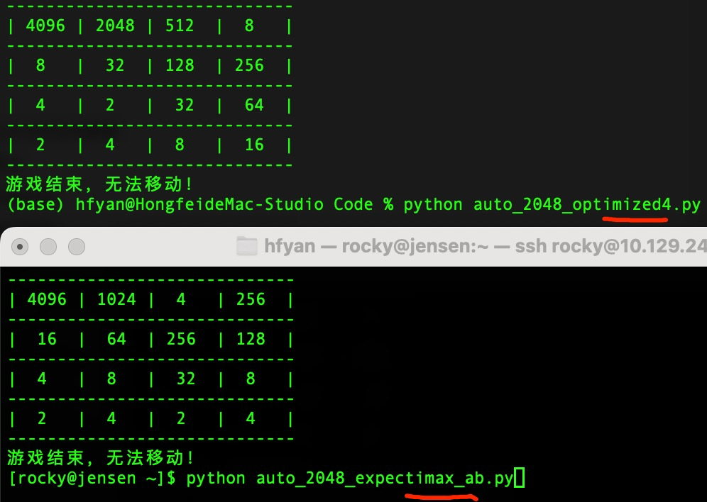 ### Q. vi 里面如何拷贝整个文件?
在Vi或Vim编辑器中,拷贝整个文件的内容可以通过以下步骤实现:
#### 方法一:使用Vim命令
1. 打开你的文件:
```bash
vim yourfile.txt
```
2. 进入命令模式(按 `Esc` 键确保你在命令模式下)。
3. 输入以下命令以选中整个文件的文本:
```
ggVG
```
- `gg` 将光标移动到文件的第一行。
- `V` 进入可视行选择模式。
- `G` 选择从当前行到文件末尾的所有行,组合起来就是全选整个文件。
4. 复制选中的内容(在命令模式下):
```
y
```
这里的 `y` 是 yank 的缩写,用于复制选中的文本。
5. 现在,文件的所有内容已经被复制到了Vim的寄存器中。你可以通过打开另一个文件或者在同一文件中不同的位置粘贴这些内容:
- 打开新文件进行粘贴:
```bash
:e newfile.txt
```
在新文件中,进入插入模式前按 `p` 键粘贴内容。
#### 方法二:直接使用系统剪贴板(如果支持)
如果你的Vim版本支持与系统剪贴板交互,并且你正在使用图形界面版本的Vim(如gvim),可以直接将文件内容发送到系统剪贴板:
1. 在正常模式下输入以下命令来选择并复制整个文件至系统剪贴板:
```
:%y+
```
这里的 `%` 表示整个文件范围,`y+` 表示将选中的内容复制到系统剪贴板。
2. 然后你可以切换到其他应用程序中粘贴这个内容。
请注意,对于方法二,需要确保你的Vim安装了对系统剪贴板的支持(通常需要`+clipboard`特性)。可以通过运行 `vim --version | grep clipboard` 来检查是否支持。如果输出中有 `+clipboard` 则表示支持,如果有 `-clipboard` 则不支持,这种情况下可能需要安装额外的包或使用另一种方法。
### Q.Alpha-Beta剪枝的基本原理
Alpha-Beta剪枝是一种用于博弈树搜索的优化技术,目的是减少评估节点的数量,从而提高Minimax算法的效率。它通过忽略那些不会影响最终决策的部分搜索树来实现这一点。下面是Alpha-Beta剪枝的基本原理的简要说明。
#### 1. 核心概念
不要死记硬背 Alpha 和 Beta,请这样理解:
* **Max(你)**:想要分数越高越好。
* **Min(对手)**:想要分数越低越好。
* **Alpha($\alpha$)**:**你的底线**。意思是“我现在手里已经稳拿 X 分了,更烂的我不要”。
* **Beta($\beta$)**:**对手的底线**(也是你的天花板)。意思是“对手已经能把分压到 Y 分了,如果我这边算出个比 Y 更高的分,对手绝不会让我走这条路”。
#### 2. 树形图表示
假设我们有这样一棵树。
* **第一层(Max)**:轮到你走。
* **第二层(Min)**:轮到对手走。
* **第三层(数字)**:最终的得分。
我们按照**从左到右**的顺序计算。
```text
[Max: 根节点]
/ | \
(A) (B) (C) <-- 对手(Min)层
/ \ / \ / \
3 5 2 ? 9 ?
```
#### 3. 剪枝过程详解(一步步看)
**第一步:探索左边分支 (A)**
1. 电脑先看左边。对手(Min)在 A 节点面临两个选择:3 和 5。
2. 对手很聪明,肯定选小的。所以 **A 节点的价值是 3**。
3. **更新 Alpha(你的底线)**:这时候你(Max)知道了,走左边这一路,**最差也能得 3 分**。
* 当前 **$\alpha = 3$**。
**第二步:探索中间分支 (B) —— 【剪枝发生时刻!】**
1. 电脑开始计算 B 节点。
2. 先看了 B 的第一个子节点:**是 2**。
3. **停!思考一下:**
* 对手(Min)在 B 节点,发现了一个 2。因为对手想要分越低越好,所以不管 B 后面那个问号(?)是多少(哪怕是 0 或 -100),对手在 B 这一路的选择**绝对不会超过 2**。
* 也就是:**B 节点的最终价值 $\le$ 2**。
4. **与你的底线对比**:
* 你(Max)手里已经握着左边的 **3分**(Alpha=3)。
* 而中间这条路(B),对手最仁慈也只会让你得 **2分**。
5. **结论**:你是个正常人,既然左边能得3分,你绝不会选只能得2分的中间这条路。
6. **剪枝**:B 节点后面剩下的那个问号(?),**根本不用算了!** 直接砍掉。
**第三步:探索右边分支 (C)**
1. 电脑开始计算 C 节点。
2. 先看了 C 的第一个子节点:**是 9**。
3. **思考**:
* 对手(Min)在 C 节点看到 9。对手还在找有没有比 9 更小的数。
* 目前 C 的价值 $\le$ 9。
4. **与你的底线对比**:
* 你的底线 Alpha 是 3。
* 目前 C 这条路有可能给你 9 分(如果对手后面没别的招)。
* $9 > 3$,这比你现在的底线好!所以**不能剪枝**,必须继续看 C 后面的问号(?),万一后面是个 1 呢?那对手肯定选 1,你就得不到 9 了。
5. 所以 C 分支必须算完。
#### 总结原理
上面的过程翻译成“剪枝原理”就是:
1. **Alpha 剪枝(发生在 Min 节点,如 B)**:
* 当**对手(Min)** 发现这一步如果走下去,分数比 **你(Max)** 已经拥有的底线(Alpha)还要低。
* **Max 心里话**:“这路太烂了,比我刚才找的路还烂,我不可能走这儿,别算了。” -> **剪掉!**
2. **Beta 剪枝(发生在 Max 节点,反过来)**:
* 当 **你(Max)** 发现这一步如果走下去,分数比 **对手(Min)** 已经设下的限制(Beta)还要高。
* **Min 心里话**:“你想得美!刚才我已经找到让你只能得5分的办法,现在你想走这条得100分的路?我绝不会让你走到这个节点的。” -> **剪掉!**
**记住一句话:**
**剪枝就是因为“已经有一条更好的退路(对 Max 来说)”或者“对手已经抓住了你的把柄(对 Min 来说)”,导致当前的探索变得毫无意义。**
通过这种方式,Alpha-Beta剪枝能够在不改变最终结果的情况下显著减少需要评估的节点数,特别是在理想情况下(比如对手的最佳移动总是最先被考察),它可以将搜索效率提高一倍。
## 3.2 示例:使用预训练模型进行问答。
以Hugging Face Transformer为例,下述 `first_qa.py`代码载入本地中文预训练模型进行问答推理:
> | 模型 | 适用语言 | 用途 |
> | ---------------------------------------- | -------- | -------- |
> | `distilbert-base-cased-distilled-squad` | 英文 | 英文问答 |
> | `uer/roberta-base-chinese-extractive-qa` | 中文 | 中文问答 |
>
> Q: 如何用**浏览器手动下载** `uer/roberta-base-chinese-extractive-qa` 模型,做到完全 **离线部署** 的步骤:
>
> 1. 打开模型页面
>
> 浏览器访问:https://huggingface.co/uer/roberta-base-chinese-extractive-qa
>
> 2. 进入 “Files and versions” 页面,手动下载以下几个关键文件:
>
> | 文件名 | 说明 |
>| ------------------------- | ------------------------------ |
> | `config.json` | 模型结构配置 |
> | `pytorch_model.bin` | 模型权重(很大,400MB 左右) |
> | `tokenizer_config.json` | tokenizer 配置 |
> | `vocab.txt` | 中文词表(必需) |
> | `special_tokens_map.json` | 特殊符号定义(可选但推荐) |
> | `tokenizer.json` | tokenizer 的二进制形式(可选) |
>
> 你可以在网页中依次点击这些文件,然后点击右上角 “Download”。
>
>
>
> 或者这里下载:
>
> https://disk.pku.edu.cn/link/AA5F507BA7BC504334ACA7FCBECFE64995
>Name: model-roberta-chinese-qa.zip
> Expires: Never
> Pickup Code: zXih
我的clab云虚拟机beijing.zhengmao.ltd,`AI_literacy`文件夹
```
[rocky@jensen AI_literacy]$ tree
.
├── first_qa.py
└── models
└── roberta-chinese-qa
├── config.json
├── pytorch_model.bin
├── special_tokens_map.json
├── tokenizer_config.json
└── vocab.txt
```
**创建独立的虚拟环境 & 安装 深度学习框架 PyTorch**
> 为每个项目创建独立的虚拟环境,避免依赖冲突。
>
> ```
> cd ~/AI_literacy # 替换为你的项目路径
> python3 -m venv .venv
> source .venv/bin/activate
> ```
>
> > 退出虚拟环境命令:`deactivate`
>
>
>
> 安装 深度学习框架 PyTorch
> pip install -U transformers
> pip install torch
`first_qa.py`
```python
from transformers import pipeline
qa = pipeline(
"question-answering",
#model="./models/distilbert-base-cased-distilled-squad",
model="./models/roberta-chinese-qa",
tokenizer="./models/roberta-chinese-qa",
framework="pt" # 显式要求使用 PyTorch
)
result = qa(
question="谁是人工智能之父?",
context="艾伦·图灵是人工智能之父,被誉为计算机科学的奠基人。"
)
print(result) # 看完整结果
print(result["answer"]) # 输出应为:艾伦·图灵
```
上述代码中,指定了本地下载的中文问答模型目录,通过pipeline接口直接进行抽取式问答推理。在真实应用中,可替换为更强大的模型(如GPT-4)并结合语言提示(Prompt)实现更复杂的自然语言任务。
运行结果展示
```
(.venv) [rocky@jensen AI_literacy]$ python first_qa.py
Device set to use cpu
{'score': 0.31832563877105713, 'start': 0, 'end': 5, 'answer': '艾伦·图灵'}
艾伦·图灵
```
> 用一个本地的中文问答模型,在一段文本里提取问题的答案。
>
> 1. 引入 Hugging Face 的 `pipeline`
>
> ```python
>from transformers import pipeline
> ```
>
> 这是 Hugging Face `transformers` 提供的简洁 API,用于快速构建 NLP 任务管道,例如文本分类、问答、翻译等。
>
>
>
> 2. 构造问答任务的 pipeline(使用本地模型)
>
> ```python
>qa = pipeline(
> "question-answering",
> #model="./distilbert-base-cased-distilled-squad",
> model="./roberta-chinese-qa", # 使用本地中文模型目录
> framework="pt" # 强制使用 PyTorch
> )
> ```
>
> 参数说明:
>
> | 参数 | 含义 |
>| ------------------------------ | ------------------------------------------------------------ |
> | `"question-answering"` | 指定任务类型是抽取式问答(extractive QA) |
> | `model="./roberta-chinese-qa"` | 指向本地下载的模型文件夹,里面包含 `pytorch_model.bin`、`config.json` 等 |
> | `framework="pt"` | 显式要求使用 PyTorch,而不是 TensorFlow,防止意外加载 TF 模型引发错误 |
>
> `tokenizer` 会自动从模型目录中加载,无需单独指定。
>
> ------
>
> 3. 运行问答推理
>
> ```python
>result = qa(
> question="谁是人工智能之父?",
> context="艾伦·图灵是人工智能之父,被誉为计算机科学的奠基人。"
> )
> ```
>
> 说明:
>
> - 输入的 `question` 是用户要问的问题;
>- `context` 是包含答案的上下文文本(模型会在里面查找答案);
> - 返回的是一个包含 **预测答案位置、内容、置信度** 的字典结构。
>
>
>
> 🛠 常见补充建议:
>
> - **更复杂 context**:你可以给它更多段落,它会找最有可能的答案;
>
> - **中文精度提高**:你可以尝试 `hfl/chinese-roberta-wwm-ext-large` 之类的模型;
>
>
# 4. 神经网络、深度学习和具体应用
如果智能体应该表现得像人类一样,那么它可能需要学习。学习是一种复杂的生物现象,即使是人类自己也没有完全理解。要使人工智能体学习肯定不是件容易的事情。但是在过去已经有好几种方法为未来建立了希望。大多数方法使用了归纳学习或从例子中学习这意味着把很大集合的问题和解法都给计算机,让计算机从中学习。其中一种方法不必使用复杂的数学概念来描述,它就是**神经网络**(neural networks)。神经网络试图使用神经元网络去模仿人脑的学习过程。
图 这一层级关系图展示了不同领域之间的关系。大语言模型是深度学习技术的具体应用,能够处理和生成类似人类语言的文本;深度学习是机器学习的一个分支,主要使用多层神经网络;机器学习和深度学习致力于开发算法,使计算机能够从数据中学习,并执行需要人类智能水平的任务
如图所示,深度学习是机器学习的一个分支,它主要利用3层及以上的神经网络(深度神经网络)来建模数据中的复杂模式和抽象特征。与深度学习不同,传统的机器学习往往需要人工进行特征提取。这意味着人类专家需要为模型识别和挑选出最相关的特征。
尽管人工智能领域现在由机器学习和深度学习所主导,但该领域也涉及其他方法,比如基于规则的系统、遗传算法、专家系统、模糊逻辑或符号推理
**生物神经元**(biological neurons)
人脑中有数以亿计的处理单元,称为**神经元**(neurons)。每个神经元平均与数以千计的其他神经元相连。神经元由三部分构成:胞体(soma)、轴突(axon)和树突(dendrites)。如图所示。
### Q. vi 里面如何拷贝整个文件?
在Vi或Vim编辑器中,拷贝整个文件的内容可以通过以下步骤实现:
#### 方法一:使用Vim命令
1. 打开你的文件:
```bash
vim yourfile.txt
```
2. 进入命令模式(按 `Esc` 键确保你在命令模式下)。
3. 输入以下命令以选中整个文件的文本:
```
ggVG
```
- `gg` 将光标移动到文件的第一行。
- `V` 进入可视行选择模式。
- `G` 选择从当前行到文件末尾的所有行,组合起来就是全选整个文件。
4. 复制选中的内容(在命令模式下):
```
y
```
这里的 `y` 是 yank 的缩写,用于复制选中的文本。
5. 现在,文件的所有内容已经被复制到了Vim的寄存器中。你可以通过打开另一个文件或者在同一文件中不同的位置粘贴这些内容:
- 打开新文件进行粘贴:
```bash
:e newfile.txt
```
在新文件中,进入插入模式前按 `p` 键粘贴内容。
#### 方法二:直接使用系统剪贴板(如果支持)
如果你的Vim版本支持与系统剪贴板交互,并且你正在使用图形界面版本的Vim(如gvim),可以直接将文件内容发送到系统剪贴板:
1. 在正常模式下输入以下命令来选择并复制整个文件至系统剪贴板:
```
:%y+
```
这里的 `%` 表示整个文件范围,`y+` 表示将选中的内容复制到系统剪贴板。
2. 然后你可以切换到其他应用程序中粘贴这个内容。
请注意,对于方法二,需要确保你的Vim安装了对系统剪贴板的支持(通常需要`+clipboard`特性)。可以通过运行 `vim --version | grep clipboard` 来检查是否支持。如果输出中有 `+clipboard` 则表示支持,如果有 `-clipboard` 则不支持,这种情况下可能需要安装额外的包或使用另一种方法。
### Q.Alpha-Beta剪枝的基本原理
Alpha-Beta剪枝是一种用于博弈树搜索的优化技术,目的是减少评估节点的数量,从而提高Minimax算法的效率。它通过忽略那些不会影响最终决策的部分搜索树来实现这一点。下面是Alpha-Beta剪枝的基本原理的简要说明。
#### 1. 核心概念
不要死记硬背 Alpha 和 Beta,请这样理解:
* **Max(你)**:想要分数越高越好。
* **Min(对手)**:想要分数越低越好。
* **Alpha($\alpha$)**:**你的底线**。意思是“我现在手里已经稳拿 X 分了,更烂的我不要”。
* **Beta($\beta$)**:**对手的底线**(也是你的天花板)。意思是“对手已经能把分压到 Y 分了,如果我这边算出个比 Y 更高的分,对手绝不会让我走这条路”。
#### 2. 树形图表示
假设我们有这样一棵树。
* **第一层(Max)**:轮到你走。
* **第二层(Min)**:轮到对手走。
* **第三层(数字)**:最终的得分。
我们按照**从左到右**的顺序计算。
```text
[Max: 根节点]
/ | \
(A) (B) (C) <-- 对手(Min)层
/ \ / \ / \
3 5 2 ? 9 ?
```
#### 3. 剪枝过程详解(一步步看)
**第一步:探索左边分支 (A)**
1. 电脑先看左边。对手(Min)在 A 节点面临两个选择:3 和 5。
2. 对手很聪明,肯定选小的。所以 **A 节点的价值是 3**。
3. **更新 Alpha(你的底线)**:这时候你(Max)知道了,走左边这一路,**最差也能得 3 分**。
* 当前 **$\alpha = 3$**。
**第二步:探索中间分支 (B) —— 【剪枝发生时刻!】**
1. 电脑开始计算 B 节点。
2. 先看了 B 的第一个子节点:**是 2**。
3. **停!思考一下:**
* 对手(Min)在 B 节点,发现了一个 2。因为对手想要分越低越好,所以不管 B 后面那个问号(?)是多少(哪怕是 0 或 -100),对手在 B 这一路的选择**绝对不会超过 2**。
* 也就是:**B 节点的最终价值 $\le$ 2**。
4. **与你的底线对比**:
* 你(Max)手里已经握着左边的 **3分**(Alpha=3)。
* 而中间这条路(B),对手最仁慈也只会让你得 **2分**。
5. **结论**:你是个正常人,既然左边能得3分,你绝不会选只能得2分的中间这条路。
6. **剪枝**:B 节点后面剩下的那个问号(?),**根本不用算了!** 直接砍掉。
**第三步:探索右边分支 (C)**
1. 电脑开始计算 C 节点。
2. 先看了 C 的第一个子节点:**是 9**。
3. **思考**:
* 对手(Min)在 C 节点看到 9。对手还在找有没有比 9 更小的数。
* 目前 C 的价值 $\le$ 9。
4. **与你的底线对比**:
* 你的底线 Alpha 是 3。
* 目前 C 这条路有可能给你 9 分(如果对手后面没别的招)。
* $9 > 3$,这比你现在的底线好!所以**不能剪枝**,必须继续看 C 后面的问号(?),万一后面是个 1 呢?那对手肯定选 1,你就得不到 9 了。
5. 所以 C 分支必须算完。
#### 总结原理
上面的过程翻译成“剪枝原理”就是:
1. **Alpha 剪枝(发生在 Min 节点,如 B)**:
* 当**对手(Min)** 发现这一步如果走下去,分数比 **你(Max)** 已经拥有的底线(Alpha)还要低。
* **Max 心里话**:“这路太烂了,比我刚才找的路还烂,我不可能走这儿,别算了。” -> **剪掉!**
2. **Beta 剪枝(发生在 Max 节点,反过来)**:
* 当 **你(Max)** 发现这一步如果走下去,分数比 **对手(Min)** 已经设下的限制(Beta)还要高。
* **Min 心里话**:“你想得美!刚才我已经找到让你只能得5分的办法,现在你想走这条得100分的路?我绝不会让你走到这个节点的。” -> **剪掉!**
**记住一句话:**
**剪枝就是因为“已经有一条更好的退路(对 Max 来说)”或者“对手已经抓住了你的把柄(对 Min 来说)”,导致当前的探索变得毫无意义。**
通过这种方式,Alpha-Beta剪枝能够在不改变最终结果的情况下显著减少需要评估的节点数,特别是在理想情况下(比如对手的最佳移动总是最先被考察),它可以将搜索效率提高一倍。
## 3.2 示例:使用预训练模型进行问答。
以Hugging Face Transformer为例,下述 `first_qa.py`代码载入本地中文预训练模型进行问答推理:
> | 模型 | 适用语言 | 用途 |
> | ---------------------------------------- | -------- | -------- |
> | `distilbert-base-cased-distilled-squad` | 英文 | 英文问答 |
> | `uer/roberta-base-chinese-extractive-qa` | 中文 | 中文问答 |
>
> Q: 如何用**浏览器手动下载** `uer/roberta-base-chinese-extractive-qa` 模型,做到完全 **离线部署** 的步骤:
>
> 1. 打开模型页面
>
> 浏览器访问:https://huggingface.co/uer/roberta-base-chinese-extractive-qa
>
> 2. 进入 “Files and versions” 页面,手动下载以下几个关键文件:
>
> | 文件名 | 说明 |
>| ------------------------- | ------------------------------ |
> | `config.json` | 模型结构配置 |
> | `pytorch_model.bin` | 模型权重(很大,400MB 左右) |
> | `tokenizer_config.json` | tokenizer 配置 |
> | `vocab.txt` | 中文词表(必需) |
> | `special_tokens_map.json` | 特殊符号定义(可选但推荐) |
> | `tokenizer.json` | tokenizer 的二进制形式(可选) |
>
> 你可以在网页中依次点击这些文件,然后点击右上角 “Download”。
>
>
>
> 或者这里下载:
>
> https://disk.pku.edu.cn/link/AA5F507BA7BC504334ACA7FCBECFE64995
>Name: model-roberta-chinese-qa.zip
> Expires: Never
> Pickup Code: zXih
我的clab云虚拟机beijing.zhengmao.ltd,`AI_literacy`文件夹
```
[rocky@jensen AI_literacy]$ tree
.
├── first_qa.py
└── models
└── roberta-chinese-qa
├── config.json
├── pytorch_model.bin
├── special_tokens_map.json
├── tokenizer_config.json
└── vocab.txt
```
**创建独立的虚拟环境 & 安装 深度学习框架 PyTorch**
> 为每个项目创建独立的虚拟环境,避免依赖冲突。
>
> ```
> cd ~/AI_literacy # 替换为你的项目路径
> python3 -m venv .venv
> source .venv/bin/activate
> ```
>
> > 退出虚拟环境命令:`deactivate`
>
>
>
> 安装 深度学习框架 PyTorch
> pip install -U transformers
> pip install torch
`first_qa.py`
```python
from transformers import pipeline
qa = pipeline(
"question-answering",
#model="./models/distilbert-base-cased-distilled-squad",
model="./models/roberta-chinese-qa",
tokenizer="./models/roberta-chinese-qa",
framework="pt" # 显式要求使用 PyTorch
)
result = qa(
question="谁是人工智能之父?",
context="艾伦·图灵是人工智能之父,被誉为计算机科学的奠基人。"
)
print(result) # 看完整结果
print(result["answer"]) # 输出应为:艾伦·图灵
```
上述代码中,指定了本地下载的中文问答模型目录,通过pipeline接口直接进行抽取式问答推理。在真实应用中,可替换为更强大的模型(如GPT-4)并结合语言提示(Prompt)实现更复杂的自然语言任务。
运行结果展示
```
(.venv) [rocky@jensen AI_literacy]$ python first_qa.py
Device set to use cpu
{'score': 0.31832563877105713, 'start': 0, 'end': 5, 'answer': '艾伦·图灵'}
艾伦·图灵
```
> 用一个本地的中文问答模型,在一段文本里提取问题的答案。
>
> 1. 引入 Hugging Face 的 `pipeline`
>
> ```python
>from transformers import pipeline
> ```
>
> 这是 Hugging Face `transformers` 提供的简洁 API,用于快速构建 NLP 任务管道,例如文本分类、问答、翻译等。
>
>
>
> 2. 构造问答任务的 pipeline(使用本地模型)
>
> ```python
>qa = pipeline(
> "question-answering",
> #model="./distilbert-base-cased-distilled-squad",
> model="./roberta-chinese-qa", # 使用本地中文模型目录
> framework="pt" # 强制使用 PyTorch
> )
> ```
>
> 参数说明:
>
> | 参数 | 含义 |
>| ------------------------------ | ------------------------------------------------------------ |
> | `"question-answering"` | 指定任务类型是抽取式问答(extractive QA) |
> | `model="./roberta-chinese-qa"` | 指向本地下载的模型文件夹,里面包含 `pytorch_model.bin`、`config.json` 等 |
> | `framework="pt"` | 显式要求使用 PyTorch,而不是 TensorFlow,防止意外加载 TF 模型引发错误 |
>
> `tokenizer` 会自动从模型目录中加载,无需单独指定。
>
> ------
>
> 3. 运行问答推理
>
> ```python
>result = qa(
> question="谁是人工智能之父?",
> context="艾伦·图灵是人工智能之父,被誉为计算机科学的奠基人。"
> )
> ```
>
> 说明:
>
> - 输入的 `question` 是用户要问的问题;
>- `context` 是包含答案的上下文文本(模型会在里面查找答案);
> - 返回的是一个包含 **预测答案位置、内容、置信度** 的字典结构。
>
>
>
> 🛠 常见补充建议:
>
> - **更复杂 context**:你可以给它更多段落,它会找最有可能的答案;
>
> - **中文精度提高**:你可以尝试 `hfl/chinese-roberta-wwm-ext-large` 之类的模型;
>
>
# 4. 神经网络、深度学习和具体应用
如果智能体应该表现得像人类一样,那么它可能需要学习。学习是一种复杂的生物现象,即使是人类自己也没有完全理解。要使人工智能体学习肯定不是件容易的事情。但是在过去已经有好几种方法为未来建立了希望。大多数方法使用了归纳学习或从例子中学习这意味着把很大集合的问题和解法都给计算机,让计算机从中学习。其中一种方法不必使用复杂的数学概念来描述,它就是**神经网络**(neural networks)。神经网络试图使用神经元网络去模仿人脑的学习过程。

图 这一层级关系图展示了不同领域之间的关系。大语言模型是深度学习技术的具体应用,能够处理和生成类似人类语言的文本;深度学习是机器学习的一个分支,主要使用多层神经网络;机器学习和深度学习致力于开发算法,使计算机能够从数据中学习,并执行需要人类智能水平的任务
如图所示,深度学习是机器学习的一个分支,它主要利用3层及以上的神经网络(深度神经网络)来建模数据中的复杂模式和抽象特征。与深度学习不同,传统的机器学习往往需要人工进行特征提取。这意味着人类专家需要为模型识别和挑选出最相关的特征。
尽管人工智能领域现在由机器学习和深度学习所主导,但该领域也涉及其他方法,比如基于规则的系统、遗传算法、专家系统、模糊逻辑或符号推理
**生物神经元**(biological neurons)
人脑中有数以亿计的处理单元,称为**神经元**(neurons)。每个神经元平均与数以千计的其他神经元相连。神经元由三部分构成:胞体(soma)、轴突(axon)和树突(dendrites)。如图所示。
 >
> **输入**
>
> 输入共四行。
>
> \- 第一行包含三个整数 N, L, M,分别表示每层的城市数量、层数,以及所需整除的代价模数。
> \- 第二行包含 N 个整数,表示从入口点到第 1 层每个城市的代价。
> \- 第三行包含 N 个整数,表示任意相邻层之间的代价数组 c_1, c_2, ..., c_N,其中 c_j 表示连接至每层中第 j 个城市的代价。
> \- 第四行包含 N 个整数,表示从第 L 层的每个城市到出口的代价。
>
> 1 <= N <= 10^6
>
> 2 <= L <= 10^5
>
> 2 <= M <= 100
>
> 0 <= cost <= M
>
> **输出**
>
> 输出一个整数,表示从入口到出口总代价可以被 M 整除的路径条数,结果对 10^9 + 7 取模。
>
> 样例输入
>
> ```
> 2 3 13
> 4 6
> 2 1
> 3 4
> ```
>
> 样例输出
>
> ```
> 2
> ```
>
> 提示
>
> 动态规划
>
> 该国家结构如下,共有 3 层,每层有 2 个城市:
>
> \- 入口到第一层城市的代价分别为 4 和 6。
> \- 每对相邻层之间,连接至第一个城市的代价为 2,至第二个城市的代价为 1。
> \- 最后一层到出口的代价分别为 3 和 4。
>
> 共计有 N^L = 2^3 = 8 条路径。仅有两条路径的总代价可被 13 整除。
>
> 来源
>
> TA-xjk
> ## M29740:神经网络
>
> 拓扑排序, AI, http://cs101.openjudge.cn/2025springcs201testing/M29740/
>
> 随着深度学习技术的发展,神经网络已广泛应用于图像识别、自然语言处理、推荐系统等多个领域。近年来,图神经网络(Graph Neural Networks, GNN)作为一种能够处理非欧式结构化数据的深度学习方法,越来越受到研究者关注。小P同学最近在学习图神经网络的基础知识时,尝试设计了一个简化的“前馈图神经网络”模型,并希望借助编程来验证其推理过程是否合理。
>
> 在小P的模型中,一个图神经网络被抽象成一个**有向图**,图中的节点代表神经元(或计算单元),边则表示信息的传递通道。任意两个节点之间逻辑上至多视为一条有向边。下图是一个神经元节点的示意图:
>
>
>
> **输入**
>
> 输入共四行。
>
> \- 第一行包含三个整数 N, L, M,分别表示每层的城市数量、层数,以及所需整除的代价模数。
> \- 第二行包含 N 个整数,表示从入口点到第 1 层每个城市的代价。
> \- 第三行包含 N 个整数,表示任意相邻层之间的代价数组 c_1, c_2, ..., c_N,其中 c_j 表示连接至每层中第 j 个城市的代价。
> \- 第四行包含 N 个整数,表示从第 L 层的每个城市到出口的代价。
>
> 1 <= N <= 10^6
>
> 2 <= L <= 10^5
>
> 2 <= M <= 100
>
> 0 <= cost <= M
>
> **输出**
>
> 输出一个整数,表示从入口到出口总代价可以被 M 整除的路径条数,结果对 10^9 + 7 取模。
>
> 样例输入
>
> ```
> 2 3 13
> 4 6
> 2 1
> 3 4
> ```
>
> 样例输出
>
> ```
> 2
> ```
>
> 提示
>
> 动态规划
>
> 该国家结构如下,共有 3 层,每层有 2 个城市:
>
> \- 入口到第一层城市的代价分别为 4 和 6。
> \- 每对相邻层之间,连接至第一个城市的代价为 2,至第二个城市的代价为 1。
> \- 最后一层到出口的代价分别为 3 和 4。
>
> 共计有 N^L = 2^3 = 8 条路径。仅有两条路径的总代价可被 13 整除。
>
> 来源
>
> TA-xjk
> ## M29740:神经网络
>
> 拓扑排序, AI, http://cs101.openjudge.cn/2025springcs201testing/M29740/
>
> 随着深度学习技术的发展,神经网络已广泛应用于图像识别、自然语言处理、推荐系统等多个领域。近年来,图神经网络(Graph Neural Networks, GNN)作为一种能够处理非欧式结构化数据的深度学习方法,越来越受到研究者关注。小P同学最近在学习图神经网络的基础知识时,尝试设计了一个简化的“前馈图神经网络”模型,并希望借助编程来验证其推理过程是否合理。
>
> 在小P的模型中,一个图神经网络被抽象成一个**有向图**,图中的节点代表神经元(或计算单元),边则表示信息的传递通道。任意两个节点之间逻辑上至多视为一条有向边。下图是一个神经元节点的示意图:
>
>  >
> 神经元(编号为 i)
>
> 图中,X1 ~ X3 表示来自上游节点的信息输入,Y1 ~ Y2 是向下游节点的输出通道,Ci 表示神经元当前的激活值(activation),而 Ui 是该节点的偏置项(bias),可视为其内在的阈值参数。
>
> 神经元按一定的顺序排列,构成整个图神经网络。在小P的模型之中,神经元近似于分层摆放,可以近似视作输入层、若干隐藏层与输出层;信息只能沿有向边由前向后传播。下图是一个最简单的三层神经网络的例子。
>
>
>
> 神经元(编号为 i)
>
> 图中,X1 ~ X3 表示来自上游节点的信息输入,Y1 ~ Y2 是向下游节点的输出通道,Ci 表示神经元当前的激活值(activation),而 Ui 是该节点的偏置项(bias),可视为其内在的阈值参数。
>
> 神经元按一定的顺序排列,构成整个图神经网络。在小P的模型之中,神经元近似于分层摆放,可以近似视作输入层、若干隐藏层与输出层;信息只能沿有向边由前向后传播。下图是一个最简单的三层神经网络的例子。
>
>  >
> > 现实中若某些突触损坏,会产生“闭环反馈”使整个网络失效。若这幅有向图 **存在回路(哪怕仅为自环)**,称为**神经坏死**,网络将彻底无法工作。
>
> 小P定义的神经元更新规则如下(令 n 表示总神经元数量):
>
>
>
> > 现实中若某些突触损坏,会产生“闭环反馈”使整个网络失效。若这幅有向图 **存在回路(哪怕仅为自环)**,称为**神经坏死**,网络将彻底无法工作。
>
> 小P定义的神经元更新规则如下(令 n 表示总神经元数量):
>
>  >
> 其中:
>
> - Wji 表示从节点 j 到节点 i 的边权重(可以为负值)
> - Cj 是上游神经元的当前激活值
> - Ui 是当前神经元的偏置项
> - 若 Ci > 0,则该神经元处于激活(active)状态,下一时刻将以强度Ci 向下一层传递信号;否则,它将保持静默(inactive)
>
> 当输入层(入度为0的节点)的神经元激活后,该网络模型将以类似于图神经网络的方式逐层传播信号,最终在输出层(出度为0的节点)产生结果。
>
> 输入
>
> 输入文件第一行是两个整数 n(1≤n≤100)和 p(0 ≤ p ≤ n(n-1))。
>
> 接下来 n 行,每行 2 个整数,第 i+1 行是神经元 i 最初状态和其阈值(Ui),非输入层的神经元开始时状态必然为 0。
>
> 再下面 p 行,每行有两个整数 i,j 及一个整数 Wij,表示连接神经元 i,j 的边权值为 Wij。(i,j) 二元组可重复出现,若重复则视作一条边,将权重累加即可。
>
> 输出
>
> 输出文件包含若干行,每行有 2 个整数,分别对应一个神经元的编号,及其最后的状态,2 个整数间以空格分隔。仅输出最后状态大于 0 的输出层神经元状态,并且按照编号由小到大顺序输出。
>
> 若图中存在任何有向环(神经坏死),或所有输出层神经元最后状态均 ≤0,则输出 NULL。
>
> 样例输入
>
> ```
> 样例1:
> 5 6
> 1 0
> 1 0
> 0 1
> 0 1
> 0 1
> 1 3 1
> 1 4 1
> 1 5 1
> 2 3 1
> 2 4 1
> 2 5 1
>
> 样例2:
> 2 2
> 1 0
> 0 0
> 1 2 1
> 2 1 1
> ```
>
> 样例输出
>
> ```
> 样例1:
> 3 1
> 4 1
> 5 1
>
> 样例2:
> NULL
> ```
>
> 提示
>
> 拓扑排序,AI
>
> 输入层神经元状态不需减去其偏置项
> 输入层可以激活也可以不激活,C <= 0 是不激活输入层
>
> C/C++,变量类型需要考虑long long以防止溢出
>
> 来源
>
> TA-xjk
深度学习是连接主义流派的核心方法之一,其核心思想是利用**多层神经网络**自动从数据中学习层次化的特征表示。本节将系统介绍神经网络的关键训练机制——**反向传播算法**,并结合5个由浅入深的应用示例,帮助读者掌握从基础建模到复杂图像分类任务的完整流程。
**反向传播**(Backpropagation)
**反向传播** 是训练神经网络的基石算法。它通过两个阶段协同工作:
1. **前向传播**:输入数据逐层经过加权求和与非线性激活函数(如 ReLU、Softmax),最终输出预测结果;
2. **反向传播**:基于损失函数(如交叉熵、均方误差)计算预测值与真实标签之间的误差,并利用**链式法则**高效地计算损失对每一层参数的梯度。
随后,优化器(如 SGD、Adam)依据这些梯度更新网络权重,目标是最小化整体损失。这一机制使得训练包含数十甚至上百层的深度网络成为可能,直接推动了深度学习的爆发式发展。
**反向传播算法流程**
1. **前向传播**:输入 → 逐层计算 → 输出预测值 $\hat{y}$
2. **损失计算**:$L = \text{Loss}(\hat{y}, y)$
3. **梯度反传**:从输出层向输入层,逐层计算 $\frac{\partial L}{\partial w}$ 和 $\frac{\partial L}{\partial b}$
4. **参数更新**:例如使用梯度下降:
$$ w \leftarrow w - \eta \cdot \frac{\partial L}{\partial w} $$
其中 $\eta$ 为学习率。
5. **迭代训练**:遍历训练集多个 epoch,直至损失收敛或达到预设轮次。
> **只要你按梯度的反方向走,数学保证你的 $L$ 一定会减小(只要步长 $\eta$ 别太大)。**
>
> 一次迭代变化量是 **学习率 $\times$ 梯度**($\eta \cdot \frac{\partial L}{\partial w}$)。
>
> * **前向传播**算出你在多高 ($L$)。
>
> * **反向传播**算出你脚下的坡度 ($\frac{\partial L}{\partial w}$)。物理意义是:“当你改变一点点 `w` 时,`L` 变化得有多快(以及往哪个方向变)。”
>
> * **参数更新**决定你往下跳多远 ($\Delta w = -\eta \cdot \text{梯度}$)。
>
>
>
> $$ \Delta w = - \eta \times \frac{\partial L}{\partial w} $$
> 其中:
>
> * $\Delta w$:参数的变化量(这一步走多远)。
> * $\eta$(Eta):**学习率**(是一个预设的常数,比如 0.01),而不是损失值 $L$。
> * $\frac{\partial L}{\partial w}$:**梯度/偏导数**(告诉我们哪个方向下降最快,以及有多陡)。
>
> **Q:如何直观理解这三个物理量?**
>
> 为了理解“单位时间变化”,可以用**“下山”**的物理模型来类比:
>
> * **$L$ (Loss / 损失)**:代表你当前所在的**海拔高度**。
> * *目标*:走到海拔最低的山谷。
> * **$w$ (Weight / 参数)**:代表你所在的**地图坐标**(经纬度)。
> * **$\frac{\partial L}{\partial w}$ (Gradient / 梯度)**:代表你脚下地面的**坡度(倾斜程度)**。
> * 如果坡度很大,说明这里很陡;如果坡度为0,说明是平地。
> * **$\eta$ (Learning Rate / 学习率)**:代表你的**步长**(或者可以说是你跨出一步的时间跨度)。
>
> **现在的逻辑是:**你需要用**“步长($\eta$)”**乘以**“坡度(梯度)”**,来决定你下一步往那个方向迈多大。
>
> **Q:为什么是“学习率 $\times$ 偏导”?**
>
> 在微积分中:
>
> 1. **导数(偏导)的物理意义是“速度”或“趋势”**:
> $\frac{\partial L}{\partial w}$ 告诉我们在当前点,如果我们稍微改变一点点 $w$,$L$ 会变化多快。
>
> 2. **更新公式的本质**:
> 我们希望 $w$ 往 $L$ 减小的方向移动。
> $$ w_{new} = w_{old} - \text{步长} \times \text{坡度} $$
> * 如果**坡度很大**(梯度大),说明离谷底还远或者地形很陡,我们通常会走得比较急(变化量大)。
> * 如果**坡度很小**(梯度接近0),说明快到谷底了,我们会慢慢走(变化量小),以免走过头。
> * **学习率 $\eta$** 起到了调节器的作用。
>
>
> ⚠️ **注意**:深层网络易遭遇**梯度消失**(vanishing gradients)或**梯度爆炸**(exploding gradients)问题,尤其在使用 Sigmoid 或 Tanh 激活函数时。现代实践中常采用 **ReLU 激活函数**、**批归一化(BatchNorm)** 和**残差连接(ResNet)** 等技术加以缓解。
**交互可视化:理解神经网络**
Google 提供了一个优秀的交互式神经网络训练工具,帮助直观理解模型如何分离非线性可分数据:
https://developers.google.com/machine-learning/crash-course/neural-networks/interactive-exercises?hl=zh-cn
**任务目标**:配置一个神经网络,使其能够将下图中的橙点与蓝点分开,并在训练数据和测试数据上实现低于 0.2 的损失。
**操作指南:**
1. 调整网络结构:
- 点击 **HIDDEN LAYERS** 左侧的 **+ / –** 添加/删除隐藏层;
- 点击某隐藏层上方的 **+ / –** 调整该层神经元数量。
2. 修改超参数:
- 从 **Learning rate** 下拉菜单选择合适的学习率(建议尝试 0.01 ~ 0.1);
- 从 **Activation** 下拉菜单选择激活函数(推荐 **ReLU**)。
3. 点击 ▶️ 开始训练,观察损失曲线与决策边界演化。
4. 若未达标,点击 **Reset** 并尝试新配置。
**成功示例截图如下**(损失均低于 0.2):
>
> 其中:
>
> - Wji 表示从节点 j 到节点 i 的边权重(可以为负值)
> - Cj 是上游神经元的当前激活值
> - Ui 是当前神经元的偏置项
> - 若 Ci > 0,则该神经元处于激活(active)状态,下一时刻将以强度Ci 向下一层传递信号;否则,它将保持静默(inactive)
>
> 当输入层(入度为0的节点)的神经元激活后,该网络模型将以类似于图神经网络的方式逐层传播信号,最终在输出层(出度为0的节点)产生结果。
>
> 输入
>
> 输入文件第一行是两个整数 n(1≤n≤100)和 p(0 ≤ p ≤ n(n-1))。
>
> 接下来 n 行,每行 2 个整数,第 i+1 行是神经元 i 最初状态和其阈值(Ui),非输入层的神经元开始时状态必然为 0。
>
> 再下面 p 行,每行有两个整数 i,j 及一个整数 Wij,表示连接神经元 i,j 的边权值为 Wij。(i,j) 二元组可重复出现,若重复则视作一条边,将权重累加即可。
>
> 输出
>
> 输出文件包含若干行,每行有 2 个整数,分别对应一个神经元的编号,及其最后的状态,2 个整数间以空格分隔。仅输出最后状态大于 0 的输出层神经元状态,并且按照编号由小到大顺序输出。
>
> 若图中存在任何有向环(神经坏死),或所有输出层神经元最后状态均 ≤0,则输出 NULL。
>
> 样例输入
>
> ```
> 样例1:
> 5 6
> 1 0
> 1 0
> 0 1
> 0 1
> 0 1
> 1 3 1
> 1 4 1
> 1 5 1
> 2 3 1
> 2 4 1
> 2 5 1
>
> 样例2:
> 2 2
> 1 0
> 0 0
> 1 2 1
> 2 1 1
> ```
>
> 样例输出
>
> ```
> 样例1:
> 3 1
> 4 1
> 5 1
>
> 样例2:
> NULL
> ```
>
> 提示
>
> 拓扑排序,AI
>
> 输入层神经元状态不需减去其偏置项
> 输入层可以激活也可以不激活,C <= 0 是不激活输入层
>
> C/C++,变量类型需要考虑long long以防止溢出
>
> 来源
>
> TA-xjk
深度学习是连接主义流派的核心方法之一,其核心思想是利用**多层神经网络**自动从数据中学习层次化的特征表示。本节将系统介绍神经网络的关键训练机制——**反向传播算法**,并结合5个由浅入深的应用示例,帮助读者掌握从基础建模到复杂图像分类任务的完整流程。
**反向传播**(Backpropagation)
**反向传播** 是训练神经网络的基石算法。它通过两个阶段协同工作:
1. **前向传播**:输入数据逐层经过加权求和与非线性激活函数(如 ReLU、Softmax),最终输出预测结果;
2. **反向传播**:基于损失函数(如交叉熵、均方误差)计算预测值与真实标签之间的误差,并利用**链式法则**高效地计算损失对每一层参数的梯度。
随后,优化器(如 SGD、Adam)依据这些梯度更新网络权重,目标是最小化整体损失。这一机制使得训练包含数十甚至上百层的深度网络成为可能,直接推动了深度学习的爆发式发展。
**反向传播算法流程**
1. **前向传播**:输入 → 逐层计算 → 输出预测值 $\hat{y}$
2. **损失计算**:$L = \text{Loss}(\hat{y}, y)$
3. **梯度反传**:从输出层向输入层,逐层计算 $\frac{\partial L}{\partial w}$ 和 $\frac{\partial L}{\partial b}$
4. **参数更新**:例如使用梯度下降:
$$ w \leftarrow w - \eta \cdot \frac{\partial L}{\partial w} $$
其中 $\eta$ 为学习率。
5. **迭代训练**:遍历训练集多个 epoch,直至损失收敛或达到预设轮次。
> **只要你按梯度的反方向走,数学保证你的 $L$ 一定会减小(只要步长 $\eta$ 别太大)。**
>
> 一次迭代变化量是 **学习率 $\times$ 梯度**($\eta \cdot \frac{\partial L}{\partial w}$)。
>
> * **前向传播**算出你在多高 ($L$)。
>
> * **反向传播**算出你脚下的坡度 ($\frac{\partial L}{\partial w}$)。物理意义是:“当你改变一点点 `w` 时,`L` 变化得有多快(以及往哪个方向变)。”
>
> * **参数更新**决定你往下跳多远 ($\Delta w = -\eta \cdot \text{梯度}$)。
>
>
>
> $$ \Delta w = - \eta \times \frac{\partial L}{\partial w} $$
> 其中:
>
> * $\Delta w$:参数的变化量(这一步走多远)。
> * $\eta$(Eta):**学习率**(是一个预设的常数,比如 0.01),而不是损失值 $L$。
> * $\frac{\partial L}{\partial w}$:**梯度/偏导数**(告诉我们哪个方向下降最快,以及有多陡)。
>
> **Q:如何直观理解这三个物理量?**
>
> 为了理解“单位时间变化”,可以用**“下山”**的物理模型来类比:
>
> * **$L$ (Loss / 损失)**:代表你当前所在的**海拔高度**。
> * *目标*:走到海拔最低的山谷。
> * **$w$ (Weight / 参数)**:代表你所在的**地图坐标**(经纬度)。
> * **$\frac{\partial L}{\partial w}$ (Gradient / 梯度)**:代表你脚下地面的**坡度(倾斜程度)**。
> * 如果坡度很大,说明这里很陡;如果坡度为0,说明是平地。
> * **$\eta$ (Learning Rate / 学习率)**:代表你的**步长**(或者可以说是你跨出一步的时间跨度)。
>
> **现在的逻辑是:**你需要用**“步长($\eta$)”**乘以**“坡度(梯度)”**,来决定你下一步往那个方向迈多大。
>
> **Q:为什么是“学习率 $\times$ 偏导”?**
>
> 在微积分中:
>
> 1. **导数(偏导)的物理意义是“速度”或“趋势”**:
> $\frac{\partial L}{\partial w}$ 告诉我们在当前点,如果我们稍微改变一点点 $w$,$L$ 会变化多快。
>
> 2. **更新公式的本质**:
> 我们希望 $w$ 往 $L$ 减小的方向移动。
> $$ w_{new} = w_{old} - \text{步长} \times \text{坡度} $$
> * 如果**坡度很大**(梯度大),说明离谷底还远或者地形很陡,我们通常会走得比较急(变化量大)。
> * 如果**坡度很小**(梯度接近0),说明快到谷底了,我们会慢慢走(变化量小),以免走过头。
> * **学习率 $\eta$** 起到了调节器的作用。
>
>
> ⚠️ **注意**:深层网络易遭遇**梯度消失**(vanishing gradients)或**梯度爆炸**(exploding gradients)问题,尤其在使用 Sigmoid 或 Tanh 激活函数时。现代实践中常采用 **ReLU 激活函数**、**批归一化(BatchNorm)** 和**残差连接(ResNet)** 等技术加以缓解。
**交互可视化:理解神经网络**
Google 提供了一个优秀的交互式神经网络训练工具,帮助直观理解模型如何分离非线性可分数据:
https://developers.google.com/machine-learning/crash-course/neural-networks/interactive-exercises?hl=zh-cn
**任务目标**:配置一个神经网络,使其能够将下图中的橙点与蓝点分开,并在训练数据和测试数据上实现低于 0.2 的损失。
**操作指南:**
1. 调整网络结构:
- 点击 **HIDDEN LAYERS** 左侧的 **+ / –** 添加/删除隐藏层;
- 点击某隐藏层上方的 **+ / –** 调整该层神经元数量。
2. 修改超参数:
- 从 **Learning rate** 下拉菜单选择合适的学习率(建议尝试 0.01 ~ 0.1);
- 从 **Activation** 下拉菜单选择激活函数(推荐 **ReLU**)。
3. 点击 ▶️ 开始训练,观察损失曲线与决策边界演化。
4. 若未达标,点击 **Reset** 并尝试新配置。
**成功示例截图如下**(损失均低于 0.2):
 **PyTorch 实战:5 个神经网络应用示例**
以下示例涵盖从手动实现到现代架构的完整演进路径。后四个示例使用PyTorch编写, 教程在 https://www.runoob.com/pytorch/pytorch-tutorial.html 或参看附录 A。
| 编号 | 示例名称 | 内容概述 | 技术要点 |
| ---- | ---------------------------- | ------------------------------------------------- | ------------------------------------------ |
| 1 | `0_xor_bp_neural_net_manual` | 手动实现反向传播,解决 XOR 非线性分类问题 | 张量运算、梯度手动计算、无框架依赖 |
| 2 | `1_iris_neural_network` | 使用全连接网络对鸢尾花数据集进行三分类 | 数据加载、`nn.Module`、交叉熵损失 |
| 3 | `2_mnist_resnet18` | 微调 ResNet18 对 MNIST 手写数字分类 | 迁移学习、图像预处理、`torchvision.models` |
| 4 | `3_cifar10_resnet18` | 在 CIFAR-10 上训练 ResNet18 | 数据增强、学习率调度、GPU 加速 |
| 5 | `4_tiny_imagenet_resnet50` | 使用 ResNet50 处理更复杂的 Tiny ImageNet 分类任务 | 大规模数据处理、模型微调、性能评估 |
> 所有代码均可在配套仓库(https://github.com/GMyhf/2025spring-cs201/tree/main/LLM)中找到,建议按顺序实践,逐步掌握从“理解原理”到“工程部署”的完整技能链。
## 4.1 在异或问题(XOR)中手动实现反向传播
异或问题是经典的非线性可分问题,用来演示神经网络的学习能力。一个简单的神经网络可手动实现反向传播来解决异或。以下先给出简洁的伪代码,再给出可以运行的Python代码示例展示了反向传播更新权重的方式:
```python
# 假设网络结构:输入层2个节点,隐藏层2个节点,输出层1个节点
# 初始化权重
W1 = random([...]) # 输入到隐藏层
W2 = random([...]) # 隐藏层到输出层
learning_rate = 0.1
for epoch in range(epochs):
# 前向计算
hidden = sigmoid(X @ W1) # X为输入[四组XOR输入]
output = sigmoid(hidden @ W2) # 预测
# 计算误差
error = (y - output) # y为真实标签
# 反向传播(链式法则)
dW2 = hidden.T @ (error * output * (1 - output))
dW1 = X.T @ ((error * output * (1 - output)) @ W2.T * hidden * (1 - hidden))
# 更新权重
W2 += learning_rate * dW2
W1 += learning_rate * dW1
```
Backpropagation in Neural Network
https://www.geeksforgeeks.org/machine-learning/backpropagation-in-neural-network/
反向传播(Back Propagation),又称为“误差的反向传播”,是一种用于训练神经网络的方法。其目标是通过调整网络中的权重(weights)和偏置(biases),来减小模型预测输出与实际输出之间的差异。
它通过迭代方式更新权重和偏置,以最小化损失函数(cost function)。在每一个训练周期(epoch)中,模型会根据误差梯度(error gradient)更新参数,常用的优化算法包括梯度下降(Gradient Descent)或随机梯度下降(SGD)。该算法使用微积分中的链式法则来计算梯度,从而能够有效地穿越复杂的神经网络结构,优化损失函数。
> Back Propagation is also known as "Backward Propagation of Errors" is a method used to train neural network . Its goal is to reduce the difference between the model’s predicted output and the actual output by adjusting the weights and biases in the network.
>
> It works iteratively to adjust weights and bias to minimize the cost function. In each epoch the model adapts these parameters by reducing loss by following the error gradient. It often uses optimization algorithms like **gradient descent** or **stochastic gradient descent**. The algorithm computes the gradient using the chain rule from calculus allowing it to effectively navigate complex layers in the neural network to minimize the cost function.
**PyTorch 实战:5 个神经网络应用示例**
以下示例涵盖从手动实现到现代架构的完整演进路径。后四个示例使用PyTorch编写, 教程在 https://www.runoob.com/pytorch/pytorch-tutorial.html 或参看附录 A。
| 编号 | 示例名称 | 内容概述 | 技术要点 |
| ---- | ---------------------------- | ------------------------------------------------- | ------------------------------------------ |
| 1 | `0_xor_bp_neural_net_manual` | 手动实现反向传播,解决 XOR 非线性分类问题 | 张量运算、梯度手动计算、无框架依赖 |
| 2 | `1_iris_neural_network` | 使用全连接网络对鸢尾花数据集进行三分类 | 数据加载、`nn.Module`、交叉熵损失 |
| 3 | `2_mnist_resnet18` | 微调 ResNet18 对 MNIST 手写数字分类 | 迁移学习、图像预处理、`torchvision.models` |
| 4 | `3_cifar10_resnet18` | 在 CIFAR-10 上训练 ResNet18 | 数据增强、学习率调度、GPU 加速 |
| 5 | `4_tiny_imagenet_resnet50` | 使用 ResNet50 处理更复杂的 Tiny ImageNet 分类任务 | 大规模数据处理、模型微调、性能评估 |
> 所有代码均可在配套仓库(https://github.com/GMyhf/2025spring-cs201/tree/main/LLM)中找到,建议按顺序实践,逐步掌握从“理解原理”到“工程部署”的完整技能链。
## 4.1 在异或问题(XOR)中手动实现反向传播
异或问题是经典的非线性可分问题,用来演示神经网络的学习能力。一个简单的神经网络可手动实现反向传播来解决异或。以下先给出简洁的伪代码,再给出可以运行的Python代码示例展示了反向传播更新权重的方式:
```python
# 假设网络结构:输入层2个节点,隐藏层2个节点,输出层1个节点
# 初始化权重
W1 = random([...]) # 输入到隐藏层
W2 = random([...]) # 隐藏层到输出层
learning_rate = 0.1
for epoch in range(epochs):
# 前向计算
hidden = sigmoid(X @ W1) # X为输入[四组XOR输入]
output = sigmoid(hidden @ W2) # 预测
# 计算误差
error = (y - output) # y为真实标签
# 反向传播(链式法则)
dW2 = hidden.T @ (error * output * (1 - output))
dW1 = X.T @ ((error * output * (1 - output)) @ W2.T * hidden * (1 - hidden))
# 更新权重
W2 += learning_rate * dW2
W1 += learning_rate * dW1
```
Backpropagation in Neural Network
https://www.geeksforgeeks.org/machine-learning/backpropagation-in-neural-network/
反向传播(Back Propagation),又称为“误差的反向传播”,是一种用于训练神经网络的方法。其目标是通过调整网络中的权重(weights)和偏置(biases),来减小模型预测输出与实际输出之间的差异。
它通过迭代方式更新权重和偏置,以最小化损失函数(cost function)。在每一个训练周期(epoch)中,模型会根据误差梯度(error gradient)更新参数,常用的优化算法包括梯度下降(Gradient Descent)或随机梯度下降(SGD)。该算法使用微积分中的链式法则来计算梯度,从而能够有效地穿越复杂的神经网络结构,优化损失函数。
> Back Propagation is also known as "Backward Propagation of Errors" is a method used to train neural network . Its goal is to reduce the difference between the model’s predicted output and the actual output by adjusting the weights and biases in the network.
>
> It works iteratively to adjust weights and bias to minimize the cost function. In each epoch the model adapts these parameters by reducing loss by following the error gradient. It often uses optimization algorithms like **gradient descent** or **stochastic gradient descent**. The algorithm computes the gradient using the chain rule from calculus allowing it to effectively navigate complex layers in the neural network to minimize the cost function.

 >
>
>
>  >
>
>
> 详细训练日志
>
> ```
> /Users/hfyan/miniconda3/bin/python /Users/hfyan/git/2025spring-cs201/LLM/mnist_resnet18.py
> 100%|██████████| 9.91M/9.91M [02:52<00:00, 57.6kB/s]
> 100%|██████████| 28.9k/28.9k [00:00<00:00, 97.2kB/s]
> 100%|██████████| 1.65M/1.65M [00:04<00:00, 374kB/s]
> 100%|██████████| 4.54k/4.54k [00:00<00:00, 6.74kB/s]
> Using device: mps
> Starting training with early stopping...
> /Users/hfyan/miniconda3/lib/python3.10/site-packages/torch/utils/data/dataloader.py:683: UserWarning: 'pin_memory' argument is set as true but not supported on MPS now, then device pinned memory won't be used.
> warnings.warn(warn_msg)
> [1, 100] loss: 0.136
> [1, 200] loss: 0.132
> [1, 300] loss: 0.035
> [1, 400] loss: 0.098
> [1] Avg Loss: 0.150
> [2, 100] loss: 0.137
> [2, 200] loss: 0.030
> [2, 300] loss: 0.030
> [2, 400] loss: 0.015
> [2] Avg Loss: 0.052
> [3, 100] loss: 0.018
> [3, 200] loss: 0.105
> [3, 300] loss: 0.078
> [3, 400] loss: 0.026
> [3] Avg Loss: 0.039
> [4, 100] loss: 0.032
> [4, 200] loss: 0.056
> [4, 300] loss: 0.008
> [4, 400] loss: 0.013
> [4] Avg Loss: 0.031
> [5, 100] loss: 0.003
> [5, 200] loss: 0.025
> [5, 300] loss: 0.029
> [5, 400] loss: 0.022
> [5] Avg Loss: 0.027
> [6, 100] loss: 0.041
> [6, 200] loss: 0.022
> [6, 300] loss: 0.047
> [6, 400] loss: 0.005
> [6] Avg Loss: 0.023
>
> ...
>
> No improvement. Patience: 6/10
> [43, 100] loss: 0.010
> [43, 200] loss: 0.000
> [43, 300] loss: 0.012
> [43, 400] loss: 0.002
> [43] Avg Loss: 0.008
> No improvement. Patience: 7/10
> [44, 100] loss: 0.001
> [44, 200] loss: 0.004
> [44, 300] loss: 0.035
> [44, 400] loss: 0.000
> [44] Avg Loss: 0.011
> No improvement. Patience: 8/10
> [45, 100] loss: 0.002
> [45, 200] loss: 0.014
> [45, 300] loss: 0.010
> [45, 400] loss: 0.014
> [45] Avg Loss: 0.010
> No improvement. Patience: 9/10
> [46, 100] loss: 0.001
> [46, 200] loss: 0.076
> [46, 300] loss: 0.001
> [46, 400] loss: 0.004
> [46] Avg Loss: 0.009
> No improvement. Patience: 10/10
> Early stopping triggered.
> ✅ Training completed in 27.72 minutes.
> Accuracy on test images: 99.57%
> Accuracy of 0 : 99.59%
> Accuracy of 1 : 99.91%
> Accuracy of 2 : 99.71%
> Accuracy of 3 : 99.80%
> Accuracy of 4 : 99.49%
> Accuracy of 5 : 99.33%
> Accuracy of 6 : 99.37%
> Accuracy of 7 : 99.22%
> Accuracy of 8 : 99.90%
> Accuracy of 9 : 99.31%
>
> Process finished with exit code 0
>
> ```
>
>
>
>
>
>
>
> 详细训练日志
>
> ```
> /Users/hfyan/miniconda3/bin/python /Users/hfyan/git/2025spring-cs201/LLM/mnist_resnet18.py
> 100%|██████████| 9.91M/9.91M [02:52<00:00, 57.6kB/s]
> 100%|██████████| 28.9k/28.9k [00:00<00:00, 97.2kB/s]
> 100%|██████████| 1.65M/1.65M [00:04<00:00, 374kB/s]
> 100%|██████████| 4.54k/4.54k [00:00<00:00, 6.74kB/s]
> Using device: mps
> Starting training with early stopping...
> /Users/hfyan/miniconda3/lib/python3.10/site-packages/torch/utils/data/dataloader.py:683: UserWarning: 'pin_memory' argument is set as true but not supported on MPS now, then device pinned memory won't be used.
> warnings.warn(warn_msg)
> [1, 100] loss: 0.136
> [1, 200] loss: 0.132
> [1, 300] loss: 0.035
> [1, 400] loss: 0.098
> [1] Avg Loss: 0.150
> [2, 100] loss: 0.137
> [2, 200] loss: 0.030
> [2, 300] loss: 0.030
> [2, 400] loss: 0.015
> [2] Avg Loss: 0.052
> [3, 100] loss: 0.018
> [3, 200] loss: 0.105
> [3, 300] loss: 0.078
> [3, 400] loss: 0.026
> [3] Avg Loss: 0.039
> [4, 100] loss: 0.032
> [4, 200] loss: 0.056
> [4, 300] loss: 0.008
> [4, 400] loss: 0.013
> [4] Avg Loss: 0.031
> [5, 100] loss: 0.003
> [5, 200] loss: 0.025
> [5, 300] loss: 0.029
> [5, 400] loss: 0.022
> [5] Avg Loss: 0.027
> [6, 100] loss: 0.041
> [6, 200] loss: 0.022
> [6, 300] loss: 0.047
> [6, 400] loss: 0.005
> [6] Avg Loss: 0.023
>
> ...
>
> No improvement. Patience: 6/10
> [43, 100] loss: 0.010
> [43, 200] loss: 0.000
> [43, 300] loss: 0.012
> [43, 400] loss: 0.002
> [43] Avg Loss: 0.008
> No improvement. Patience: 7/10
> [44, 100] loss: 0.001
> [44, 200] loss: 0.004
> [44, 300] loss: 0.035
> [44, 400] loss: 0.000
> [44] Avg Loss: 0.011
> No improvement. Patience: 8/10
> [45, 100] loss: 0.002
> [45, 200] loss: 0.014
> [45, 300] loss: 0.010
> [45, 400] loss: 0.014
> [45] Avg Loss: 0.010
> No improvement. Patience: 9/10
> [46, 100] loss: 0.001
> [46, 200] loss: 0.076
> [46, 300] loss: 0.001
> [46, 400] loss: 0.004
> [46] Avg Loss: 0.009
> No improvement. Patience: 10/10
> Early stopping triggered.
> ✅ Training completed in 27.72 minutes.
> Accuracy on test images: 99.57%
> Accuracy of 0 : 99.59%
> Accuracy of 1 : 99.91%
> Accuracy of 2 : 99.71%
> Accuracy of 3 : 99.80%
> Accuracy of 4 : 99.49%
> Accuracy of 5 : 99.33%
> Accuracy of 6 : 99.37%
> Accuracy of 7 : 99.22%
> Accuracy of 8 : 99.90%
> Accuracy of 9 : 99.31%
>
> Process finished with exit code 0
>
> ```
>
>
>
>  >
>
#### 在16GB内存的 window 机器运行
> 在window机器,用 WSL 安装 Ubuntu,用cpu运行
>
> 环境设置,可以参考:https://github.com/GMyhf/2025fall-cs201/blob/main/LLM/Build%20LLM%20Setup_window.md
>
> ```
> $ CUDA_VISIBLE_DEVICES="" python mnist_resnet18.py
> ```
>
> Windows 10 专业版,版本号22H2,安装日期 2021/6/12
>
> 处理器 Intel(R)Xeon(R)W-2223 CPU @ 3.60GHz 3.60GHz
> 机带 RAM 16.0 GB (15.7 GB 可用)
> 系统类型 64 位操作系统, 基于 x64 的处理器
>
> ```
> 100%|████████████| 9.91M/9.91M [00:06<00:00, 1.52MB/s]
> 100%|████████████| 28.9k/28.9k [00:00<00:00, 133kB/s]
> 100%|████████████| 1.65M/1.65M [00:01<00:00, 905kB/s]
> 100%|████████████| 4.54k/4.54k [00:00<00:00, 9.23MB/s]
> Using device: cpu
> Starting training with early stopping...
> /home/yhf/.venv/lib/python3.12/site-packages/torch/utils/data/dataloader.py:666: UserWarning: 'pin_memory' argument is set as true but no accelerator is found, then device pinned memory won't be used.
> warnings.warn(warn_msg)
> [1, 100] loss: 0.099
> [1, 200] loss: 0.072
> [1, 300] loss: 0.038
> [1, 400] loss: 0.079
> [1] Avg Loss: 0.149
> [2, 100] loss: 0.028
> [2, 200] loss: 0.010
> [2, 300] loss: 0.012
> [2, 400] loss: 0.112
> [2] Avg Loss: 0.053
> [3, 100] loss: 0.017
> [3, 200] loss: 0.032
> [3, 300] loss: 0.009
> [3, 400] loss: 0.027
> [3] Avg Loss: 0.037
> [4, 100] loss: 0.024
> [4, 200] loss: 0.087
> [4, 300] loss: 0.010
> [4, 400] loss: 0.045
> [4] Avg Loss: 0.032
> [5, 100] loss: 0.034
> [5, 200] loss: 0.009
> [5, 300] loss: 0.019
> [5, 400] loss: 0.038
> [5] Avg Loss: 0.026
> [6, 100] loss: 0.032
> [6, 200] loss: 0.046
> [6, 300] loss: 0.037
> [6, 400] loss: 0.039
> [6] Avg Loss: 0.023
> [7, 100] loss: 0.038
>
> ...
>
> [43] Avg Loss: 0.008
> No improvement. Patience: 5/10
> [44, 100] loss: 0.046
> [44, 200] loss: 0.002
> [44, 300] loss: 0.023
> [44, 400] loss: 0.008
> [44] Avg Loss: 0.010
> No improvement. Patience: 6/10
> [45, 100] loss: 0.021
> [45, 200] loss: 0.001
> [45, 300] loss: 0.006
> [45, 400] loss: 0.001
> [45] Avg Loss: 0.011
> No improvement. Patience: 7/10
> [46, 100] loss: 0.008
> [46, 200] loss: 0.006
> [46, 300] loss: 0.002
> [46, 400] loss: 0.049
> [46] Avg Loss: 0.010
> No improvement. Patience: 8/10
> [47, 100] loss: 0.001
> [47, 200] loss: 0.015
> [47, 300] loss: 0.001
> [47, 400] loss: 0.026
> [47] Avg Loss: 0.008
> No improvement. Patience: 9/10
> [48, 100] loss: 0.002
> [48, 200] loss: 0.002
> [48, 300] loss: 0.002
> [48, 400] loss: 0.004
> [48] Avg Loss: 0.010
> No improvement. Patience: 10/10
> Early stopping triggered.
> ✅ Training completed in 75.11 minutes.
> Accuracy on test images: 99.35%
> Accuracy of 0 : 99.59%
> Accuracy of 1 : 99.91%
> Accuracy of 2 : 99.22%
> Accuracy of 3 : 99.50%
> Accuracy of 4 : 99.59%
> Accuracy of 5 : 99.22%
> Accuracy of 6 : 99.37%
> Accuracy of 7 : 99.22%
> Accuracy of 8 : 99.38%
> Accuracy of 9 : 98.41%
> /home/yhf/NNCode/mnist_resnet18.py:142: UserWarning: FigureCanvasAgg is non-interactive, and thus cannot be shown
> plt.show()
> ```
>
>
#### 在32GB内存的 clab 云虚拟机运行
2025年11月26日,在clab云虚拟机跑。虚拟机只有CPU。
>
>
#### 在16GB内存的 window 机器运行
> 在window机器,用 WSL 安装 Ubuntu,用cpu运行
>
> 环境设置,可以参考:https://github.com/GMyhf/2025fall-cs201/blob/main/LLM/Build%20LLM%20Setup_window.md
>
> ```
> $ CUDA_VISIBLE_DEVICES="" python mnist_resnet18.py
> ```
>
> Windows 10 专业版,版本号22H2,安装日期 2021/6/12
>
> 处理器 Intel(R)Xeon(R)W-2223 CPU @ 3.60GHz 3.60GHz
> 机带 RAM 16.0 GB (15.7 GB 可用)
> 系统类型 64 位操作系统, 基于 x64 的处理器
>
> ```
> 100%|████████████| 9.91M/9.91M [00:06<00:00, 1.52MB/s]
> 100%|████████████| 28.9k/28.9k [00:00<00:00, 133kB/s]
> 100%|████████████| 1.65M/1.65M [00:01<00:00, 905kB/s]
> 100%|████████████| 4.54k/4.54k [00:00<00:00, 9.23MB/s]
> Using device: cpu
> Starting training with early stopping...
> /home/yhf/.venv/lib/python3.12/site-packages/torch/utils/data/dataloader.py:666: UserWarning: 'pin_memory' argument is set as true but no accelerator is found, then device pinned memory won't be used.
> warnings.warn(warn_msg)
> [1, 100] loss: 0.099
> [1, 200] loss: 0.072
> [1, 300] loss: 0.038
> [1, 400] loss: 0.079
> [1] Avg Loss: 0.149
> [2, 100] loss: 0.028
> [2, 200] loss: 0.010
> [2, 300] loss: 0.012
> [2, 400] loss: 0.112
> [2] Avg Loss: 0.053
> [3, 100] loss: 0.017
> [3, 200] loss: 0.032
> [3, 300] loss: 0.009
> [3, 400] loss: 0.027
> [3] Avg Loss: 0.037
> [4, 100] loss: 0.024
> [4, 200] loss: 0.087
> [4, 300] loss: 0.010
> [4, 400] loss: 0.045
> [4] Avg Loss: 0.032
> [5, 100] loss: 0.034
> [5, 200] loss: 0.009
> [5, 300] loss: 0.019
> [5, 400] loss: 0.038
> [5] Avg Loss: 0.026
> [6, 100] loss: 0.032
> [6, 200] loss: 0.046
> [6, 300] loss: 0.037
> [6, 400] loss: 0.039
> [6] Avg Loss: 0.023
> [7, 100] loss: 0.038
>
> ...
>
> [43] Avg Loss: 0.008
> No improvement. Patience: 5/10
> [44, 100] loss: 0.046
> [44, 200] loss: 0.002
> [44, 300] loss: 0.023
> [44, 400] loss: 0.008
> [44] Avg Loss: 0.010
> No improvement. Patience: 6/10
> [45, 100] loss: 0.021
> [45, 200] loss: 0.001
> [45, 300] loss: 0.006
> [45, 400] loss: 0.001
> [45] Avg Loss: 0.011
> No improvement. Patience: 7/10
> [46, 100] loss: 0.008
> [46, 200] loss: 0.006
> [46, 300] loss: 0.002
> [46, 400] loss: 0.049
> [46] Avg Loss: 0.010
> No improvement. Patience: 8/10
> [47, 100] loss: 0.001
> [47, 200] loss: 0.015
> [47, 300] loss: 0.001
> [47, 400] loss: 0.026
> [47] Avg Loss: 0.008
> No improvement. Patience: 9/10
> [48, 100] loss: 0.002
> [48, 200] loss: 0.002
> [48, 300] loss: 0.002
> [48, 400] loss: 0.004
> [48] Avg Loss: 0.010
> No improvement. Patience: 10/10
> Early stopping triggered.
> ✅ Training completed in 75.11 minutes.
> Accuracy on test images: 99.35%
> Accuracy of 0 : 99.59%
> Accuracy of 1 : 99.91%
> Accuracy of 2 : 99.22%
> Accuracy of 3 : 99.50%
> Accuracy of 4 : 99.59%
> Accuracy of 5 : 99.22%
> Accuracy of 6 : 99.37%
> Accuracy of 7 : 99.22%
> Accuracy of 8 : 99.38%
> Accuracy of 9 : 98.41%
> /home/yhf/NNCode/mnist_resnet18.py:142: UserWarning: FigureCanvasAgg is non-interactive, and thus cannot be shown
> plt.show()
> ```
>
>
#### 在32GB内存的 clab 云虚拟机运行
2025年11月26日,在clab云虚拟机跑。虚拟机只有CPU。
 clab虚拟机需要登录网关,能访问外网,因为要下载数据
> 否则,报302错误
>
> (.venv) [rocky@jensen AI_literacy]$ python MNIST_nn.py
> Traceback (most recent call last):
> File "/home/rocky/AI_literacy/MNIST_nn.py", line 166, in
clab虚拟机需要登录网关,能访问外网,因为要下载数据
> 否则,报302错误
>
> (.venv) [rocky@jensen AI_literacy]$ python MNIST_nn.py
> Traceback (most recent call last):
> File "/home/rocky/AI_literacy/MNIST_nn.py", line 166, in  > 运行输出结果如下:
>
> ```
> /Users/hfyan/miniconda3/bin/python /Users/hfyan/Desktop/LLMs-from-scratch-main/runoob/pytorch-image-classification/image_classification-ResNet18-RandomCropFlipLR_Cosine.py
> Using device: mps
> Starting training with early stopping...
> [1, 100] loss: 1.752
> [1, 200] loss: 1.675
> [1, 300] loss: 1.654
> [1] Avg Loss: 1.806
> [2, 100] loss: 1.497
> [2, 200] loss: 1.459
> [2, 300] loss: 1.453
> [2] Avg Loss: 1.520
> [3, 100] loss: 1.534
> [3, 200] loss: 1.383
> [3, 300] loss: 1.167
> [3] Avg Loss: 1.372
> [4, 100] loss: 1.390
> [4, 200] loss: 1.221
> [4, 300] loss: 1.238
> [4] Avg Loss: 1.244
> [5, 100] loss: 1.089
> [5, 200] loss: 1.020
> [5, 300] loss: 1.133
> [5] Avg Loss: 1.159
> ......
> No improvement. Patience: 1/10
> [192, 100] loss: 0.187
> [192, 200] loss: 0.293
> [192, 300] loss: 0.356
> [192] Avg Loss: 0.302
> [193, 100] loss: 0.223
> [193, 200] loss: 0.348
> [193, 300] loss: 0.309
> [193] Avg Loss: 0.301
> [194, 100] loss: 0.303
> [194, 200] loss: 0.219
> [194, 300] loss: 0.280
> [194] Avg Loss: 0.304
> No improvement. Patience: 1/10
> [195, 100] loss: 0.279
> [195, 200] loss: 0.296
> [195, 300] loss: 0.313
> [195] Avg Loss: 0.296
> [196, 100] loss: 0.254
> [196, 200] loss: 0.385
> [196, 300] loss: 0.280
> [196] Avg Loss: 0.300
> No improvement. Patience: 1/10
> [197, 100] loss: 0.216
> [197, 200] loss: 0.298
> [197, 300] loss: 0.290
> [197] Avg Loss: 0.298
> No improvement. Patience: 2/10
> [198, 100] loss: 0.267
> [198, 200] loss: 0.218
> [198, 300] loss: 0.367
> [198] Avg Loss: 0.290
> [199, 100] loss: 0.270
> [199, 200] loss: 0.240
> [199, 300] loss: 0.351
> [199] Avg Loss: 0.301
> No improvement. Patience: 1/10
> [200, 100] loss: 0.251
> [200, 200] loss: 0.227
> [200, 300] loss: 0.302
> [200] Avg Loss: 0.299
> No improvement. Patience: 2/10
> [201, 100] loss: 0.348
> [201, 200] loss: 0.301
> [201, 300] loss: 0.193
> [201] Avg Loss: 0.299
> No improvement. Patience: 3/10
> [202, 100] loss: 0.313
> [202, 200] loss: 0.329
> [202, 300] loss: 0.305
> [202] Avg Loss: 0.295
> No improvement. Patience: 4/10
> [203, 100] loss: 0.266
> [203, 200] loss: 0.254
> [203, 300] loss: 0.307
> [203] Avg Loss: 0.294
> No improvement. Patience: 5/10
> [204, 100] loss: 0.372
> [204, 200] loss: 0.295
> [204, 300] loss: 0.348
> [204] Avg Loss: 0.300
> No improvement. Patience: 6/10
> [205, 100] loss: 0.392
> [205, 200] loss: 0.353
> [205, 300] loss: 0.306
> [205] Avg Loss: 0.296
> No improvement. Patience: 7/10
> [206, 100] loss: 0.262
> [206, 200] loss: 0.213
> [206, 300] loss: 0.396
> [206] Avg Loss: 0.293
> No improvement. Patience: 8/10
> [207, 100] loss: 0.293
> [207, 200] loss: 0.204
> [207, 300] loss: 0.337
> [207] Avg Loss: 0.291
> No improvement. Patience: 9/10
> [208, 100] loss: 0.413
> [208, 200] loss: 0.294
> [208, 300] loss: 0.315
> [208] Avg Loss: 0.295
> No improvement. Patience: 10/10
> Early stopping triggered.
> ✅ Training completed in 79.91 minutes.
> Accuracy on test images: 83.57%
> Accuracy of plane: 83.70%
> Accuracy of car : 92.20%
> Accuracy of bird : 78.70%
> Accuracy of cat : 60.40%
> Accuracy of deer : 79.30%
> Accuracy of dog : 77.40%
> Accuracy of frog : 90.30%
> Accuracy of horse: 92.50%
> Accuracy of ship : 88.50%
> Accuracy of truck: 92.70%
>
> Process finished with exit code 0
> ```
>
>
#### 在 Clab 云服务器 (32 vCPU, 32GB RAM)
- **设备**:`cpu`
- **训练耗时**:636.54 分钟(约 10.6 小时)
- **早停轮次**:第 277 轮
- **测试准确率**:**83.67%**
| 类别 | 准确率 |
| ------- | --------------------- |
| plane | 84.70% |
| car | 91.90% |
| bird | 84.00% |
| **cat** | **65.90%**** ← 最弱项 |
| deer | 81.10% |
| dog | 77.60% |
| frog | 89.40% |
| horse | 85.00% |
| ship | 91.70% |
| truck | 85.40% |
> 预测可视化:
>
> 运行输出结果如下:
>
> ```
> /Users/hfyan/miniconda3/bin/python /Users/hfyan/Desktop/LLMs-from-scratch-main/runoob/pytorch-image-classification/image_classification-ResNet18-RandomCropFlipLR_Cosine.py
> Using device: mps
> Starting training with early stopping...
> [1, 100] loss: 1.752
> [1, 200] loss: 1.675
> [1, 300] loss: 1.654
> [1] Avg Loss: 1.806
> [2, 100] loss: 1.497
> [2, 200] loss: 1.459
> [2, 300] loss: 1.453
> [2] Avg Loss: 1.520
> [3, 100] loss: 1.534
> [3, 200] loss: 1.383
> [3, 300] loss: 1.167
> [3] Avg Loss: 1.372
> [4, 100] loss: 1.390
> [4, 200] loss: 1.221
> [4, 300] loss: 1.238
> [4] Avg Loss: 1.244
> [5, 100] loss: 1.089
> [5, 200] loss: 1.020
> [5, 300] loss: 1.133
> [5] Avg Loss: 1.159
> ......
> No improvement. Patience: 1/10
> [192, 100] loss: 0.187
> [192, 200] loss: 0.293
> [192, 300] loss: 0.356
> [192] Avg Loss: 0.302
> [193, 100] loss: 0.223
> [193, 200] loss: 0.348
> [193, 300] loss: 0.309
> [193] Avg Loss: 0.301
> [194, 100] loss: 0.303
> [194, 200] loss: 0.219
> [194, 300] loss: 0.280
> [194] Avg Loss: 0.304
> No improvement. Patience: 1/10
> [195, 100] loss: 0.279
> [195, 200] loss: 0.296
> [195, 300] loss: 0.313
> [195] Avg Loss: 0.296
> [196, 100] loss: 0.254
> [196, 200] loss: 0.385
> [196, 300] loss: 0.280
> [196] Avg Loss: 0.300
> No improvement. Patience: 1/10
> [197, 100] loss: 0.216
> [197, 200] loss: 0.298
> [197, 300] loss: 0.290
> [197] Avg Loss: 0.298
> No improvement. Patience: 2/10
> [198, 100] loss: 0.267
> [198, 200] loss: 0.218
> [198, 300] loss: 0.367
> [198] Avg Loss: 0.290
> [199, 100] loss: 0.270
> [199, 200] loss: 0.240
> [199, 300] loss: 0.351
> [199] Avg Loss: 0.301
> No improvement. Patience: 1/10
> [200, 100] loss: 0.251
> [200, 200] loss: 0.227
> [200, 300] loss: 0.302
> [200] Avg Loss: 0.299
> No improvement. Patience: 2/10
> [201, 100] loss: 0.348
> [201, 200] loss: 0.301
> [201, 300] loss: 0.193
> [201] Avg Loss: 0.299
> No improvement. Patience: 3/10
> [202, 100] loss: 0.313
> [202, 200] loss: 0.329
> [202, 300] loss: 0.305
> [202] Avg Loss: 0.295
> No improvement. Patience: 4/10
> [203, 100] loss: 0.266
> [203, 200] loss: 0.254
> [203, 300] loss: 0.307
> [203] Avg Loss: 0.294
> No improvement. Patience: 5/10
> [204, 100] loss: 0.372
> [204, 200] loss: 0.295
> [204, 300] loss: 0.348
> [204] Avg Loss: 0.300
> No improvement. Patience: 6/10
> [205, 100] loss: 0.392
> [205, 200] loss: 0.353
> [205, 300] loss: 0.306
> [205] Avg Loss: 0.296
> No improvement. Patience: 7/10
> [206, 100] loss: 0.262
> [206, 200] loss: 0.213
> [206, 300] loss: 0.396
> [206] Avg Loss: 0.293
> No improvement. Patience: 8/10
> [207, 100] loss: 0.293
> [207, 200] loss: 0.204
> [207, 300] loss: 0.337
> [207] Avg Loss: 0.291
> No improvement. Patience: 9/10
> [208, 100] loss: 0.413
> [208, 200] loss: 0.294
> [208, 300] loss: 0.315
> [208] Avg Loss: 0.295
> No improvement. Patience: 10/10
> Early stopping triggered.
> ✅ Training completed in 79.91 minutes.
> Accuracy on test images: 83.57%
> Accuracy of plane: 83.70%
> Accuracy of car : 92.20%
> Accuracy of bird : 78.70%
> Accuracy of cat : 60.40%
> Accuracy of deer : 79.30%
> Accuracy of dog : 77.40%
> Accuracy of frog : 90.30%
> Accuracy of horse: 92.50%
> Accuracy of ship : 88.50%
> Accuracy of truck: 92.70%
>
> Process finished with exit code 0
> ```
>
>
#### 在 Clab 云服务器 (32 vCPU, 32GB RAM)
- **设备**:`cpu`
- **训练耗时**:636.54 分钟(约 10.6 小时)
- **早停轮次**:第 277 轮
- **测试准确率**:**83.67%**
| 类别 | 准确率 |
| ------- | --------------------- |
| plane | 84.70% |
| car | 91.90% |
| bird | 84.00% |
| **cat** | **65.90%**** ← 最弱项 |
| deer | 81.10% |
| dog | 77.60% |
| frog | 89.40% |
| horse | 85.00% |
| ship | 91.70% |
| truck | 85.40% |
> 预测可视化:
>  > 结果如下:
>
> ```
> /home/rocky/AI_literacy/.venv/bin/python /home/rocky/AI_literacy/CIFAR-10_nn.py
> 100%|██████████| 170M/170M [00:15<00:00, 11.1MB/s]
> /usr/lib64/python3.9/tarfile.py:2288: RuntimeWarning: The default behavior of tarfile extraction has been changed to disallow common exploits (including CVE-2007-4559). By default, absolute/parent paths are disallowed and some mode bits are cleared. See https://access.redhat.com/articles/7004769 for more details.
> warnings.warn(
> Using device: cpu
> Starting training with early stopping...
> /home/rocky/AI_literacy/.venv/lib64/python3.9/site-packages/torch/utils/data/dataloader.py:666: UserWarning: 'pin_memory' argument is set as true but no accelerator is found, then device pinned memory won't be used.
> warnings.warn(warn_msg)
> [1, 100] loss: 1.893
> [1, 200] loss: 1.658
> [1, 300] loss: 1.698
> [1] Avg Loss: 1.804
> [2, 100] loss: 1.399
> [2, 200] loss: 1.580
> [2, 300] loss: 1.407
> [2] Avg Loss: 1.517
> [3, 100] loss: 1.346
> [3, 200] loss: 1.492
> [3, 300] loss: 1.097
> [3] Avg Loss: 1.373
> [4, 100] loss: 1.309
> [4, 200] loss: 1.182
> [4, 300] loss: 1.187
> [4] Avg Loss: 1.244
> [5, 100] loss: 1.104
> [5, 200] loss: 1.084
> [5, 300] loss: 1.081
> [5] Avg Loss: 1.151
> ......
> [267, 100] loss: 0.278
> [267, 200] loss: 0.226
> [267, 300] loss: 0.188
> [267] Avg Loss: 0.249
> [268, 100] loss: 0.218
> [268, 200] loss: 0.220
> [268, 300] loss: 0.206
> [268] Avg Loss: 0.256
> No improvement. Patience: 1/10
> [269, 100] loss: 0.200
> [269, 200] loss: 0.175
> [269, 300] loss: 0.298
> [269] Avg Loss: 0.256
> No improvement. Patience: 2/10
> [270, 100] loss: 0.325
> [270, 200] loss: 0.265
> [270, 300] loss: 0.319
> [270] Avg Loss: 0.258
> No improvement. Patience: 3/10
> [271, 100] loss: 0.316
> [271, 200] loss: 0.139
> [271, 300] loss: 0.263
> [271] Avg Loss: 0.251
> No improvement. Patience: 4/10
> [272, 100] loss: 0.260
> [272, 200] loss: 0.184
> [272, 300] loss: 0.141
> [272] Avg Loss: 0.256
> No improvement. Patience: 5/10
> [273, 100] loss: 0.263
> [273, 200] loss: 0.327
> [273, 300] loss: 0.246
> [273] Avg Loss: 0.250
> No improvement. Patience: 6/10
> [274, 100] loss: 0.193
> [274, 200] loss: 0.221
> [274, 300] loss: 0.227
> [274] Avg Loss: 0.250
> No improvement. Patience: 7/10
> [275, 100] loss: 0.185
> [275, 200] loss: 0.354
> [275, 300] loss: 0.254
> [275] Avg Loss: 0.258
> No improvement. Patience: 8/10
> [276, 100] loss: 0.354
> [276, 200] loss: 0.326
> [276, 300] loss: 0.246
> [276] Avg Loss: 0.250
> No improvement. Patience: 9/10
> [277, 100] loss: 0.183
> [277, 200] loss: 0.383
> [277, 300] loss: 0.295
> [277] Avg Loss: 0.256
> No improvement. Patience: 10/10
> Early stopping triggered.
> ✅ Training completed in 636.54 minutes.
> Accuracy on test images: 83.67%
> Accuracy of plane: 84.70%
> Accuracy of car : 91.90%
> Accuracy of bird : 84.00%
> Accuracy of cat : 65.90%
> Accuracy of deer : 81.10%
> Accuracy of dog : 77.60%
> Accuracy of frog : 89.40%
> Accuracy of horse: 85.00%
> Accuracy of ship : 91.70%
> Accuracy of truck: 85.40%
>
> Process finished with exit code 0
>
> ```
>
>
>
> 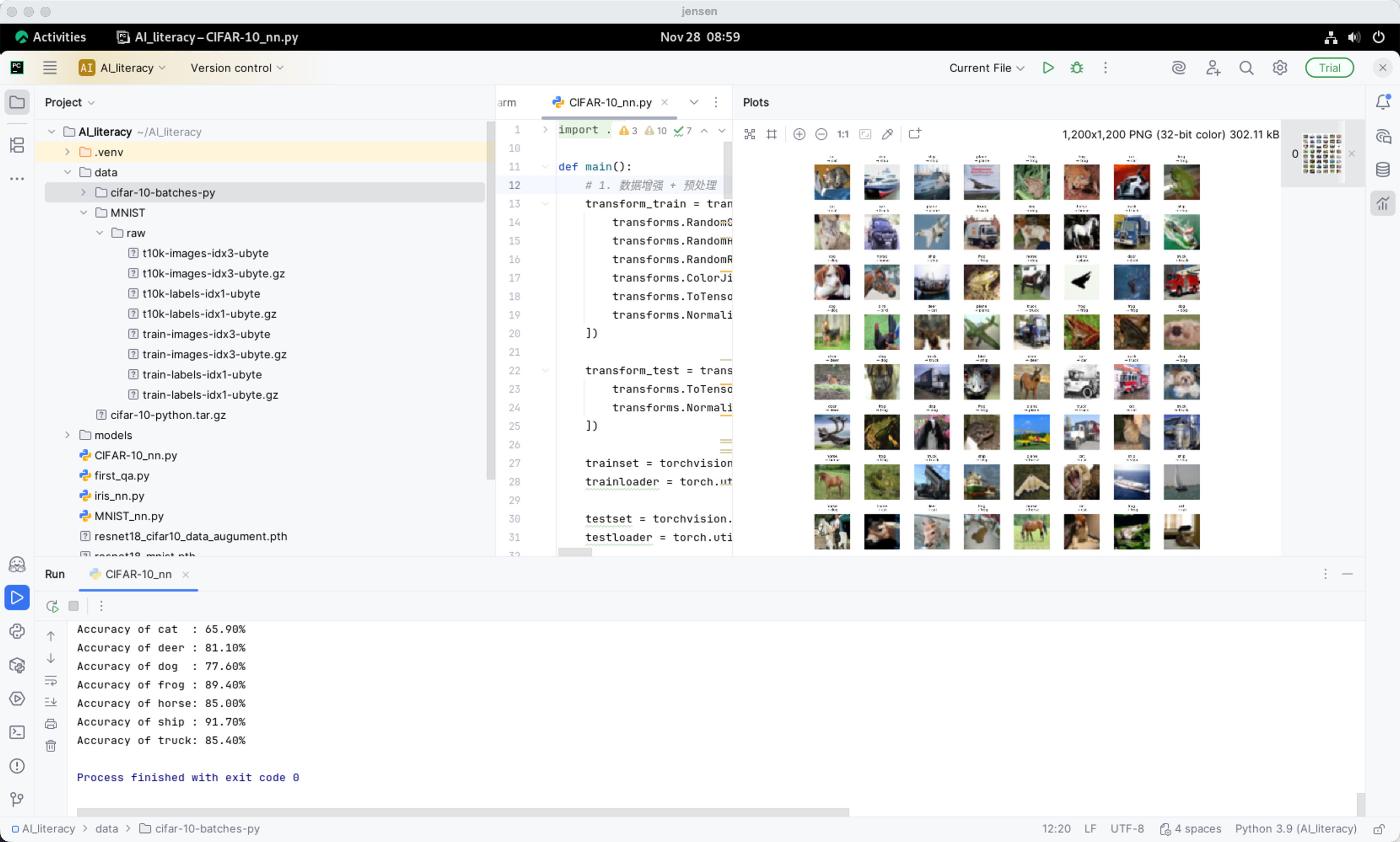
>
>
### 常见问题解答(FAQ)
**Q1: 为什么不用 `transforms.Resize(224)`?**
- **关键点**:是否使用预训练权重。
- 若 `weights=None`(从头训练)→ **不需要 Resize**,可直接用 32×32 输入。
- 若 `weights=ResNet18_Weights.DEFAULT` → 必须 Resize 到 ≥224×224,或修改首层卷积核。
> 本项目选择从头训练,故保留原始分辨率,避免信息失真。
------
**Q2: 如何解读 `_, predicted = torch.max(outputs, 1)`?**
- `outputs`:形状为 `(N, 10)` 的 logits 张量。
- `torch.max(..., dim=1)`:沿类别维度(dim=1)找最大值。
- 返回 `(values, indices)`
- `_` 忽略最大值,`predicted` 保留类别索引(0~9)
> 示例:若输出 `[2.1, 4.2, ..., 3.3]`,则 `predicted = 1`(对应 "automobile")
------
**Q3: 每类准确率是如何计算的?**
通过遍历测试集,对每个样本:
1. 判断 `predicted == label`
2. 累加到对应类别的 `class_correct[label]`
3. 同时累加 `class_total[label]`
最终:`accuracy[i] = class_correct[i] / class_total[i]`
> 这能揭示模型弱点(如“猫”类准确率显著偏低)。
### 与 Baseline 对比总结
| 方法 | 准确率 | 是否超越 82%? |
| ----------------------------- | ---------- | -------------- |
| 原始简易 CNN | 76.77% | ❌ |
| **本项目(ResNet18 + 增强)** | **83.57%** | ✅ |
| cuda-convnet(无增强) | 82% | — |
| cuda-convnet(有增强) | 89% | ⚠️ 仍有差距 |
> 下一步可尝试:MixUp、Cutout、Label Smoothing、更大模型(如 ResNet50)、迁移学习等。
------
> 附录:ImageNet Top-5 错误率演进(参考)
>
> 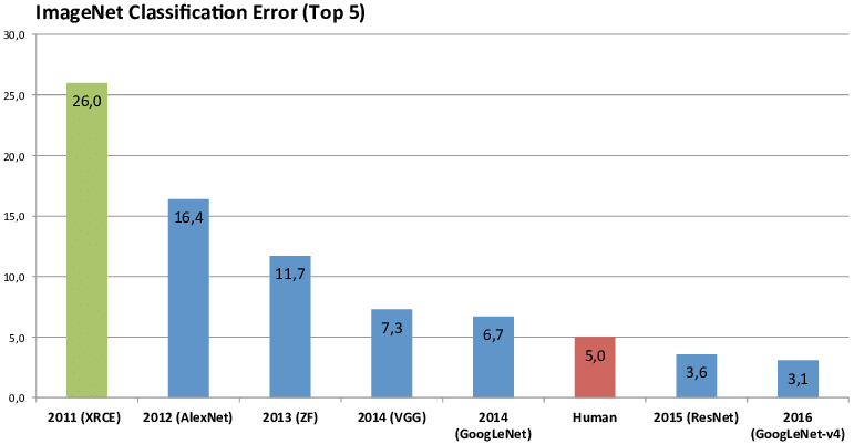
>
> - **2012 AlexNet**:开启深度学习时代(16.4% < 26%)
> - **2015 ResNet**:首次超越人类(3.6% < 5.0%)
> - **Top-5 定义**:只要真实标签在模型预测的前5名中,即视为正确。
### 结论
通过合理使用 **现代网络架构(ResNet18)** + **充分的数据增强** + **学习率调度**,我们在 CIFAR-10 上轻松超越了早期 CNN 基线,验证了“更强模型 + 更好训练策略 = 更高性能”的原则。
## 4.5 基于 ResNet50 的 Tiny ImageNet 图像分类
本项目演示如何使用 **PyTorch** 和 **torchvision** 在 **Tiny ImageNet** 数据集上微调 **预训练 ResNet50 模型**,完成图像分类任务。尽管 Tiny ImageNet(约 500MB)远小于完整 ImageNet(150GB+),但仍需合理配置数据路径、批大小(batch size)和设备资源。我们在 Apple Silicon(MPS 后端)上成功完成 25 轮训练,验证准确率达 **80.14%**,耗时约 4.5 小时。
### 1. 背景知识
#### 1.1 为什么选择 Tiny ImageNet?
| 特性 | ImageNet | Tiny ImageNet |
| -------- | ------------------------ | ----------------- |
| 类别数 | 1,000 | 200 |
| 训练图像 | ~128 万张 | 10 万张(500/类) |
| 验证图像 | 5 万张 | 1 万张(50/类) |
| 图像尺寸 | 通常 224×224(原始更大) | 固定 64×64 |
| 磁盘占用 | ~150 GB | ~250 MB(压缩后) |
Tiny ImageNet 保留了 ImageNet 的语义多样性,同时大幅降低计算开销,非常适合教学、原型验证和本地调试。
#### 1.2 为什么使用 ResNet50?
ResNet50 是由 He et al. (2015) 提出的经典深度卷积网络,其核心创新是**残差连接(skip connection)**,有效缓解了深层网络中的梯度消失与退化问题。
- **结构**:50 层(含卷积、池化、全连接)
- **输入尺寸**:224×224(需对 64×64 图像进行上采样)
- **迁移学习优势**:在 ImageNet 上预训练的权重可显著加速收敛
- **输出层**:默认 1000 类 → 微调为 200 类
------
### 2. 数据准备
#### 2.1 下载与预处理
官方数据集地址:
```bash
wget http://cs231n.stanford.edu/tiny-imagenet-200.zip
```
> 或者直接下载预处理好的数据。
>
> tiny-imagenet-200.zip, https://disk.pku.edu.cn/link/AA068C93E37D564808A74B8F282DCE0F11
> Name: tiny-imagenet-200.zip
> Expires: Never
解压后,`val/` 目录下的所有图像位于同一文件夹,不符合 `torchvision.datasets.ImageFolder` 的要求(需按类别分目录)。我们提供自动化脚本 `tinyimagenet.sh` 完成整理:
```bash
#!/bin/bash
# download and unzip dataset
#wget http://cs231n.stanford.edu/tiny-imagenet-200.zip
unzip tiny-imagenet-200.zip
current="$(pwd)/tiny-imagenet-200"
# training data
cd $current/train
for DIR in $(ls); do
cd $DIR
rm *.txt
mv images/* .
rm -r images
cd ..
done
# validation data
cd $current/val
annotate_file="val_annotations.txt"
length=$(cat $annotate_file | wc -l)
for i in $(seq 1 $length); do
# fetch i th line
line=$(sed -n ${i}p $annotate_file)
# get file name and directory name
file=$(echo $line | cut -f1 -d" " )
directory=$(echo $line | cut -f2 -d" ")
mkdir -p $directory
mv images/$file $directory
done
rm -r images
echo "done"
```
运行后目录结构如下:
```
tiny-imagenet-200/
├── train/ # 200 个子目录,每类 500 张图
├── val/ # 200 个子目录,每类 50 张图
├── test/ # 无标签(用于竞赛)
├── wnids.txt # 类别 ID 列表
└── words.txt # 类别名称映射
```
> 总大小约 **472 MB**。
------
### 3. 模型训练
#### 3.1 环境与硬件
- **设备**:Mac Studio (Apple M1 Ultra, 64GB 统一内存)
- **PyTorch 后端**:MPS(Metal Performance Shaders)
- **关键限制**:MPS **不支持 float64**,需显式使用 `.float()`
#### 3.2 完整代码
`tiny_imagenet_resnet50_epoch25.py`
```python
import os
import copy
import torch
import torch.nn as nn
import torch.optim as optim
from torchvision import datasets, models, transforms
# 训练和验证函数
def train_model(model, criterion, optimizer, scheduler, dataloaders, dataset_sizes, num_epochs=25, device='cpu'):
best_model_wts = copy.deepcopy(model.state_dict())
best_acc = 0.0
for epoch in range(num_epochs):
print('Epoch {}/{}'.format(epoch+1, num_epochs))
print('-' * 10)
# 每个 epoch 分为训练和验证阶段
for phase in ['train', 'val']:
if phase == 'train':
model.train() # 设置为训练模式
else:
model.eval() # 设置为评估模式
running_loss = 0.0
running_corrects = 0
# 遍历数据
for inputs, labels in dataloaders[phase]:
inputs = inputs.to(device)
labels = labels.to(device)
optimizer.zero_grad() # 梯度清零
# 前向传播
with torch.set_grad_enabled(phase == 'train'):
outputs = model(inputs)
_, preds = torch.max(outputs, 1)
loss = criterion(outputs, labels)
# 仅在训练阶段反向传播与参数更新
if phase == 'train':
loss.backward()
optimizer.step()
running_loss += loss.item() * inputs.size(0)
running_corrects += torch.sum(preds == labels.data)
if phase == 'train':
scheduler.step()
epoch_loss = running_loss / dataset_sizes[phase]
# MPS 后端不支持 float64 运算。解决方法是使用 float32,即调用 .float()。
#epoch_acc = running_corrects.double() / dataset_sizes[phase]
epoch_acc = running_corrects.float() / dataset_sizes[phase]
print('{} Loss: {:.4f} Acc: {:.4f}'.format(phase, epoch_loss, epoch_acc))
# 保存最佳模型参数
if phase == 'val' and epoch_acc > best_acc:
best_acc = epoch_acc
best_model_wts = copy.deepcopy(model.state_dict())
print()
print('Best val Acc: {:.4f}'.format(best_acc))
model.load_state_dict(best_model_wts)
return model
def main():
# 1. 数据预处理与加载
# 注意:此处假定ImageNet数据集按照train/val文件夹分别存放各类别图片,
# 且每个类别作为一个子文件夹存在
data_transforms = {
'train': transforms.Compose([
transforms.RandomResizedCrop(224), # 随机裁剪为224×224
transforms.RandomHorizontalFlip(), # 随机水平翻转
transforms.ToTensor(), # 转为Tensor
transforms.Normalize([0.485, 0.456, 0.406], # ImageNet均值
[0.229, 0.224, 0.225]) # ImageNet标准差
]),
'val': transforms.Compose([
transforms.Resize(256),
transforms.CenterCrop(224), # 中心裁剪
transforms.ToTensor(),
transforms.Normalize([0.485, 0.456, 0.406],
[0.229, 0.224, 0.225])
]),
}
# Tiny ImageNet 数据路径
data_dir = '/Users/hfyan/data/tiny-imagenet-200'
image_datasets = {x: datasets.ImageFolder(os.path.join(data_dir, x),
data_transforms[x])
for x in ['train', 'val']}
# 设置 num_workers 为 8 以利用多进程数据加载
dataloaders = {x: torch.utils.data.DataLoader(image_datasets[x],
batch_size=128, # 可根据实际情况调整
shuffle=True,
num_workers=8)
for x in ['train', 'val']}
dataset_sizes = {x: len(image_datasets[x]) for x in ['train', 'val']}
class_names = image_datasets['train'].classes
#device = torch.device("cuda:0" if torch.cuda.is_available() else "cpu")
# 使用 MPS 作为 GPU 后端(适用于 Apple Silicon)
if torch.backends.mps.is_available():
device = torch.device("mps")
print("Using MPS device for GPU acceleration")
else:
device = torch.device("cpu")
print("MPS device not available, using CPU")
#2. 构建模型(使用预训练 ResNet50)
# 这里我们加载预训练的 ResNet50 模型,并修改最后的全连接层以适应Tiny ImageNet的类别数(200类)
model_ft = models.resnet50(weights=models.ResNet50_Weights.DEFAULT)
num_ftrs = model_ft.fc.in_features
model_ft.fc = nn.Linear(num_ftrs, len(class_names))
model_ft = model_ft.to(device)
criterion = nn.CrossEntropyLoss()
optimizer_ft = optim.SGD(model_ft.parameters(), lr=0.001, momentum=0.9)
# 学习率调整策略,每7个epoch降低一次学习率
exp_lr_scheduler = optim.lr_scheduler.StepLR(optimizer_ft, step_size=7, gamma=0.1)
#3. 训练模型
num_epochs = 25 # 可根据需要调整epoch数量
model_ft = train_model(model_ft, criterion, optimizer_ft, exp_lr_scheduler,
dataloaders, dataset_sizes, num_epochs=num_epochs, device=device)
#4. 保存模型,文件名建议为 tiny_imagenet_resnet50_epoch25.pth
torch.save(model_ft.state_dict(), 'tiny_imagenet_resnet50_epoch25.pth')
print("Model saved as tiny_imagenet_resnet50_epoch25.pth")
if __name__ == '__main__':
main()
```
> **说明**
>
> - **数据预处理**
> 使用了 `transforms` 对数据进行了数据增强(如随机裁剪、水平翻转)以及归一化(ImageNet常用的均值和标准差)。数据文件夹需要符合 `ImageFolder` 的要求,每个类别存放在独立的子文件夹中。
> - **模型构建**
> 本示例中采用预训练的 ResNet50 模型,并修改了最后一层全连接层以输出与类别数匹配的概率分布。
> - **训练过程**
> 代码中定义了 `train_model` 函数,对模型进行训练和验证,并在验证集上选取准确率最高的模型参数。学习率调度器用于逐步降低学习率以便更好地收敛。
> - **注意事项**
> - ImageNet 数据集较大,建议在使用时注意数据加载、内存管理和训练时长。
> - 如需更深入的模型调优或使用分布式训练,请参考 PyTorch 官方文档和相关资料。
>
> 该示例代码为入门级示例,实际项目中可能需要更多的优化和配置。
>
>
>
> **主入口保护**:所有涉及多进程或多线程的代码都封装在 `if __name__ == '__main__':` 下,避免 macOS 下的启动问题。
**2025/2/24 11:30开始运行,16:00结束**
> File "/Users/hfyan/data/tiny_imagenet_resnet50_epoch25.py", line 47, in train_model
>
> epoch_acc = running_corrects.double() / dataset_sizes[phase]
>
> TypeError: Cannot convert a MPS Tensor to float64 dtype as the MPS framework doesn't support float64. Please use float32 instead.
>
> (base) hfyan@HongfeideMac-Studio data % python tiny_imagenet_resnet50_epoch25.py
```
(base) hfyan@HongfeideMac-Studio data % python tiny_imagenet_resnet50_epoch25.py
Using MPS device for GPU acceleration
Epoch 1/25
----------
train Loss: 5.0366 Acc: 0.0720
val Loss: 4.1348 Acc: 0.2819
Epoch 2/25
----------
train Loss: 3.2563 Acc: 0.3406
val Loss: 1.7006 Acc: 0.6197
Epoch 3/25
----------
train Loss: 2.1834 Acc: 0.5065
val Loss: 1.2068 Acc: 0.7062
Epoch 4/25
----------
train Loss: 1.8635 Acc: 0.5663
val Loss: 1.0010 Acc: 0.7498
Epoch 5/25
----------
train Loss: 1.6788 Acc: 0.6029
val Loss: 0.8927 Acc: 0.7702
Epoch 6/25
----------
train Loss: 1.5723 Acc: 0.6268
val Loss: 0.8407 Acc: 0.7808
Epoch 7/25
----------
train Loss: 1.5044 Acc: 0.6390
val Loss: 0.7990 Acc: 0.7907
Epoch 8/25
----------
train Loss: 1.4324 Acc: 0.6567
val Loss: 0.7788 Acc: 0.7939
Epoch 9/25
----------
train Loss: 1.4212 Acc: 0.6571
val Loss: 0.7701 Acc: 0.7981
Epoch 10/25
----------
train Loss: 1.4054 Acc: 0.6614
val Loss: 0.7669 Acc: 0.7966
Epoch 11/25
----------
train Loss: 1.4035 Acc: 0.6615
val Loss: 0.7634 Acc: 0.7980
Epoch 12/25
----------
train Loss: 1.3995 Acc: 0.6626
val Loss: 0.7595 Acc: 0.7990
Epoch 13/25
----------
train Loss: 1.3882 Acc: 0.6647
val Loss: 0.7558 Acc: 0.7988
Epoch 14/25
----------
train Loss: 1.3747 Acc: 0.6680
val Loss: 0.7517 Acc: 0.7997
Epoch 15/25
----------
train Loss: 1.3754 Acc: 0.6683
val Loss: 0.7490 Acc: 0.8006
Epoch 16/25
----------
train Loss: 1.3685 Acc: 0.6689
val Loss: 0.7592 Acc: 0.7970
Epoch 17/25
----------
train Loss: 1.3771 Acc: 0.6681
val Loss: 0.7567 Acc: 0.8009
Epoch 18/25
----------
train Loss: 1.3690 Acc: 0.6688
val Loss: 0.7508 Acc: 0.8011
Epoch 19/25
----------
train Loss: 1.3716 Acc: 0.6694
val Loss: 0.7521 Acc: 0.8008
Epoch 20/25
----------
train Loss: 1.3729 Acc: 0.6687
val Loss: 0.7527 Acc: 0.8002
Epoch 21/25
----------
train Loss: 1.3709 Acc: 0.6689
val Loss: 0.7501 Acc: 0.8014
Epoch 22/25
----------
train Loss: 1.3706 Acc: 0.6708
val Loss: 0.7516 Acc: 0.8008
Epoch 23/25
----------
train Loss: 1.3681 Acc: 0.6696
val Loss: 0.7502 Acc: 0.8002
Epoch 24/25
----------
train Loss: 1.3725 Acc: 0.6698
val Loss: 0.7508 Acc: 0.8003
Epoch 25/25
----------
train Loss: 1.3708 Acc: 0.6696
val Loss: 0.7480 Acc: 0.8004
Best val Acc: 0.8014
Model saved as tiny_imagenet_resnet50_epoch25.pth
```
跑了4小时30分钟。
> 结果如下:
>
> ```
> /home/rocky/AI_literacy/.venv/bin/python /home/rocky/AI_literacy/CIFAR-10_nn.py
> 100%|██████████| 170M/170M [00:15<00:00, 11.1MB/s]
> /usr/lib64/python3.9/tarfile.py:2288: RuntimeWarning: The default behavior of tarfile extraction has been changed to disallow common exploits (including CVE-2007-4559). By default, absolute/parent paths are disallowed and some mode bits are cleared. See https://access.redhat.com/articles/7004769 for more details.
> warnings.warn(
> Using device: cpu
> Starting training with early stopping...
> /home/rocky/AI_literacy/.venv/lib64/python3.9/site-packages/torch/utils/data/dataloader.py:666: UserWarning: 'pin_memory' argument is set as true but no accelerator is found, then device pinned memory won't be used.
> warnings.warn(warn_msg)
> [1, 100] loss: 1.893
> [1, 200] loss: 1.658
> [1, 300] loss: 1.698
> [1] Avg Loss: 1.804
> [2, 100] loss: 1.399
> [2, 200] loss: 1.580
> [2, 300] loss: 1.407
> [2] Avg Loss: 1.517
> [3, 100] loss: 1.346
> [3, 200] loss: 1.492
> [3, 300] loss: 1.097
> [3] Avg Loss: 1.373
> [4, 100] loss: 1.309
> [4, 200] loss: 1.182
> [4, 300] loss: 1.187
> [4] Avg Loss: 1.244
> [5, 100] loss: 1.104
> [5, 200] loss: 1.084
> [5, 300] loss: 1.081
> [5] Avg Loss: 1.151
> ......
> [267, 100] loss: 0.278
> [267, 200] loss: 0.226
> [267, 300] loss: 0.188
> [267] Avg Loss: 0.249
> [268, 100] loss: 0.218
> [268, 200] loss: 0.220
> [268, 300] loss: 0.206
> [268] Avg Loss: 0.256
> No improvement. Patience: 1/10
> [269, 100] loss: 0.200
> [269, 200] loss: 0.175
> [269, 300] loss: 0.298
> [269] Avg Loss: 0.256
> No improvement. Patience: 2/10
> [270, 100] loss: 0.325
> [270, 200] loss: 0.265
> [270, 300] loss: 0.319
> [270] Avg Loss: 0.258
> No improvement. Patience: 3/10
> [271, 100] loss: 0.316
> [271, 200] loss: 0.139
> [271, 300] loss: 0.263
> [271] Avg Loss: 0.251
> No improvement. Patience: 4/10
> [272, 100] loss: 0.260
> [272, 200] loss: 0.184
> [272, 300] loss: 0.141
> [272] Avg Loss: 0.256
> No improvement. Patience: 5/10
> [273, 100] loss: 0.263
> [273, 200] loss: 0.327
> [273, 300] loss: 0.246
> [273] Avg Loss: 0.250
> No improvement. Patience: 6/10
> [274, 100] loss: 0.193
> [274, 200] loss: 0.221
> [274, 300] loss: 0.227
> [274] Avg Loss: 0.250
> No improvement. Patience: 7/10
> [275, 100] loss: 0.185
> [275, 200] loss: 0.354
> [275, 300] loss: 0.254
> [275] Avg Loss: 0.258
> No improvement. Patience: 8/10
> [276, 100] loss: 0.354
> [276, 200] loss: 0.326
> [276, 300] loss: 0.246
> [276] Avg Loss: 0.250
> No improvement. Patience: 9/10
> [277, 100] loss: 0.183
> [277, 200] loss: 0.383
> [277, 300] loss: 0.295
> [277] Avg Loss: 0.256
> No improvement. Patience: 10/10
> Early stopping triggered.
> ✅ Training completed in 636.54 minutes.
> Accuracy on test images: 83.67%
> Accuracy of plane: 84.70%
> Accuracy of car : 91.90%
> Accuracy of bird : 84.00%
> Accuracy of cat : 65.90%
> Accuracy of deer : 81.10%
> Accuracy of dog : 77.60%
> Accuracy of frog : 89.40%
> Accuracy of horse: 85.00%
> Accuracy of ship : 91.70%
> Accuracy of truck: 85.40%
>
> Process finished with exit code 0
>
> ```
>
>
>
> 
>
>
### 常见问题解答(FAQ)
**Q1: 为什么不用 `transforms.Resize(224)`?**
- **关键点**:是否使用预训练权重。
- 若 `weights=None`(从头训练)→ **不需要 Resize**,可直接用 32×32 输入。
- 若 `weights=ResNet18_Weights.DEFAULT` → 必须 Resize 到 ≥224×224,或修改首层卷积核。
> 本项目选择从头训练,故保留原始分辨率,避免信息失真。
------
**Q2: 如何解读 `_, predicted = torch.max(outputs, 1)`?**
- `outputs`:形状为 `(N, 10)` 的 logits 张量。
- `torch.max(..., dim=1)`:沿类别维度(dim=1)找最大值。
- 返回 `(values, indices)`
- `_` 忽略最大值,`predicted` 保留类别索引(0~9)
> 示例:若输出 `[2.1, 4.2, ..., 3.3]`,则 `predicted = 1`(对应 "automobile")
------
**Q3: 每类准确率是如何计算的?**
通过遍历测试集,对每个样本:
1. 判断 `predicted == label`
2. 累加到对应类别的 `class_correct[label]`
3. 同时累加 `class_total[label]`
最终:`accuracy[i] = class_correct[i] / class_total[i]`
> 这能揭示模型弱点(如“猫”类准确率显著偏低)。
### 与 Baseline 对比总结
| 方法 | 准确率 | 是否超越 82%? |
| ----------------------------- | ---------- | -------------- |
| 原始简易 CNN | 76.77% | ❌ |
| **本项目(ResNet18 + 增强)** | **83.57%** | ✅ |
| cuda-convnet(无增强) | 82% | — |
| cuda-convnet(有增强) | 89% | ⚠️ 仍有差距 |
> 下一步可尝试:MixUp、Cutout、Label Smoothing、更大模型(如 ResNet50)、迁移学习等。
------
> 附录:ImageNet Top-5 错误率演进(参考)
>
> 
>
> - **2012 AlexNet**:开启深度学习时代(16.4% < 26%)
> - **2015 ResNet**:首次超越人类(3.6% < 5.0%)
> - **Top-5 定义**:只要真实标签在模型预测的前5名中,即视为正确。
### 结论
通过合理使用 **现代网络架构(ResNet18)** + **充分的数据增强** + **学习率调度**,我们在 CIFAR-10 上轻松超越了早期 CNN 基线,验证了“更强模型 + 更好训练策略 = 更高性能”的原则。
## 4.5 基于 ResNet50 的 Tiny ImageNet 图像分类
本项目演示如何使用 **PyTorch** 和 **torchvision** 在 **Tiny ImageNet** 数据集上微调 **预训练 ResNet50 模型**,完成图像分类任务。尽管 Tiny ImageNet(约 500MB)远小于完整 ImageNet(150GB+),但仍需合理配置数据路径、批大小(batch size)和设备资源。我们在 Apple Silicon(MPS 后端)上成功完成 25 轮训练,验证准确率达 **80.14%**,耗时约 4.5 小时。
### 1. 背景知识
#### 1.1 为什么选择 Tiny ImageNet?
| 特性 | ImageNet | Tiny ImageNet |
| -------- | ------------------------ | ----------------- |
| 类别数 | 1,000 | 200 |
| 训练图像 | ~128 万张 | 10 万张(500/类) |
| 验证图像 | 5 万张 | 1 万张(50/类) |
| 图像尺寸 | 通常 224×224(原始更大) | 固定 64×64 |
| 磁盘占用 | ~150 GB | ~250 MB(压缩后) |
Tiny ImageNet 保留了 ImageNet 的语义多样性,同时大幅降低计算开销,非常适合教学、原型验证和本地调试。
#### 1.2 为什么使用 ResNet50?
ResNet50 是由 He et al. (2015) 提出的经典深度卷积网络,其核心创新是**残差连接(skip connection)**,有效缓解了深层网络中的梯度消失与退化问题。
- **结构**:50 层(含卷积、池化、全连接)
- **输入尺寸**:224×224(需对 64×64 图像进行上采样)
- **迁移学习优势**:在 ImageNet 上预训练的权重可显著加速收敛
- **输出层**:默认 1000 类 → 微调为 200 类
------
### 2. 数据准备
#### 2.1 下载与预处理
官方数据集地址:
```bash
wget http://cs231n.stanford.edu/tiny-imagenet-200.zip
```
> 或者直接下载预处理好的数据。
>
> tiny-imagenet-200.zip, https://disk.pku.edu.cn/link/AA068C93E37D564808A74B8F282DCE0F11
> Name: tiny-imagenet-200.zip
> Expires: Never
解压后,`val/` 目录下的所有图像位于同一文件夹,不符合 `torchvision.datasets.ImageFolder` 的要求(需按类别分目录)。我们提供自动化脚本 `tinyimagenet.sh` 完成整理:
```bash
#!/bin/bash
# download and unzip dataset
#wget http://cs231n.stanford.edu/tiny-imagenet-200.zip
unzip tiny-imagenet-200.zip
current="$(pwd)/tiny-imagenet-200"
# training data
cd $current/train
for DIR in $(ls); do
cd $DIR
rm *.txt
mv images/* .
rm -r images
cd ..
done
# validation data
cd $current/val
annotate_file="val_annotations.txt"
length=$(cat $annotate_file | wc -l)
for i in $(seq 1 $length); do
# fetch i th line
line=$(sed -n ${i}p $annotate_file)
# get file name and directory name
file=$(echo $line | cut -f1 -d" " )
directory=$(echo $line | cut -f2 -d" ")
mkdir -p $directory
mv images/$file $directory
done
rm -r images
echo "done"
```
运行后目录结构如下:
```
tiny-imagenet-200/
├── train/ # 200 个子目录,每类 500 张图
├── val/ # 200 个子目录,每类 50 张图
├── test/ # 无标签(用于竞赛)
├── wnids.txt # 类别 ID 列表
└── words.txt # 类别名称映射
```
> 总大小约 **472 MB**。
------
### 3. 模型训练
#### 3.1 环境与硬件
- **设备**:Mac Studio (Apple M1 Ultra, 64GB 统一内存)
- **PyTorch 后端**:MPS(Metal Performance Shaders)
- **关键限制**:MPS **不支持 float64**,需显式使用 `.float()`
#### 3.2 完整代码
`tiny_imagenet_resnet50_epoch25.py`
```python
import os
import copy
import torch
import torch.nn as nn
import torch.optim as optim
from torchvision import datasets, models, transforms
# 训练和验证函数
def train_model(model, criterion, optimizer, scheduler, dataloaders, dataset_sizes, num_epochs=25, device='cpu'):
best_model_wts = copy.deepcopy(model.state_dict())
best_acc = 0.0
for epoch in range(num_epochs):
print('Epoch {}/{}'.format(epoch+1, num_epochs))
print('-' * 10)
# 每个 epoch 分为训练和验证阶段
for phase in ['train', 'val']:
if phase == 'train':
model.train() # 设置为训练模式
else:
model.eval() # 设置为评估模式
running_loss = 0.0
running_corrects = 0
# 遍历数据
for inputs, labels in dataloaders[phase]:
inputs = inputs.to(device)
labels = labels.to(device)
optimizer.zero_grad() # 梯度清零
# 前向传播
with torch.set_grad_enabled(phase == 'train'):
outputs = model(inputs)
_, preds = torch.max(outputs, 1)
loss = criterion(outputs, labels)
# 仅在训练阶段反向传播与参数更新
if phase == 'train':
loss.backward()
optimizer.step()
running_loss += loss.item() * inputs.size(0)
running_corrects += torch.sum(preds == labels.data)
if phase == 'train':
scheduler.step()
epoch_loss = running_loss / dataset_sizes[phase]
# MPS 后端不支持 float64 运算。解决方法是使用 float32,即调用 .float()。
#epoch_acc = running_corrects.double() / dataset_sizes[phase]
epoch_acc = running_corrects.float() / dataset_sizes[phase]
print('{} Loss: {:.4f} Acc: {:.4f}'.format(phase, epoch_loss, epoch_acc))
# 保存最佳模型参数
if phase == 'val' and epoch_acc > best_acc:
best_acc = epoch_acc
best_model_wts = copy.deepcopy(model.state_dict())
print()
print('Best val Acc: {:.4f}'.format(best_acc))
model.load_state_dict(best_model_wts)
return model
def main():
# 1. 数据预处理与加载
# 注意:此处假定ImageNet数据集按照train/val文件夹分别存放各类别图片,
# 且每个类别作为一个子文件夹存在
data_transforms = {
'train': transforms.Compose([
transforms.RandomResizedCrop(224), # 随机裁剪为224×224
transforms.RandomHorizontalFlip(), # 随机水平翻转
transforms.ToTensor(), # 转为Tensor
transforms.Normalize([0.485, 0.456, 0.406], # ImageNet均值
[0.229, 0.224, 0.225]) # ImageNet标准差
]),
'val': transforms.Compose([
transforms.Resize(256),
transforms.CenterCrop(224), # 中心裁剪
transforms.ToTensor(),
transforms.Normalize([0.485, 0.456, 0.406],
[0.229, 0.224, 0.225])
]),
}
# Tiny ImageNet 数据路径
data_dir = '/Users/hfyan/data/tiny-imagenet-200'
image_datasets = {x: datasets.ImageFolder(os.path.join(data_dir, x),
data_transforms[x])
for x in ['train', 'val']}
# 设置 num_workers 为 8 以利用多进程数据加载
dataloaders = {x: torch.utils.data.DataLoader(image_datasets[x],
batch_size=128, # 可根据实际情况调整
shuffle=True,
num_workers=8)
for x in ['train', 'val']}
dataset_sizes = {x: len(image_datasets[x]) for x in ['train', 'val']}
class_names = image_datasets['train'].classes
#device = torch.device("cuda:0" if torch.cuda.is_available() else "cpu")
# 使用 MPS 作为 GPU 后端(适用于 Apple Silicon)
if torch.backends.mps.is_available():
device = torch.device("mps")
print("Using MPS device for GPU acceleration")
else:
device = torch.device("cpu")
print("MPS device not available, using CPU")
#2. 构建模型(使用预训练 ResNet50)
# 这里我们加载预训练的 ResNet50 模型,并修改最后的全连接层以适应Tiny ImageNet的类别数(200类)
model_ft = models.resnet50(weights=models.ResNet50_Weights.DEFAULT)
num_ftrs = model_ft.fc.in_features
model_ft.fc = nn.Linear(num_ftrs, len(class_names))
model_ft = model_ft.to(device)
criterion = nn.CrossEntropyLoss()
optimizer_ft = optim.SGD(model_ft.parameters(), lr=0.001, momentum=0.9)
# 学习率调整策略,每7个epoch降低一次学习率
exp_lr_scheduler = optim.lr_scheduler.StepLR(optimizer_ft, step_size=7, gamma=0.1)
#3. 训练模型
num_epochs = 25 # 可根据需要调整epoch数量
model_ft = train_model(model_ft, criterion, optimizer_ft, exp_lr_scheduler,
dataloaders, dataset_sizes, num_epochs=num_epochs, device=device)
#4. 保存模型,文件名建议为 tiny_imagenet_resnet50_epoch25.pth
torch.save(model_ft.state_dict(), 'tiny_imagenet_resnet50_epoch25.pth')
print("Model saved as tiny_imagenet_resnet50_epoch25.pth")
if __name__ == '__main__':
main()
```
> **说明**
>
> - **数据预处理**
> 使用了 `transforms` 对数据进行了数据增强(如随机裁剪、水平翻转)以及归一化(ImageNet常用的均值和标准差)。数据文件夹需要符合 `ImageFolder` 的要求,每个类别存放在独立的子文件夹中。
> - **模型构建**
> 本示例中采用预训练的 ResNet50 模型,并修改了最后一层全连接层以输出与类别数匹配的概率分布。
> - **训练过程**
> 代码中定义了 `train_model` 函数,对模型进行训练和验证,并在验证集上选取准确率最高的模型参数。学习率调度器用于逐步降低学习率以便更好地收敛。
> - **注意事项**
> - ImageNet 数据集较大,建议在使用时注意数据加载、内存管理和训练时长。
> - 如需更深入的模型调优或使用分布式训练,请参考 PyTorch 官方文档和相关资料。
>
> 该示例代码为入门级示例,实际项目中可能需要更多的优化和配置。
>
>
>
> **主入口保护**:所有涉及多进程或多线程的代码都封装在 `if __name__ == '__main__':` 下,避免 macOS 下的启动问题。
**2025/2/24 11:30开始运行,16:00结束**
> File "/Users/hfyan/data/tiny_imagenet_resnet50_epoch25.py", line 47, in train_model
>
> epoch_acc = running_corrects.double() / dataset_sizes[phase]
>
> TypeError: Cannot convert a MPS Tensor to float64 dtype as the MPS framework doesn't support float64. Please use float32 instead.
>
> (base) hfyan@HongfeideMac-Studio data % python tiny_imagenet_resnet50_epoch25.py
```
(base) hfyan@HongfeideMac-Studio data % python tiny_imagenet_resnet50_epoch25.py
Using MPS device for GPU acceleration
Epoch 1/25
----------
train Loss: 5.0366 Acc: 0.0720
val Loss: 4.1348 Acc: 0.2819
Epoch 2/25
----------
train Loss: 3.2563 Acc: 0.3406
val Loss: 1.7006 Acc: 0.6197
Epoch 3/25
----------
train Loss: 2.1834 Acc: 0.5065
val Loss: 1.2068 Acc: 0.7062
Epoch 4/25
----------
train Loss: 1.8635 Acc: 0.5663
val Loss: 1.0010 Acc: 0.7498
Epoch 5/25
----------
train Loss: 1.6788 Acc: 0.6029
val Loss: 0.8927 Acc: 0.7702
Epoch 6/25
----------
train Loss: 1.5723 Acc: 0.6268
val Loss: 0.8407 Acc: 0.7808
Epoch 7/25
----------
train Loss: 1.5044 Acc: 0.6390
val Loss: 0.7990 Acc: 0.7907
Epoch 8/25
----------
train Loss: 1.4324 Acc: 0.6567
val Loss: 0.7788 Acc: 0.7939
Epoch 9/25
----------
train Loss: 1.4212 Acc: 0.6571
val Loss: 0.7701 Acc: 0.7981
Epoch 10/25
----------
train Loss: 1.4054 Acc: 0.6614
val Loss: 0.7669 Acc: 0.7966
Epoch 11/25
----------
train Loss: 1.4035 Acc: 0.6615
val Loss: 0.7634 Acc: 0.7980
Epoch 12/25
----------
train Loss: 1.3995 Acc: 0.6626
val Loss: 0.7595 Acc: 0.7990
Epoch 13/25
----------
train Loss: 1.3882 Acc: 0.6647
val Loss: 0.7558 Acc: 0.7988
Epoch 14/25
----------
train Loss: 1.3747 Acc: 0.6680
val Loss: 0.7517 Acc: 0.7997
Epoch 15/25
----------
train Loss: 1.3754 Acc: 0.6683
val Loss: 0.7490 Acc: 0.8006
Epoch 16/25
----------
train Loss: 1.3685 Acc: 0.6689
val Loss: 0.7592 Acc: 0.7970
Epoch 17/25
----------
train Loss: 1.3771 Acc: 0.6681
val Loss: 0.7567 Acc: 0.8009
Epoch 18/25
----------
train Loss: 1.3690 Acc: 0.6688
val Loss: 0.7508 Acc: 0.8011
Epoch 19/25
----------
train Loss: 1.3716 Acc: 0.6694
val Loss: 0.7521 Acc: 0.8008
Epoch 20/25
----------
train Loss: 1.3729 Acc: 0.6687
val Loss: 0.7527 Acc: 0.8002
Epoch 21/25
----------
train Loss: 1.3709 Acc: 0.6689
val Loss: 0.7501 Acc: 0.8014
Epoch 22/25
----------
train Loss: 1.3706 Acc: 0.6708
val Loss: 0.7516 Acc: 0.8008
Epoch 23/25
----------
train Loss: 1.3681 Acc: 0.6696
val Loss: 0.7502 Acc: 0.8002
Epoch 24/25
----------
train Loss: 1.3725 Acc: 0.6698
val Loss: 0.7508 Acc: 0.8003
Epoch 25/25
----------
train Loss: 1.3708 Acc: 0.6696
val Loss: 0.7480 Acc: 0.8004
Best val Acc: 0.8014
Model saved as tiny_imagenet_resnet50_epoch25.pth
```
跑了4小时30分钟。
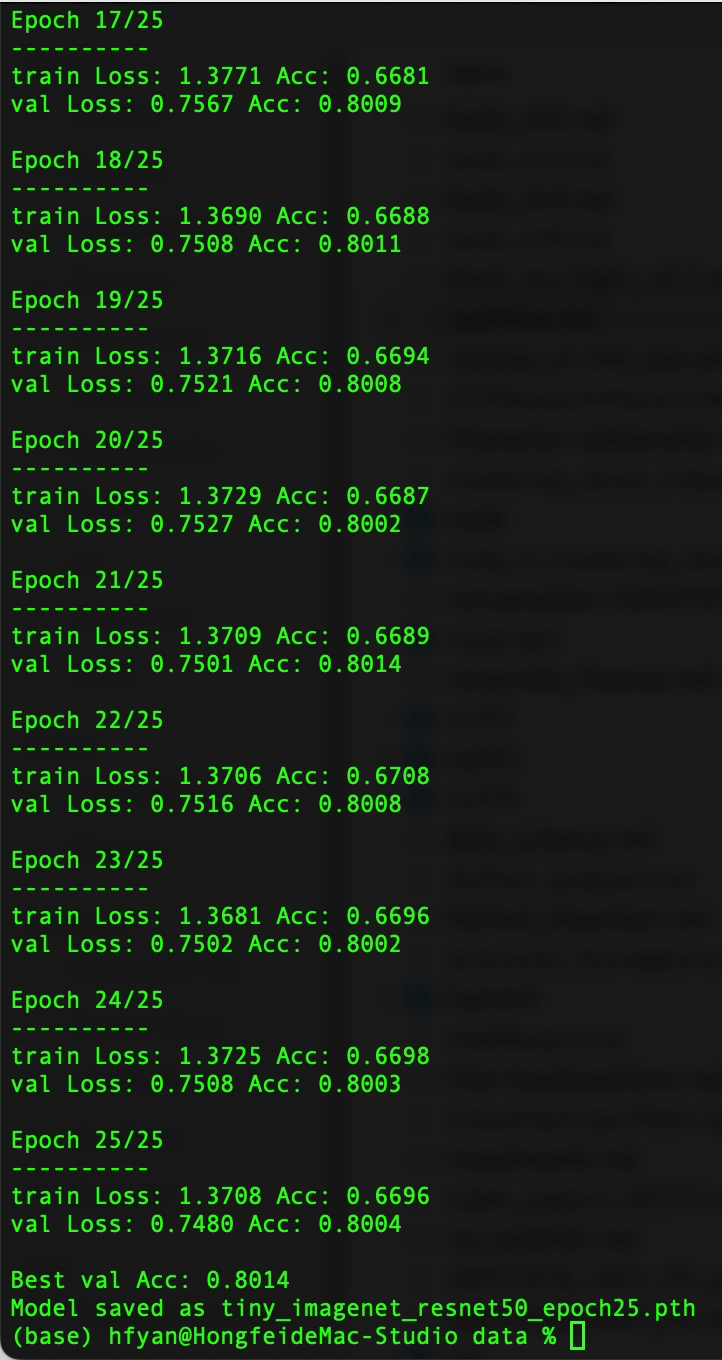 ```
% ls -lh *.pth
-rw-r--r-- 1 hfyan staff 92M Feb 24 16:02 tiny_imagenet_resnet50_epoch25.pth
```
#### 3.3 常见问题解答
##### Q1:为何每次运行都重新下载 ResNet50 权重?
PyTorch 默认缓存至 `~/.cache/torch/hub/checkpoints/`。若重复下载,请检查:
- 文件是否存在且完整(`resnet50-11ad3fa6.pth` ≈ 97MB)
- 目录写权限
- 是否使用临时环境(如容器)
可通过设置环境变量指定缓存路径:
```bash
export TORCH_HOME=/path/to/stable/cache
```
##### Q2:MPS 报错 “Cannot convert to float64”?
Apple MPS 不支持 double 精度。务必使用:
```python
accuracy = correct.float() / total # ✅ 正确
# accuracy = correct.double() / total # ❌ 错误
```
##### Q3:如何命名模型文件?
推荐格式:`{dataset}_{model}_{epochs}.pth`
示例:`tiny_imagenet_resnet50_epoch25.pth`
------
### 4. 模型评估
前面已经保存了模型权重,可以通过如下步骤加载模型并在验证集上进行评估:
1. **加载模型结构和权重**
请确保你定义的模型结构与训练时保持一致。使用 `torch.load` 加载权重,并用 `model.load_state_dict` 导入。
2. **切换到评估模式**
调用 `model.eval()` 确保模型关闭 BatchNorm、Dropout 等训练时特有的行为。
3. **遍历验证数据并计算准确率**
使用 `torch.no_grad()` 关闭梯度计算,加快验证速度,并防止内存浪费。
下面是一个完整的示例代码,`eval_tiny_imagenet_resnet50_epoch25_pth.py `:
```python
import os
import torch
import torch.nn as nn
from torchvision import datasets, models, transforms
# 数据预处理
data_transforms = {
'val': transforms.Compose([
transforms.Resize(256),
transforms.CenterCrop(224),
transforms.ToTensor(),
transforms.Normalize([0.485, 0.456, 0.406],
[0.229, 0.224, 0.225])
]),
}
# 确保子进程安全启动
if __name__ == '__main__':
data_dir = '/Users/hfyan/data/tiny-imagenet-200'
val_dir = os.path.join(data_dir, 'val')
val_dataset = datasets.ImageFolder(val_dir, data_transforms['val'])
val_loader = torch.utils.data.DataLoader(val_dataset, batch_size=64,
shuffle=False, num_workers=4)
# 选择设备
if torch.backends.mps.is_available():
device = torch.device("mps")
print("Using MPS device for GPU acceleration")
else:
device = torch.device("cpu")
print("MPS device not available, using CPU")
# 加载模型
model_ft = models.resnet50(pretrained=False)
num_ftrs = model_ft.fc.in_features
model_ft.fc = nn.Linear(num_ftrs, len(val_dataset.classes))
model_ft = model_ft.to(device)
# 加载模型权重
model_path = 'tiny_imagenet_resnet50_epoch25.pth'
model_ft.load_state_dict(torch.load(model_path, map_location=device))
# 评估模式
model_ft.eval()
# 模型评估
running_corrects = 0
total_samples = 0
with torch.no_grad():
for inputs, labels in val_loader:
inputs = inputs.to(device)
labels = labels.to(device)
outputs = model_ft(inputs)
_, preds = torch.max(outputs, 1)
running_corrects += torch.sum(preds == labels.data)
total_samples += inputs.size(0)
val_acc = running_corrects.float() / total_samples
print('Validation Accuracy: {:.4f}'.format(val_acc))
```
验证步骤:
> - 加载与你训练时一致的模型结构。
> - 使用 `model.load_state_dict()` 加载权重。
> - 调用 `model.eval()` 进入验证模式。
> - 遍历验证数据集,计算准确率或其他指标。
>
> 这样,你就可以加载已保存的模型并对验证集数据进行测试。
>
> 
>
>
>
> ```python
> (base) hfyan@HongfeideMac-Studio data % python eval_tiny_imagenet_resnet50_epoch25_pth.py
> Using MPS device for GPU acceleration
> /Users/hfyan/miniconda3/lib/python3.10/site-packages/torchvision/models/_utils.py:208: UserWarning: The parameter 'pretrained' is deprecated since 0.13 and may be removed in the future, please use 'weights' instead.
> warnings.warn(
> /Users/hfyan/miniconda3/lib/python3.10/site-packages/torchvision/models/_utils.py:223: UserWarning: Arguments other than a weight enum or `None` for 'weights' are deprecated since 0.13 and may be removed in the future. The current behavior is equivalent to passing `weights=None`.
> warnings.warn(msg)
> Validation Accuracy: 0.8014
> (base) hfyan@HongfeideMac-Studio data %
> ```
### 5. 扩展与优化
#### 5.1 性能对比:ImageNet vs Tiny ImageNet
| 指标 | ImageNet (ResNet50) | Tiny ImageNet (本实验) |
| --------- | ----------------------------- | ------------------------ |
| Top-1 Acc | ~76.5%(原始)→ 84%(优化后) | **80.14%** |
| 训练时间 | 数天(8×V100) | **4.5 小时**(M1 Ultra) |
| 显存需求 | >16 GB | <8 GB(batch=128) |
------
#### 5.2 关于多进程与 GIL
- `DataLoader(num_workers>0)` 使用 **多进程**(非线程),绕过 Python GIL
- PyTorch 底层计算(C++/CUDA/Metal)不受 GIL 限制
- 小规模任务(如小矩阵乘法)并行可能因通信开销而变慢
#### 总结
本项目完整展示了从数据准备、模型微调到评估的全流程,适合入门者理解迁移学习与 PyTorch 实践。通过合理利用 Apple Silicon 的 MPS 加速,可在消费级设备上高效完成中等规模视觉任务。
# 5.强化学习
## 5.1 Pong 游戏智能体
包含多种强化学习算法(Q-learning, DQN, A2C)用于训练 Pong 游戏智能体的仓库。本项目提供了完整的训练环境、算法实现以及可视化工具。
> 【25级工学院同学】贡献几个RL的实例,《动手学强化学习》https://hrl.boyuai.com 上的前面的算法,都用自己创建的一个乒乓球小游戏的环境在cpu上面跑通过。然后还看了一些yutube上面斯坦福的cs231n。
https://github.com/DawnTilDusk/RL-pong
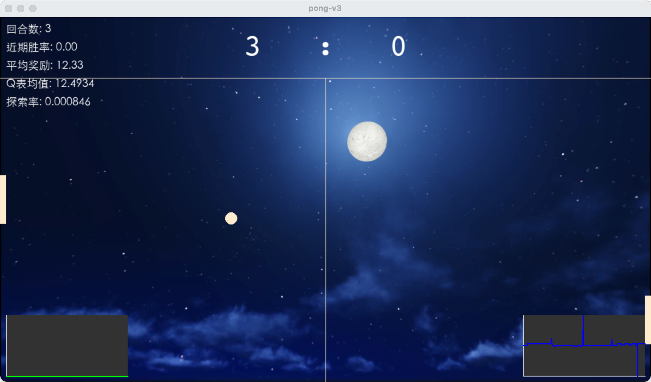
## 5.2 2048 游戏智能体
图形界面,上下左右键玩2048
https://github.com/GMyhf/2025spring-cs201/blob/main/code/2048/1_game_2048_gui.py
```
% ls -lh *.pth
-rw-r--r-- 1 hfyan staff 92M Feb 24 16:02 tiny_imagenet_resnet50_epoch25.pth
```
#### 3.3 常见问题解答
##### Q1:为何每次运行都重新下载 ResNet50 权重?
PyTorch 默认缓存至 `~/.cache/torch/hub/checkpoints/`。若重复下载,请检查:
- 文件是否存在且完整(`resnet50-11ad3fa6.pth` ≈ 97MB)
- 目录写权限
- 是否使用临时环境(如容器)
可通过设置环境变量指定缓存路径:
```bash
export TORCH_HOME=/path/to/stable/cache
```
##### Q2:MPS 报错 “Cannot convert to float64”?
Apple MPS 不支持 double 精度。务必使用:
```python
accuracy = correct.float() / total # ✅ 正确
# accuracy = correct.double() / total # ❌ 错误
```
##### Q3:如何命名模型文件?
推荐格式:`{dataset}_{model}_{epochs}.pth`
示例:`tiny_imagenet_resnet50_epoch25.pth`
------
### 4. 模型评估
前面已经保存了模型权重,可以通过如下步骤加载模型并在验证集上进行评估:
1. **加载模型结构和权重**
请确保你定义的模型结构与训练时保持一致。使用 `torch.load` 加载权重,并用 `model.load_state_dict` 导入。
2. **切换到评估模式**
调用 `model.eval()` 确保模型关闭 BatchNorm、Dropout 等训练时特有的行为。
3. **遍历验证数据并计算准确率**
使用 `torch.no_grad()` 关闭梯度计算,加快验证速度,并防止内存浪费。
下面是一个完整的示例代码,`eval_tiny_imagenet_resnet50_epoch25_pth.py `:
```python
import os
import torch
import torch.nn as nn
from torchvision import datasets, models, transforms
# 数据预处理
data_transforms = {
'val': transforms.Compose([
transforms.Resize(256),
transforms.CenterCrop(224),
transforms.ToTensor(),
transforms.Normalize([0.485, 0.456, 0.406],
[0.229, 0.224, 0.225])
]),
}
# 确保子进程安全启动
if __name__ == '__main__':
data_dir = '/Users/hfyan/data/tiny-imagenet-200'
val_dir = os.path.join(data_dir, 'val')
val_dataset = datasets.ImageFolder(val_dir, data_transforms['val'])
val_loader = torch.utils.data.DataLoader(val_dataset, batch_size=64,
shuffle=False, num_workers=4)
# 选择设备
if torch.backends.mps.is_available():
device = torch.device("mps")
print("Using MPS device for GPU acceleration")
else:
device = torch.device("cpu")
print("MPS device not available, using CPU")
# 加载模型
model_ft = models.resnet50(pretrained=False)
num_ftrs = model_ft.fc.in_features
model_ft.fc = nn.Linear(num_ftrs, len(val_dataset.classes))
model_ft = model_ft.to(device)
# 加载模型权重
model_path = 'tiny_imagenet_resnet50_epoch25.pth'
model_ft.load_state_dict(torch.load(model_path, map_location=device))
# 评估模式
model_ft.eval()
# 模型评估
running_corrects = 0
total_samples = 0
with torch.no_grad():
for inputs, labels in val_loader:
inputs = inputs.to(device)
labels = labels.to(device)
outputs = model_ft(inputs)
_, preds = torch.max(outputs, 1)
running_corrects += torch.sum(preds == labels.data)
total_samples += inputs.size(0)
val_acc = running_corrects.float() / total_samples
print('Validation Accuracy: {:.4f}'.format(val_acc))
```
验证步骤:
> - 加载与你训练时一致的模型结构。
> - 使用 `model.load_state_dict()` 加载权重。
> - 调用 `model.eval()` 进入验证模式。
> - 遍历验证数据集,计算准确率或其他指标。
>
> 这样,你就可以加载已保存的模型并对验证集数据进行测试。
>
> 
>
>
>
> ```python
> (base) hfyan@HongfeideMac-Studio data % python eval_tiny_imagenet_resnet50_epoch25_pth.py
> Using MPS device for GPU acceleration
> /Users/hfyan/miniconda3/lib/python3.10/site-packages/torchvision/models/_utils.py:208: UserWarning: The parameter 'pretrained' is deprecated since 0.13 and may be removed in the future, please use 'weights' instead.
> warnings.warn(
> /Users/hfyan/miniconda3/lib/python3.10/site-packages/torchvision/models/_utils.py:223: UserWarning: Arguments other than a weight enum or `None` for 'weights' are deprecated since 0.13 and may be removed in the future. The current behavior is equivalent to passing `weights=None`.
> warnings.warn(msg)
> Validation Accuracy: 0.8014
> (base) hfyan@HongfeideMac-Studio data %
> ```
### 5. 扩展与优化
#### 5.1 性能对比:ImageNet vs Tiny ImageNet
| 指标 | ImageNet (ResNet50) | Tiny ImageNet (本实验) |
| --------- | ----------------------------- | ------------------------ |
| Top-1 Acc | ~76.5%(原始)→ 84%(优化后) | **80.14%** |
| 训练时间 | 数天(8×V100) | **4.5 小时**(M1 Ultra) |
| 显存需求 | >16 GB | <8 GB(batch=128) |
------
#### 5.2 关于多进程与 GIL
- `DataLoader(num_workers>0)` 使用 **多进程**(非线程),绕过 Python GIL
- PyTorch 底层计算(C++/CUDA/Metal)不受 GIL 限制
- 小规模任务(如小矩阵乘法)并行可能因通信开销而变慢
#### 总结
本项目完整展示了从数据准备、模型微调到评估的全流程,适合入门者理解迁移学习与 PyTorch 实践。通过合理利用 Apple Silicon 的 MPS 加速,可在消费级设备上高效完成中等规模视觉任务。
# 5.强化学习
## 5.1 Pong 游戏智能体
包含多种强化学习算法(Q-learning, DQN, A2C)用于训练 Pong 游戏智能体的仓库。本项目提供了完整的训练环境、算法实现以及可视化工具。
> 【25级工学院同学】贡献几个RL的实例,《动手学强化学习》https://hrl.boyuai.com 上的前面的算法,都用自己创建的一个乒乓球小游戏的环境在cpu上面跑通过。然后还看了一些yutube上面斯坦福的cs231n。
https://github.com/DawnTilDusk/RL-pong



## 5.2 2048 游戏智能体
图形界面,上下左右键玩2048
https://github.com/GMyhf/2025spring-cs201/blob/main/code/2048/1_game_2048_gui.py
 用强化学习 DQN 算法训练,在我的Mac Studio 运行19个小时。
https://github.com/GMyhf/2025spring-cs201/blob/main/code/2048/DQN_train_2048.py
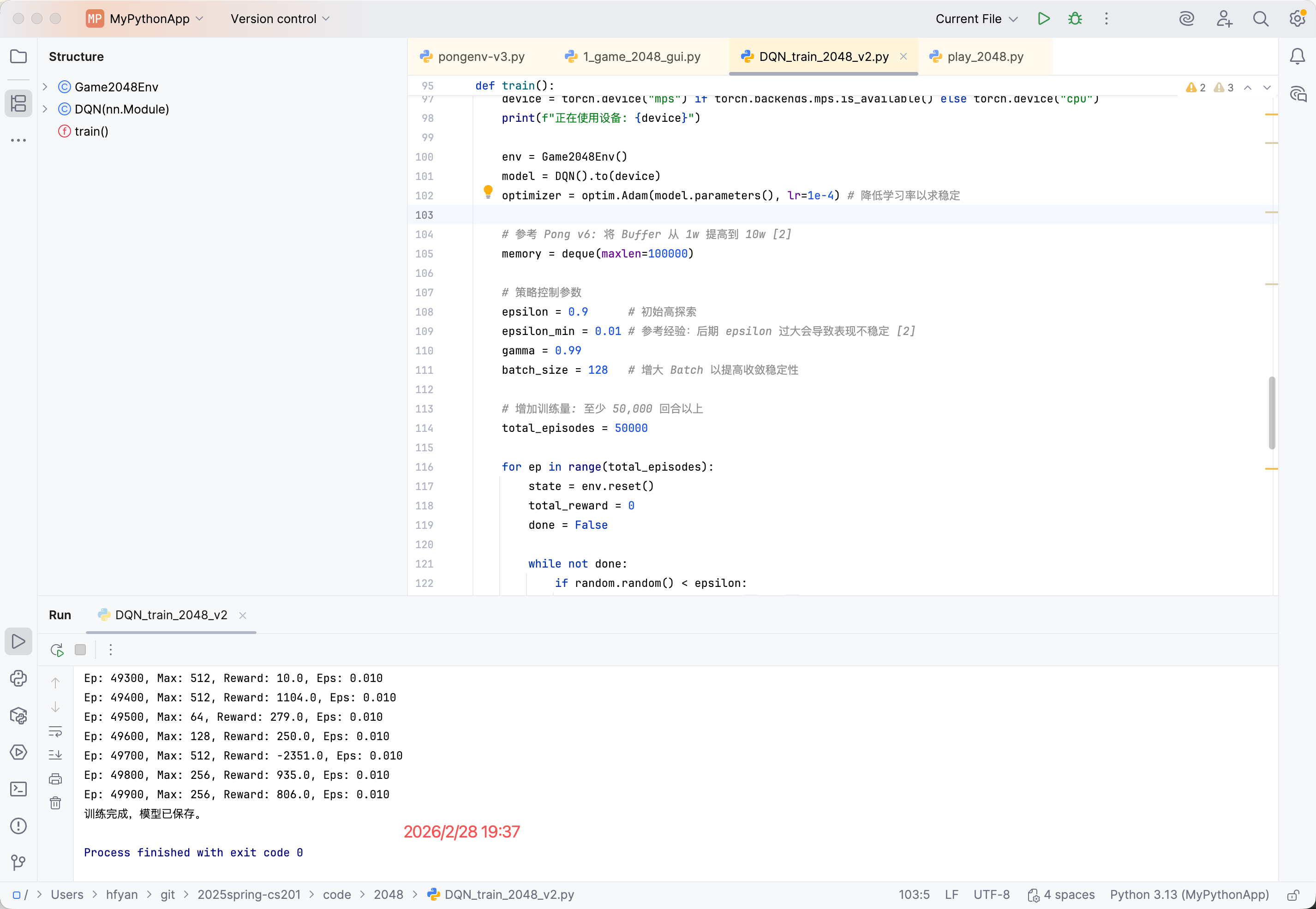
获得模型参数文件 https://github.com/GMyhf/2025spring-cs201/blob/main/code/2048/2048_bot.pth
利用模型,自动玩2048,https://github.com/GMyhf/2025spring-cs201/blob/main/code/2048/play_2048.py
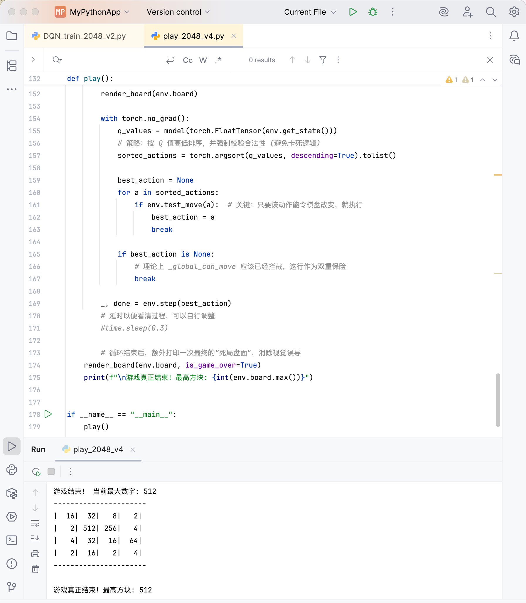
# 6. 运行《从零构建大模型》代码
《从零构建大模型》代码,https://github.com/rasbt/LLMs-from-scratch
Build a Large Language Model (From Scratch)
可以在本地 mac 或者 window 运行,配置方法方法如: ...Setup_....md。
https://github.com/GMyhf/2025fall-cs201/tree/main/LLM
附录B《大模型自我检测指南》(Test Yourself On Build a Large Language.pdf)的结构与《从零构建大语言模型》完全对应,聚焦于各章节的核心概念。可以通过多项选择题、代码与关键概念相关问题,以及需要深入思考的开放式问答题来检验自己的理解。所有题目均附有答案。
无论你当前的知识水平如何,指南都能以不同方式助你一臂之力:在阅读完某一章后使用它,可巩固所学内容;而在阅读前先浏览它,同样大有裨益——通过预先测试核心概念及其相互关系,你能更轻松地理解章节内容,并为吸收新知识做好准备。
# 附录A PyTorch教程
https://www.runoob.com/pytorch/pytorch-tutorial.html
PyTorch 是一个开源的机器学习库,主要用于进行计算机视觉(CV)、自然语言处理(NLP)、语音识别等领域的研究和开发。
PyTorch由 Facebook 的人工智能研究团队开发,并在机器学习和深度学习社区中广泛使用。
PyTorch 以其灵活性和易用性而闻名,特别适合于深度学习研究和开发。
## A.1 PyTorch安装
在已经安装好的python环境中,在terminal窗口命令行中,激活环境,并安装torch包
> Python开发环境配置指南,https://github.com/GMyhf/2025fall-cs101/blob/main/Python_Development_Setup_Mac_Windows.md
```
[hfyan@HongfeideMac-Studio MyPythonApp % source .venv/bin/activate
(.venv) hfyan@HongfeideMac-Studio MyPythonApp % uv pip install torch torchvision torchaudio
```
**验证安装**
为了确保 PyTorch 已正确安装,我们可以通过执行以下 PyTorch 代码来验证是否安装成功:
**实例**
```python
import torch
# 当前安装的 PyTorch 库的版本
print(torch.__version__)
# 检测 MPS 作为 GPU 后端是否可用(适用于 Apple Silicon)
if torch.backends.mps.is_available():
device = torch.device("mps")
print("Using MPS device for GPU acceleration")
else: # 检查 CUDA 是否可用,即你的系统有 NVIDIA 的 GPU
device = torch.device("cuda:0" if torch.cuda.is_available() else "cpu")
print("MPS device not available, using CPU")
"""
2.9.1
Using MPS device for GPU acceleration
"""
```
一个简单的实例,构建一个随机初始化的张量:
```python
import torch
x = torch.rand(5, 3)
print(x)
```
如果安装成功,输出结果类似如下:
```
tensor([[0.8622, 0.5916, 0.8073],
[0.8955, 0.7416, 0.3482],
[0.8059, 0.1414, 0.2828],
[0.0923, 0.0113, 0.4226],
[0.4438, 0.9789, 0.9048]])
```
**实例**
下面的是 PyTorch 中一些基本的张量操作:如何创建随机张量、进行逐元素运算、访问特定元素以及计算总和和最大值。
```python
import torch
# 设置数据类型和设备
dtype = torch.float # 张量数据类型为浮点型
device = torch.device("cpu") # 本次计算在 CPU 上进行
# 创建并打印两个随机张量 a 和 b
a = torch.randn(2, 3, device=device, dtype=dtype) # 创建一个 2x3 的随机张量
b = torch.randn(2, 3, device=device, dtype=dtype) # 创建另一个 2x3 的随机张量
print("张量 a:")
print(a)
print("张量 b:")
print(b)
# 逐元素相乘并输出结果
print("a 和 b 的逐元素乘积:")
print(a * b)
# 输出张量 a 所有元素的总和
print("张量 a 所有元素的总和:")
print(a.sum())
# 输出张量 a 中第 2 行第 3 列的元素(注意索引从 0 开始)
print("张量 a 第 2 行第 3 列的元素:")
print(a[1, 2])
# 输出张量 a 中的最大值
print("张量 a 中的最大值:")
print(a.max())
"""
张量 a:
tensor([[ 0.8182, 0.4718, 0.8318],
[ 0.8146, 0.1508, -1.7619]])
张量 b:
tensor([[-1.7713, 0.8521, 0.4598],
[ 0.3082, 0.0558, 0.1254]])
a 和 b 的逐元素乘积:
tensor([[-1.4493, 0.4020, 0.3824],
[ 0.2510, 0.0084, -0.2209]])
张量 a 所有元素的总和:
tensor(1.3252)
张量 a 第 2 行第 3 列的元素:
tensor(-1.7619)
张量 a 中的最大值:
tensor(0.8318)
"""
```
## A.2 PyTorch 简介
PyTorch 是一个开源的 Python 机器学习库,基于 Torch 库,底层由 C++ 实现,应用于人工智能领域,如计算机视觉和自然语言处理。
PyTorch 最初由 Meta Platforms 的人工智能研究团队开发,现在属 于Linux 基金会的一部分。
许多深度学习软件都是基于 PyTorch 构建的,包括特斯拉自动驾驶、Uber 的 Pyro、Hugging Face 的 Transformers、 PyTorch Lightning 和 Catalyst。
**PyTorch 主要有两大特征:**
- 类似于 NumPy 的张量计算,能在 GPU 或 MPS 等硬件加速器上加速。
- 基于带自动微分系统的深度神经网络。
PyTorch 包括 torch.autograd、torch.nn、torch.optim 等子模块。
PyTorch 包含多种损失函数,包括 MSE(均方误差 = L2 范数)、交叉熵损失和负熵似然损失(对分类器有用)等。
### PyTorch 特性
- **动态计算图(Dynamic Computation Graphs)**: PyTorch 的计算图是动态的,这意味着它们在运行时构建,并且可以随时改变。这为实验和调试提供了极大的灵活性,因为开发者可以逐行执行代码,查看中间结果。
- **自动微分(Automatic Differentiation)**: PyTorch 的自动微分系统允许开发者轻松地计算梯度,这对于训练深度学习模型至关重要。它通过反向传播算法自动计算出损失函数对模型参数的梯度。
- **张量计算(Tensor Computation)**: PyTorch 提供了类似于 NumPy 的张量操作,这些操作可以在 CPU 和 GPU 上执行,从而加速计算过程。张量是 PyTorch 中的基本数据结构,用于存储和操作数据。
- **丰富的 API**: PyTorch 提供了大量的预定义层、损失函数和优化算法,这些都是构建深度学习模型的常用组件。
- **多语言支持**: PyTorch 虽然以 Python 为主要接口,但也提供了 C++ 接口,允许更底层的集成和控制。
#### 动态计算图(Dynamic Computation Graph)
PyTorch 最显著的特点之一是其动态计算图的机制。
与 TensorFlow 的静态计算图(graph)不同,PyTorch 在执行时构建计算图,这意味着在每次计算时,图都会根据输入数据的形状自动变化。
**动态计算图的优点:**
- 更加灵活,特别适用于需要条件判断或递归的场景。
- 方便调试和修改,能够直接查看中间结果。
- 更接近 Python 编程的风格,易于上手。
#### 张量(Tensor)与自动求导(Autograd)
PyTorch 中的核心数据结构是 **张量(Tensor)**,它是一个多维矩阵,可以在 CPU 或 GPU 上高效地进行计算。张量的操作支持自动求导(Autograd)机制,使得在反向传播过程中自动计算梯度,这对于深度学习中的梯度下降优化算法至关重要。
**张量(Tensor):**
- 支持在 CPU 和 GPU 之间进行切换。
- 提供了类似 NumPy 的接口,支持元素级运算。
- 支持自动求导,可以方便地进行梯度计算。
**自动求导(Autograd):**
- PyTorch 内置的自动求导引擎,能够自动追踪所有张量的操作,并在反向传播时计算梯度。
- 通过 `requires_grad` 属性,可以指定张量需要计算梯度。
- 支持高效的反向传播,适用于神经网络的训练。
#### 模型定义与训练
PyTorch 提供了 `torch.nn` 模块,允许用户通过继承 `nn.Module` 类来定义神经网络模型。使用 `forward` 函数指定前向传播,自动反向传播(通过 `autograd`)和梯度计算也由 PyTorch 内部处理。
**神经网络模块(torch.nn):**
- 提供了常用的层(如线性层、卷积层、池化层等)。
- 支持定义复杂的神经网络架构(包括多输入、多输出的网络)。
- 兼容与优化器(如 `torch.optim`)一起使用。
#### GPU 加速
PyTorch 完全支持在 GPU 上运行,以加速深度学习模型的训练。通过简单的 `.to(device)` 方法,用户可以将模型和张量转移到 GPU 上进行计算。PyTorch 支持多 GPU 训练,能够利用 NVIDIA CUDA 技术显著提高计算效率。
**GPU 支持:**
- 自动选择 GPU 或 CPU。
- 支持通过 CUDA 加速运算。
- 支持多 GPU 并行计算(`DataParallel` 或 `torch.distributed`)。
#### 生态系统与社区支持
PyTorch 作为一个开源项目,拥有一个庞大的社区和生态系统。它不仅在学术界得到了广泛的应用,也在工业界,特别是在计算机视觉、自然语言处理等领域中得到了广泛部署。PyTorch 还提供了许多与深度学习相关的工具和库,如:
- **torchvision**:用于计算机视觉任务的数据集和模型。
- **torchtext**:用于自然语言处理任务的数据集和预处理工具。
- **torchaudio**:用于音频处理的工具包。
- **PyTorch Lightning**:一种简化 PyTorch 代码的高层库,专注于研究和实验的快速迭代。
------
### 与其他框架的对比
PyTorch 由于其灵活性、易用性和社区支持,已经成为很多深度学习研究者和开发者的首选框架。
#### TensorFlow vs PyTorch
- PyTorch 的动态计算图使得它更加灵活,适合快速实验和研究;而 TensorFlow 的静态计算图在生产环境中更具优化空间。
- PyTorch 在调试时更加方便,TensorFlow 则在部署上更加成熟,支持更广泛的硬件和平台。
- 近年来,TensorFlow 也引入了动态图(如 TensorFlow 2.x),使得两者在功能上趋于接近。
- 其他深度学习框架,如 Keras、Caffe 等也有一定应用,但 PyTorch 由于其灵活性、易用性和社区支持,已经成为很多深度学习研究者和开发者的首选框架。
| 特性 | **TensorFlow** | **PyTorch** |
| :----------------- | :------------------------------------------------------ | :----------------------------------------------------------- |
| **开发公司** | Google | Facebook (FAIR) |
| **计算图类型** | 静态计算图(定义后再执行) | 动态计算图(定义即执行) |
| **灵活性** | 低(计算图在编译时构建,不易修改) | 高(计算图在执行时动态创建,易于修改和调试) |
| **调试** | 较难(需要使用 `tf.debugging` 或外部工具调试) | 容易(可以直接在 Python 中进行调试) |
| **易用性** | 低(较复杂,API 较多,学习曲线较陡峭) | 高(API 简洁,语法更加接近 Python,容易上手) |
| **部署** | 强(支持广泛的硬件,如 TensorFlow Lite、TensorFlow.js) | 较弱(部署工具和平台相对较少,虽然有 TensorFlow 支持) |
| **社区支持** | 很强(成熟且庞大的社区,广泛的教程和文档) | 很强(社区活跃,特别是在学术界,快速发展的生态) |
| **模型训练** | 支持分布式训练,支持多种设备(如 CPU、GPU、TPU) | 支持分布式训练,支持多 GPU、CPU 和 TPU |
| **API 层级** | 高级API:Keras;低级API:TensorFlow Core | 高级API:TorchVision、TorchText 等;低级API:Torch |
| **性能** | 高(优化方面成熟,适合生产环境) | 高(适合研究和原型开发,生产性能也在提升) |
| **自动求导** | 通过 `tf.GradientTape` 实现动态求导(较复杂) | 通过 `autograd` 动态求导(更简洁和直观) |
| **调优与可扩展性** | 强(支持在多平台上运行,如 TensorFlow Serving 等) | 较弱(虽然在学术和实验环境中表现优越,但生产环境支持相对较少) |
| **框架灵活性** | 较低(TensorFlow 2.x 引入了动态图特性,但仍不完全灵活) | 高(动态图带来更高的灵活性) |
| **支持多种语言** | 支持多种语言(Python, C++, Java, JavaScript, etc.) | 主要支持 Python(但也有 C++ API) |
| **兼容性与迁移** | TensorFlow 2.x 与旧版本兼容性较好 | 与 TensorFlow 兼容性差,迁移较难 |
#### PyTorch vs NumPy
| 特性 | PyTorch | NumPy |
| :----------- | :----------------- | :--------------- |
| **目标** | 深度学习专用 | 通用科学计算 |
| **GPU 支持** | 原生支持 CUDA | 不直接支持 |
| **自动微分** | 内置自动求导 | 需要手动计算梯度 |
| **神经网络** | 丰富的神经网络模块 | 需要从零实现 |
| **学习成本** | 相对较高 | 相对较低 |
------
### PyTorch 的历史与发展
PyTorch 的前身是 Torch,这是一个基于 Lua 语言的科学计算框架。随着 Python 在机器学习领域的兴起,Facebook 团队决定将 Torch 的核心思想移植到 Python 上,从而诞生了 PyTorch。
- **2016年**:Facebook 发布 PyTorch 0.1 版本
- **2017年**:PyTorch 0.2 引入分布式训练支持
- **2018年**:PyTorch 1.0 发布,增加了生产部署能力
- **2019年**:PyTorch 1.3 引入移动端支持
- **2020年**:PyTorch 1.6 增加了自动混合精度训练
- **2021年**:PyTorch 1.9 引入 TorchScript 和 C++ 前端
- **2022年**:PyTorch 1.12 优化了性能和稳定性
- **2023年**:PyTorch 2.0 发布,引入编译模式大幅提升性能
## A.3 PyTorch 基础
PyTorch 是一个开源的深度学习框架,以其灵活性和动态计算图而广受欢迎。
PyTorch 主要有以下几个基础概念:张量(Tensor)、自动求导(Autograd)、神经网络模块(nn.Module)、优化器(optim)等。
- **张量(Tensor)**:PyTorch 的核心数据结构,支持多维数组,并可以在 CPU 或 GPU 上进行加速计算。
- **自动求导(Autograd)**:PyTorch 提供了自动求导功能,可以轻松计算模型的梯度,便于进行反向传播和优化。
- **神经网络(nn.Module)**:PyTorch 提供了简单且强大的 API 来构建神经网络模型,可以方便地进行前向传播和模型定义。
- **优化器(Optimizers)**:使用优化器(如 Adam、SGD 等)来更新模型的参数,使得损失最小化。
- **设备(Device)**:可以将模型和张量移动到 GPU 上以加速计算。
------
### PyTorch 架构总览
PyTorch 采用模块化设计,由多个相互协作的核心组件构成。理解这些组件的作用和相互关系,是掌握 PyTorch 的关键。
**PyTorch 架构图**
```
┌─────────────────────────────────────────────────────────────┐
│ PyTorch 生态系统 │
├─────────────────────────────────────────────────────────────┤
│ torchvision │ torchtext │ torchaudio │ 其他专业库 │
├─────────────────────────────────────────────────────────────┤
│ PyTorch 核心 │
├───────────────┬─────────────────┬───────────────────────────┤
│ torch.nn │ torch.optim │ torch.utils │
│ (神经网络) │ (优化器) │ (工具函数) │
├───────────────┼─────────────────┼───────────────────────────┤
│ │ │ torch.utils.data │
│ torch 核心 │ autograd │ (数据加载) │
│ (张量计算) │ (自动微分) │ │
└───────────────┴─────────────────┴───────────────────────────┘
```
PyTorch 采用**分层架构**设计,从上层到底层依次为:
**1、Python API(顶层)**
- `torch`:核心张量计算(类似NumPy,支持GPU)。
- `torch.nn`:神经网络层、损失函数等。
- `torch.autograd`:自动微分(反向传播)。
- 开发者直接调用的接口,简单易用。
**2、C++核心(中层)**
- **ATen**:张量运算核心库(400+操作)。
- **JIT**:即时编译优化模型。
- **Autograd引擎**:自动微分的底层实现。
- 高性能计算,连接Python与底层硬件。
**3、基础库(底层)**
- **TH/THNN**:C语言实现的基础张量和神经网络操作。
- **THC/THCUNN**:对应的CUDA(GPU)版本。
- 直接操作硬件(CPU/GPU),极致优化速度。
**执行流程**:
Python代码 → C++核心计算 → 底层CUDA/C库加速 → 返回结果。
既保持易用性,又确保高性能。
用强化学习 DQN 算法训练,在我的Mac Studio 运行19个小时。
https://github.com/GMyhf/2025spring-cs201/blob/main/code/2048/DQN_train_2048.py

获得模型参数文件 https://github.com/GMyhf/2025spring-cs201/blob/main/code/2048/2048_bot.pth
利用模型,自动玩2048,https://github.com/GMyhf/2025spring-cs201/blob/main/code/2048/play_2048.py

# 6. 运行《从零构建大模型》代码
《从零构建大模型》代码,https://github.com/rasbt/LLMs-from-scratch
Build a Large Language Model (From Scratch)
可以在本地 mac 或者 window 运行,配置方法方法如: ...Setup_....md。
https://github.com/GMyhf/2025fall-cs201/tree/main/LLM
附录B《大模型自我检测指南》(Test Yourself On Build a Large Language.pdf)的结构与《从零构建大语言模型》完全对应,聚焦于各章节的核心概念。可以通过多项选择题、代码与关键概念相关问题,以及需要深入思考的开放式问答题来检验自己的理解。所有题目均附有答案。
无论你当前的知识水平如何,指南都能以不同方式助你一臂之力:在阅读完某一章后使用它,可巩固所学内容;而在阅读前先浏览它,同样大有裨益——通过预先测试核心概念及其相互关系,你能更轻松地理解章节内容,并为吸收新知识做好准备。
# 附录A PyTorch教程
https://www.runoob.com/pytorch/pytorch-tutorial.html
PyTorch 是一个开源的机器学习库,主要用于进行计算机视觉(CV)、自然语言处理(NLP)、语音识别等领域的研究和开发。
PyTorch由 Facebook 的人工智能研究团队开发,并在机器学习和深度学习社区中广泛使用。
PyTorch 以其灵活性和易用性而闻名,特别适合于深度学习研究和开发。
## A.1 PyTorch安装
在已经安装好的python环境中,在terminal窗口命令行中,激活环境,并安装torch包
> Python开发环境配置指南,https://github.com/GMyhf/2025fall-cs101/blob/main/Python_Development_Setup_Mac_Windows.md
```
[hfyan@HongfeideMac-Studio MyPythonApp % source .venv/bin/activate
(.venv) hfyan@HongfeideMac-Studio MyPythonApp % uv pip install torch torchvision torchaudio
```
**验证安装**
为了确保 PyTorch 已正确安装,我们可以通过执行以下 PyTorch 代码来验证是否安装成功:
**实例**
```python
import torch
# 当前安装的 PyTorch 库的版本
print(torch.__version__)
# 检测 MPS 作为 GPU 后端是否可用(适用于 Apple Silicon)
if torch.backends.mps.is_available():
device = torch.device("mps")
print("Using MPS device for GPU acceleration")
else: # 检查 CUDA 是否可用,即你的系统有 NVIDIA 的 GPU
device = torch.device("cuda:0" if torch.cuda.is_available() else "cpu")
print("MPS device not available, using CPU")
"""
2.9.1
Using MPS device for GPU acceleration
"""
```
一个简单的实例,构建一个随机初始化的张量:
```python
import torch
x = torch.rand(5, 3)
print(x)
```
如果安装成功,输出结果类似如下:
```
tensor([[0.8622, 0.5916, 0.8073],
[0.8955, 0.7416, 0.3482],
[0.8059, 0.1414, 0.2828],
[0.0923, 0.0113, 0.4226],
[0.4438, 0.9789, 0.9048]])
```
**实例**
下面的是 PyTorch 中一些基本的张量操作:如何创建随机张量、进行逐元素运算、访问特定元素以及计算总和和最大值。
```python
import torch
# 设置数据类型和设备
dtype = torch.float # 张量数据类型为浮点型
device = torch.device("cpu") # 本次计算在 CPU 上进行
# 创建并打印两个随机张量 a 和 b
a = torch.randn(2, 3, device=device, dtype=dtype) # 创建一个 2x3 的随机张量
b = torch.randn(2, 3, device=device, dtype=dtype) # 创建另一个 2x3 的随机张量
print("张量 a:")
print(a)
print("张量 b:")
print(b)
# 逐元素相乘并输出结果
print("a 和 b 的逐元素乘积:")
print(a * b)
# 输出张量 a 所有元素的总和
print("张量 a 所有元素的总和:")
print(a.sum())
# 输出张量 a 中第 2 行第 3 列的元素(注意索引从 0 开始)
print("张量 a 第 2 行第 3 列的元素:")
print(a[1, 2])
# 输出张量 a 中的最大值
print("张量 a 中的最大值:")
print(a.max())
"""
张量 a:
tensor([[ 0.8182, 0.4718, 0.8318],
[ 0.8146, 0.1508, -1.7619]])
张量 b:
tensor([[-1.7713, 0.8521, 0.4598],
[ 0.3082, 0.0558, 0.1254]])
a 和 b 的逐元素乘积:
tensor([[-1.4493, 0.4020, 0.3824],
[ 0.2510, 0.0084, -0.2209]])
张量 a 所有元素的总和:
tensor(1.3252)
张量 a 第 2 行第 3 列的元素:
tensor(-1.7619)
张量 a 中的最大值:
tensor(0.8318)
"""
```
## A.2 PyTorch 简介
PyTorch 是一个开源的 Python 机器学习库,基于 Torch 库,底层由 C++ 实现,应用于人工智能领域,如计算机视觉和自然语言处理。
PyTorch 最初由 Meta Platforms 的人工智能研究团队开发,现在属 于Linux 基金会的一部分。
许多深度学习软件都是基于 PyTorch 构建的,包括特斯拉自动驾驶、Uber 的 Pyro、Hugging Face 的 Transformers、 PyTorch Lightning 和 Catalyst。
**PyTorch 主要有两大特征:**
- 类似于 NumPy 的张量计算,能在 GPU 或 MPS 等硬件加速器上加速。
- 基于带自动微分系统的深度神经网络。
PyTorch 包括 torch.autograd、torch.nn、torch.optim 等子模块。
PyTorch 包含多种损失函数,包括 MSE(均方误差 = L2 范数)、交叉熵损失和负熵似然损失(对分类器有用)等。
### PyTorch 特性
- **动态计算图(Dynamic Computation Graphs)**: PyTorch 的计算图是动态的,这意味着它们在运行时构建,并且可以随时改变。这为实验和调试提供了极大的灵活性,因为开发者可以逐行执行代码,查看中间结果。
- **自动微分(Automatic Differentiation)**: PyTorch 的自动微分系统允许开发者轻松地计算梯度,这对于训练深度学习模型至关重要。它通过反向传播算法自动计算出损失函数对模型参数的梯度。
- **张量计算(Tensor Computation)**: PyTorch 提供了类似于 NumPy 的张量操作,这些操作可以在 CPU 和 GPU 上执行,从而加速计算过程。张量是 PyTorch 中的基本数据结构,用于存储和操作数据。
- **丰富的 API**: PyTorch 提供了大量的预定义层、损失函数和优化算法,这些都是构建深度学习模型的常用组件。
- **多语言支持**: PyTorch 虽然以 Python 为主要接口,但也提供了 C++ 接口,允许更底层的集成和控制。
#### 动态计算图(Dynamic Computation Graph)
PyTorch 最显著的特点之一是其动态计算图的机制。
与 TensorFlow 的静态计算图(graph)不同,PyTorch 在执行时构建计算图,这意味着在每次计算时,图都会根据输入数据的形状自动变化。
**动态计算图的优点:**
- 更加灵活,特别适用于需要条件判断或递归的场景。
- 方便调试和修改,能够直接查看中间结果。
- 更接近 Python 编程的风格,易于上手。
#### 张量(Tensor)与自动求导(Autograd)
PyTorch 中的核心数据结构是 **张量(Tensor)**,它是一个多维矩阵,可以在 CPU 或 GPU 上高效地进行计算。张量的操作支持自动求导(Autograd)机制,使得在反向传播过程中自动计算梯度,这对于深度学习中的梯度下降优化算法至关重要。
**张量(Tensor):**
- 支持在 CPU 和 GPU 之间进行切换。
- 提供了类似 NumPy 的接口,支持元素级运算。
- 支持自动求导,可以方便地进行梯度计算。
**自动求导(Autograd):**
- PyTorch 内置的自动求导引擎,能够自动追踪所有张量的操作,并在反向传播时计算梯度。
- 通过 `requires_grad` 属性,可以指定张量需要计算梯度。
- 支持高效的反向传播,适用于神经网络的训练。
#### 模型定义与训练
PyTorch 提供了 `torch.nn` 模块,允许用户通过继承 `nn.Module` 类来定义神经网络模型。使用 `forward` 函数指定前向传播,自动反向传播(通过 `autograd`)和梯度计算也由 PyTorch 内部处理。
**神经网络模块(torch.nn):**
- 提供了常用的层(如线性层、卷积层、池化层等)。
- 支持定义复杂的神经网络架构(包括多输入、多输出的网络)。
- 兼容与优化器(如 `torch.optim`)一起使用。
#### GPU 加速
PyTorch 完全支持在 GPU 上运行,以加速深度学习模型的训练。通过简单的 `.to(device)` 方法,用户可以将模型和张量转移到 GPU 上进行计算。PyTorch 支持多 GPU 训练,能够利用 NVIDIA CUDA 技术显著提高计算效率。
**GPU 支持:**
- 自动选择 GPU 或 CPU。
- 支持通过 CUDA 加速运算。
- 支持多 GPU 并行计算(`DataParallel` 或 `torch.distributed`)。
#### 生态系统与社区支持
PyTorch 作为一个开源项目,拥有一个庞大的社区和生态系统。它不仅在学术界得到了广泛的应用,也在工业界,特别是在计算机视觉、自然语言处理等领域中得到了广泛部署。PyTorch 还提供了许多与深度学习相关的工具和库,如:
- **torchvision**:用于计算机视觉任务的数据集和模型。
- **torchtext**:用于自然语言处理任务的数据集和预处理工具。
- **torchaudio**:用于音频处理的工具包。
- **PyTorch Lightning**:一种简化 PyTorch 代码的高层库,专注于研究和实验的快速迭代。
------
### 与其他框架的对比
PyTorch 由于其灵活性、易用性和社区支持,已经成为很多深度学习研究者和开发者的首选框架。
#### TensorFlow vs PyTorch
- PyTorch 的动态计算图使得它更加灵活,适合快速实验和研究;而 TensorFlow 的静态计算图在生产环境中更具优化空间。
- PyTorch 在调试时更加方便,TensorFlow 则在部署上更加成熟,支持更广泛的硬件和平台。
- 近年来,TensorFlow 也引入了动态图(如 TensorFlow 2.x),使得两者在功能上趋于接近。
- 其他深度学习框架,如 Keras、Caffe 等也有一定应用,但 PyTorch 由于其灵活性、易用性和社区支持,已经成为很多深度学习研究者和开发者的首选框架。
| 特性 | **TensorFlow** | **PyTorch** |
| :----------------- | :------------------------------------------------------ | :----------------------------------------------------------- |
| **开发公司** | Google | Facebook (FAIR) |
| **计算图类型** | 静态计算图(定义后再执行) | 动态计算图(定义即执行) |
| **灵活性** | 低(计算图在编译时构建,不易修改) | 高(计算图在执行时动态创建,易于修改和调试) |
| **调试** | 较难(需要使用 `tf.debugging` 或外部工具调试) | 容易(可以直接在 Python 中进行调试) |
| **易用性** | 低(较复杂,API 较多,学习曲线较陡峭) | 高(API 简洁,语法更加接近 Python,容易上手) |
| **部署** | 强(支持广泛的硬件,如 TensorFlow Lite、TensorFlow.js) | 较弱(部署工具和平台相对较少,虽然有 TensorFlow 支持) |
| **社区支持** | 很强(成熟且庞大的社区,广泛的教程和文档) | 很强(社区活跃,特别是在学术界,快速发展的生态) |
| **模型训练** | 支持分布式训练,支持多种设备(如 CPU、GPU、TPU) | 支持分布式训练,支持多 GPU、CPU 和 TPU |
| **API 层级** | 高级API:Keras;低级API:TensorFlow Core | 高级API:TorchVision、TorchText 等;低级API:Torch |
| **性能** | 高(优化方面成熟,适合生产环境) | 高(适合研究和原型开发,生产性能也在提升) |
| **自动求导** | 通过 `tf.GradientTape` 实现动态求导(较复杂) | 通过 `autograd` 动态求导(更简洁和直观) |
| **调优与可扩展性** | 强(支持在多平台上运行,如 TensorFlow Serving 等) | 较弱(虽然在学术和实验环境中表现优越,但生产环境支持相对较少) |
| **框架灵活性** | 较低(TensorFlow 2.x 引入了动态图特性,但仍不完全灵活) | 高(动态图带来更高的灵活性) |
| **支持多种语言** | 支持多种语言(Python, C++, Java, JavaScript, etc.) | 主要支持 Python(但也有 C++ API) |
| **兼容性与迁移** | TensorFlow 2.x 与旧版本兼容性较好 | 与 TensorFlow 兼容性差,迁移较难 |
#### PyTorch vs NumPy
| 特性 | PyTorch | NumPy |
| :----------- | :----------------- | :--------------- |
| **目标** | 深度学习专用 | 通用科学计算 |
| **GPU 支持** | 原生支持 CUDA | 不直接支持 |
| **自动微分** | 内置自动求导 | 需要手动计算梯度 |
| **神经网络** | 丰富的神经网络模块 | 需要从零实现 |
| **学习成本** | 相对较高 | 相对较低 |
------
### PyTorch 的历史与发展
PyTorch 的前身是 Torch,这是一个基于 Lua 语言的科学计算框架。随着 Python 在机器学习领域的兴起,Facebook 团队决定将 Torch 的核心思想移植到 Python 上,从而诞生了 PyTorch。
- **2016年**:Facebook 发布 PyTorch 0.1 版本
- **2017年**:PyTorch 0.2 引入分布式训练支持
- **2018年**:PyTorch 1.0 发布,增加了生产部署能力
- **2019年**:PyTorch 1.3 引入移动端支持
- **2020年**:PyTorch 1.6 增加了自动混合精度训练
- **2021年**:PyTorch 1.9 引入 TorchScript 和 C++ 前端
- **2022年**:PyTorch 1.12 优化了性能和稳定性
- **2023年**:PyTorch 2.0 发布,引入编译模式大幅提升性能
## A.3 PyTorch 基础
PyTorch 是一个开源的深度学习框架,以其灵活性和动态计算图而广受欢迎。
PyTorch 主要有以下几个基础概念:张量(Tensor)、自动求导(Autograd)、神经网络模块(nn.Module)、优化器(optim)等。
- **张量(Tensor)**:PyTorch 的核心数据结构,支持多维数组,并可以在 CPU 或 GPU 上进行加速计算。
- **自动求导(Autograd)**:PyTorch 提供了自动求导功能,可以轻松计算模型的梯度,便于进行反向传播和优化。
- **神经网络(nn.Module)**:PyTorch 提供了简单且强大的 API 来构建神经网络模型,可以方便地进行前向传播和模型定义。
- **优化器(Optimizers)**:使用优化器(如 Adam、SGD 等)来更新模型的参数,使得损失最小化。
- **设备(Device)**:可以将模型和张量移动到 GPU 上以加速计算。
------
### PyTorch 架构总览
PyTorch 采用模块化设计,由多个相互协作的核心组件构成。理解这些组件的作用和相互关系,是掌握 PyTorch 的关键。
**PyTorch 架构图**
```
┌─────────────────────────────────────────────────────────────┐
│ PyTorch 生态系统 │
├─────────────────────────────────────────────────────────────┤
│ torchvision │ torchtext │ torchaudio │ 其他专业库 │
├─────────────────────────────────────────────────────────────┤
│ PyTorch 核心 │
├───────────────┬─────────────────┬───────────────────────────┤
│ torch.nn │ torch.optim │ torch.utils │
│ (神经网络) │ (优化器) │ (工具函数) │
├───────────────┼─────────────────┼───────────────────────────┤
│ │ │ torch.utils.data │
│ torch 核心 │ autograd │ (数据加载) │
│ (张量计算) │ (自动微分) │ │
└───────────────┴─────────────────┴───────────────────────────┘
```
PyTorch 采用**分层架构**设计,从上层到底层依次为:
**1、Python API(顶层)**
- `torch`:核心张量计算(类似NumPy,支持GPU)。
- `torch.nn`:神经网络层、损失函数等。
- `torch.autograd`:自动微分(反向传播)。
- 开发者直接调用的接口,简单易用。
**2、C++核心(中层)**
- **ATen**:张量运算核心库(400+操作)。
- **JIT**:即时编译优化模型。
- **Autograd引擎**:自动微分的底层实现。
- 高性能计算,连接Python与底层硬件。
**3、基础库(底层)**
- **TH/THNN**:C语言实现的基础张量和神经网络操作。
- **THC/THCUNN**:对应的CUDA(GPU)版本。
- 直接操作硬件(CPU/GPU),极致优化速度。
**执行流程**:
Python代码 → C++核心计算 → 底层CUDA/C库加速 → 返回结果。
既保持易用性,又确保高性能。
 **张量(Tensor)**
张量(Tensor)是 PyTorch 中的核心数据结构,用于存储和操作多维数组。
张量可以视为一个多维数组,支持加速计算的操作。
在 PyTorch 中,张量的概念类似于 NumPy 中的数组,但是 PyTorch 的张量可以运行在不同的设备上,比如 CPU 和 GPU,这使得它们非常适合于进行大规模并行计算,特别是在深度学习领域。
- **维度(Dimensionality)**:张量的维度指的是数据的多维数组结构。例如,一个标量(0维张量)是一个单独的数字,一个向量(1维张量)是一个一维数组,一个矩阵(2维张量)是一个二维数组,以此类推。
- **形状(Shape)**:张量的形状是指每个维度上的大小。例如,一个形状为`(3, 4)`的张量意味着它有3行4列。
- **数据类型(Dtype)**:张量中的数据类型定义了存储每个元素所需的内存大小和解释方式。PyTorch支持多种数据类型,包括整数型(如`torch.int8`、`torch.int32`)、浮点型(如`torch.float32`、`torch.float64`)和布尔型(`torch.bool`)。
**张量创建:**
**实例**
```python
import torch
# 创建一个 2x3 的全 0 张量
a = torch.zeros(2, 3)
print(a)
# 创建一个 2x3 的全 1 张量
b = torch.ones(2, 3)
print(b)
# 创建一个 2x3 的随机数张量
c = torch.randn(2, 3)
print(c)
# 从 NumPy 数组创建张量
import numpy as np
numpy_array = np.array([[1, 2], [3, 4]])
tensor_from_numpy = torch.from_numpy(numpy_array)
print(tensor_from_numpy)
# 在指定设备(CPU/GPU)上创建张量
device = torch.device("cuda" if torch.cuda.is_available() else "cpu")
d = torch.randn(2, 3, device=device)
print(d)
```
输出结果类似如下:
```
tensor([[0., 0., 0.],
[0., 0., 0.]])
tensor([[1., 1., 1.],
[1., 1., 1.]])
tensor([[ 1.0189, -0.5718, -1.2814],
[-0.5865, 1.0855, 1.1727]])
tensor([[1, 2],
[3, 4]])
tensor([[-0.3360, 0.2203, 1.3463],
[-0.5982, -0.2704, 0.5429]])
```
**常用张量操作:**
**实例**
```py
# 张量相加
e = torch.randn(2, 3)
f = torch.randn(2, 3)
print(e + f)
# 逐元素乘法
print(e * f)
# 张量的转置
g = torch.randn(3, 2)
print(g.t()) # 或者 g.transpose(0, 1)
# 张量的形状
print(g.shape) # 返回形状
```
**张量与设备**
PyTorch 张量可以存在于不同的设备上,包括CPU和GPU,你可以将张量移动到 GPU 上以加速计算:
```
if torch.cuda.is_available():
tensor_gpu = tensor_from_list.to('cuda') # 将张量移动到GPU
```
**梯度和自动微分**
PyTorch的张量支持自动微分,这是深度学习中的关键特性。当你创建一个需要梯度的张量时,PyTorch可以自动计算其梯度:
**实例**
```python
# 创建一个需要梯度的张量
tensor_requires_grad = torch.tensor([1.0], requires_grad=True)
# 进行一些操作
tensor_result = tensor_requires_grad * 2
# 计算梯度
tensor_result.backward()
print(tensor_requires_grad.grad) # 输出梯度
```
**内存和性能**
PyTorch 张量还提供了一些内存管理功能,比如.clone()、.detach() 和 .to() 方法,它们可以帮助你优化内存使用和提高性能。
------
### 自动求导(Autograd)
自动求导(Automatic Differentiation,简称Autograd)是深度学习框架中的一个核心特性,它允许计算机自动计算数学函数的导数。
在深度学习中,自动求导主要用于两个方面:**一是在训练神经网络时计算梯度**,**二是进行反向传播算法的实现**。
自动求导基于链式法则(Chain Rule),这是一个用于计算复杂函数导数的数学法则。链式法则表明,复合函数的导数是其各个组成部分导数的乘积。在深度学习中,模型通常是由许多层组成的复杂函数,自动求导能够高效地计算这些层的梯度。
**动态图与静态图:**
- **动态图(Dynamic Graph)**:在动态图中,计算图在运行时动态构建。每次执行操作时,计算图都会更新,这使得调试和修改模型变得更加容易。PyTorch使用的是动态图。
- **静态图(Static Graph)**:在静态图中,计算图在开始执行之前构建完成,并且不会改变。TensorFlow最初使用的是静态图,但后来也支持动态图。
PyTorch 提供了自动求导功能,通过 autograd 模块来自动计算梯度。
torch.Tensor 对象有一个 requires_grad 属性,用于指示是否需要计算该张量的梯度。
当你创建一个 requires_grad=True 的张量时,PyTorch 会自动跟踪所有对它的操作,以便在之后计算梯度。
创建需要梯度的张量:
**实例**
```python
# 创建一个需要计算梯度的张量
x = torch.randn(2, 2, requires_grad=True)
print(x)
# 执行某些操作
y = x + 2
z = y * y * 3
out = z.mean()
print(out)
```
输出结果类似如下:
```
tensor([[0., 0., 0.],
[0., 0., 0.]])
tensor([[1., 1., 1.],
[1., 1., 1.]])
tensor([[ 1.0189, -0.5718, -1.2814],
[-0.5865, 1.0855, 1.1727]])
tensor([[1, 2],
[3, 4]])
tensor([[-0.3360, 0.2203, 1.3463],
[-0.5982, -0.2704, 0.5429]])
tianqixin@Mac-mini runoob-test % python3 test.py
tensor([[-0.1908, 0.2811],
[ 0.8068, 0.8002]], requires_grad=True)
tensor(18.1469, grad_fn=
**张量(Tensor)**
张量(Tensor)是 PyTorch 中的核心数据结构,用于存储和操作多维数组。
张量可以视为一个多维数组,支持加速计算的操作。
在 PyTorch 中,张量的概念类似于 NumPy 中的数组,但是 PyTorch 的张量可以运行在不同的设备上,比如 CPU 和 GPU,这使得它们非常适合于进行大规模并行计算,特别是在深度学习领域。
- **维度(Dimensionality)**:张量的维度指的是数据的多维数组结构。例如,一个标量(0维张量)是一个单独的数字,一个向量(1维张量)是一个一维数组,一个矩阵(2维张量)是一个二维数组,以此类推。
- **形状(Shape)**:张量的形状是指每个维度上的大小。例如,一个形状为`(3, 4)`的张量意味着它有3行4列。
- **数据类型(Dtype)**:张量中的数据类型定义了存储每个元素所需的内存大小和解释方式。PyTorch支持多种数据类型,包括整数型(如`torch.int8`、`torch.int32`)、浮点型(如`torch.float32`、`torch.float64`)和布尔型(`torch.bool`)。
**张量创建:**
**实例**
```python
import torch
# 创建一个 2x3 的全 0 张量
a = torch.zeros(2, 3)
print(a)
# 创建一个 2x3 的全 1 张量
b = torch.ones(2, 3)
print(b)
# 创建一个 2x3 的随机数张量
c = torch.randn(2, 3)
print(c)
# 从 NumPy 数组创建张量
import numpy as np
numpy_array = np.array([[1, 2], [3, 4]])
tensor_from_numpy = torch.from_numpy(numpy_array)
print(tensor_from_numpy)
# 在指定设备(CPU/GPU)上创建张量
device = torch.device("cuda" if torch.cuda.is_available() else "cpu")
d = torch.randn(2, 3, device=device)
print(d)
```
输出结果类似如下:
```
tensor([[0., 0., 0.],
[0., 0., 0.]])
tensor([[1., 1., 1.],
[1., 1., 1.]])
tensor([[ 1.0189, -0.5718, -1.2814],
[-0.5865, 1.0855, 1.1727]])
tensor([[1, 2],
[3, 4]])
tensor([[-0.3360, 0.2203, 1.3463],
[-0.5982, -0.2704, 0.5429]])
```
**常用张量操作:**
**实例**
```py
# 张量相加
e = torch.randn(2, 3)
f = torch.randn(2, 3)
print(e + f)
# 逐元素乘法
print(e * f)
# 张量的转置
g = torch.randn(3, 2)
print(g.t()) # 或者 g.transpose(0, 1)
# 张量的形状
print(g.shape) # 返回形状
```
**张量与设备**
PyTorch 张量可以存在于不同的设备上,包括CPU和GPU,你可以将张量移动到 GPU 上以加速计算:
```
if torch.cuda.is_available():
tensor_gpu = tensor_from_list.to('cuda') # 将张量移动到GPU
```
**梯度和自动微分**
PyTorch的张量支持自动微分,这是深度学习中的关键特性。当你创建一个需要梯度的张量时,PyTorch可以自动计算其梯度:
**实例**
```python
# 创建一个需要梯度的张量
tensor_requires_grad = torch.tensor([1.0], requires_grad=True)
# 进行一些操作
tensor_result = tensor_requires_grad * 2
# 计算梯度
tensor_result.backward()
print(tensor_requires_grad.grad) # 输出梯度
```
**内存和性能**
PyTorch 张量还提供了一些内存管理功能,比如.clone()、.detach() 和 .to() 方法,它们可以帮助你优化内存使用和提高性能。
------
### 自动求导(Autograd)
自动求导(Automatic Differentiation,简称Autograd)是深度学习框架中的一个核心特性,它允许计算机自动计算数学函数的导数。
在深度学习中,自动求导主要用于两个方面:**一是在训练神经网络时计算梯度**,**二是进行反向传播算法的实现**。
自动求导基于链式法则(Chain Rule),这是一个用于计算复杂函数导数的数学法则。链式法则表明,复合函数的导数是其各个组成部分导数的乘积。在深度学习中,模型通常是由许多层组成的复杂函数,自动求导能够高效地计算这些层的梯度。
**动态图与静态图:**
- **动态图(Dynamic Graph)**:在动态图中,计算图在运行时动态构建。每次执行操作时,计算图都会更新,这使得调试和修改模型变得更加容易。PyTorch使用的是动态图。
- **静态图(Static Graph)**:在静态图中,计算图在开始执行之前构建完成,并且不会改变。TensorFlow最初使用的是静态图,但后来也支持动态图。
PyTorch 提供了自动求导功能,通过 autograd 模块来自动计算梯度。
torch.Tensor 对象有一个 requires_grad 属性,用于指示是否需要计算该张量的梯度。
当你创建一个 requires_grad=True 的张量时,PyTorch 会自动跟踪所有对它的操作,以便在之后计算梯度。
创建需要梯度的张量:
**实例**
```python
# 创建一个需要计算梯度的张量
x = torch.randn(2, 2, requires_grad=True)
print(x)
# 执行某些操作
y = x + 2
z = y * y * 3
out = z.mean()
print(out)
```
输出结果类似如下:
```
tensor([[0., 0., 0.],
[0., 0., 0.]])
tensor([[1., 1., 1.],
[1., 1., 1.]])
tensor([[ 1.0189, -0.5718, -1.2814],
[-0.5865, 1.0855, 1.1727]])
tensor([[1, 2],
[3, 4]])
tensor([[-0.3360, 0.2203, 1.3463],
[-0.5982, -0.2704, 0.5429]])
tianqixin@Mac-mini runoob-test % python3 test.py
tensor([[-0.1908, 0.2811],
[ 0.8068, 0.8002]], requires_grad=True)
tensor(18.1469, grad_fn= 这里,**wj** 是权重,**xj** 是输入,而 **Bias** 是偏置项。
**层(Layer)**
输入层和输出层之间的层被称为隐藏层,层与层之间的连接密度和类型构成了网络的配置。
神经网络由多个层组成,包括:
- **输入层(Input Layer)**:接收原始输入数据。
- **隐藏层(Hidden Layer)**:对输入数据进行处理,可以有多个隐藏层。
- **输出层(Output Layer)**:产生最终的输出结果。
典型的神经网络架构:
这里,**wj** 是权重,**xj** 是输入,而 **Bias** 是偏置项。
**层(Layer)**
输入层和输出层之间的层被称为隐藏层,层与层之间的连接密度和类型构成了网络的配置。
神经网络由多个层组成,包括:
- **输入层(Input Layer)**:接收原始输入数据。
- **隐藏层(Hidden Layer)**:对输入数据进行处理,可以有多个隐藏层。
- **输出层(Output Layer)**:产生最终的输出结果。
典型的神经网络架构:
 **前馈神经网络(Feedforward Neural Network,FNN)**
前馈神经网络(Feedforward Neural Network,FNN)是神经网络家族中的基本单元。
前馈神经网络特点是数据从输入层开始,经过一个或多个隐藏层,最后到达输出层,全过程没有循环或反馈。
**前馈神经网络的基本结构:**
- **输入层:** 数据进入网络的入口点。输入层的每个节点代表一个输入特征。
- **隐藏层:**一个或多个层,用于捕获数据的非线性特征。每个隐藏层由多个神经元组成,每个神经元通过激活函数增加非线性能力。
- **输出层:**输出网络的预测结果。节点数和问题类型相关,例如分类问题的输出节点数等于类别数。
- **连接权重与偏置:**每个神经元的输入通过权重进行加权求和,并加上偏置值,然后通过激活函数传递。
**循环神经网络(Recurrent Neural Network, RNN)**
循环神经网络(Recurrent Neural Network, RNN)络是一类专门处理序列数据的神经网络,能够捕获输入数据中时间或顺序信息的依赖关系。
RNN 的特别之处在于它具有"记忆能力",可以在网络的隐藏状态中保存之前时间步的信息。
循环神经网络用于处理随时间变化的数据模式。
在 RNN 中,相同的层被用来接收输入参数,并在指定的神经网络中显示输出参数。
**前馈神经网络(Feedforward Neural Network,FNN)**
前馈神经网络(Feedforward Neural Network,FNN)是神经网络家族中的基本单元。
前馈神经网络特点是数据从输入层开始,经过一个或多个隐藏层,最后到达输出层,全过程没有循环或反馈。

**前馈神经网络的基本结构:**
- **输入层:** 数据进入网络的入口点。输入层的每个节点代表一个输入特征。
- **隐藏层:**一个或多个层,用于捕获数据的非线性特征。每个隐藏层由多个神经元组成,每个神经元通过激活函数增加非线性能力。
- **输出层:**输出网络的预测结果。节点数和问题类型相关,例如分类问题的输出节点数等于类别数。
- **连接权重与偏置:**每个神经元的输入通过权重进行加权求和,并加上偏置值,然后通过激活函数传递。
**循环神经网络(Recurrent Neural Network, RNN)**
循环神经网络(Recurrent Neural Network, RNN)络是一类专门处理序列数据的神经网络,能够捕获输入数据中时间或顺序信息的依赖关系。
RNN 的特别之处在于它具有"记忆能力",可以在网络的隐藏状态中保存之前时间步的信息。
循环神经网络用于处理随时间变化的数据模式。
在 RNN 中,相同的层被用来接收输入参数,并在指定的神经网络中显示输出参数。
 PyTorch 提供了强大的工具来构建和训练神经网络。
神经网络在 PyTorch 中是通过 **torch.nn** 模块来实现的。
**torch.nn** 模块提供了各种网络层(如全连接层、卷积层等)、损失函数和优化器,让神经网络的构建和训练变得更加方便。
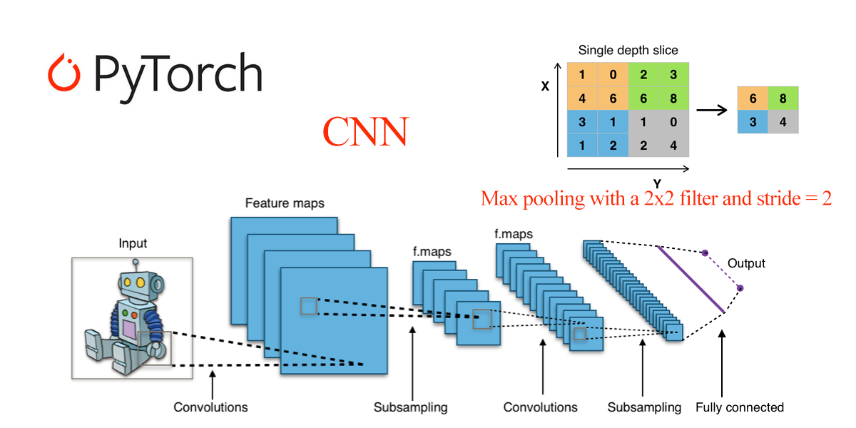
在 PyTorch 中,构建神经网络通常需要继承 nn.Module 类。
nn.Module 是所有神经网络模块的基类,你需要定义以下两个部分:
- **`__init__()`**:定义网络层。
- **`forward()`**:定义数据的前向传播过程。
简单的全连接神经网络(Fully Connected Network):
**实例**
```python
import torch
import torch.nn as nn
# 定义一个简单的神经网络模型
class SimpleNN(nn.Module):
def init(self):
super(SimpleNN, self).init()
# 定义一个输入层到隐藏层的全连接层
self.fc1 = nn.Linear(2, 2) # 输入 2 个特征,输出 2 个特征
# 定义一个隐藏层到输出层的全连接层
self.fc2 = nn.Linear(2, 1) # 输入 2 个特征,输出 1 个预测值
def forward(self, x):
# 前向传播过程
x = torch.relu(self.fc1(x)) # 使用 ReLU 激活函数
x = self.fc2(x) # 输出层
return x
# 创建模型实例
model = SimpleNN()
# 打印模型
print(model)
```
输出结果如下:
```
SimpleNN(
(fc1): Linear(in_features=2, out_features=2, bias=True)
(fc2): Linear(in_features=2, out_features=1, bias=True)
)
```
PyTorch 提供了许多常见的神经网络层,以下是几个常见的:
- **`nn.Linear(in_features, out_features)`**:全连接层,输入 `in_features` 个特征,输出 `out_features` 个特征。
- **`nn.Conv2d(in_channels, out_channels, kernel_size)`**:2D 卷积层,用于图像处理。
- **`nn.MaxPool2d(kernel_size)`**:2D 最大池化层,用于降维。
- **`nn.ReLU()`**:ReLU 激活函数,常用于隐藏层。
- **`nn.Softmax(dim)`**:Softmax 激活函数,通常用于输出层,适用于多类分类问题。
**激活函数(Activation Function)**
激活函数决定了神经元是否应该被激活。它们是非线性函数,使得神经网络能够学习和执行更复杂的任务。常见的激活函数包括:
- Sigmoid:用于二分类问题,输出值在 0 和 1 之间。
- Tanh:输出值在 -1 和 1 之间,常用于输出层之前。
- ReLU(Rectified Linear Unit):目前最流行的激活函数之一,定义为 `f(x) = max(0, x)`,有助于解决梯度消失问题。
- Softmax:常用于多分类问题的输出层,将输出转换为概率分布。
**实例**
```python
import torch.nn.functional as F
# ReLU 激活
output = F.relu(input_tensor)
# Sigmoid 激活
output = torch.sigmoid(input_tensor)
# Tanh 激活
output = torch.tanh(input_tensor)
```
**损失函数(Loss Function)**
损失函数用于衡量模型的预测值与真实值之间的差异。
常见的损失函数包括:
- **均方误差(MSELoss)**:回归问题常用,计算输出与目标值的平方差。
- **交叉熵损失(CrossEntropyLoss)**:分类问题常用,计算输出和真实标签之间的交叉熵。
- **BCEWithLogitsLoss**:二分类问题,结合了 Sigmoid 激活和二元交叉熵损失。
**实例**
```python
# 均方误差损失
criterion = nn.MSELoss()
# 交叉熵损失
criterion = nn.CrossEntropyLoss()
# 二分类交叉熵损失
criterion = nn.BCEWithLogitsLoss()
```
**优化器(Optimizer)**
优化器负责在训练过程中更新网络的权重和偏置。
常见的优化器包括:
- SGD(随机梯度下降)
- Adam(自适应矩估计)
- RMSprop(均方根传播)
**实例**
```python
import torch.optim as optim
# 使用 SGD 优化器
optimizer = optim.SGD(model.parameters(), lr=0.01)
# 使用 Adam 优化器
optimizer = optim.Adam(model.parameters(), lr=0.001)
```
**训练过程(Training Process)**
训练神经网络涉及以下步骤:
1. **准备数据**:通过 `DataLoader` 加载数据。
2. **定义损失函数和优化器**。
3. **前向传播**:计算模型的输出。
4. **计算损失**:与目标进行比较,得到损失值。
5. **反向传播**:通过 `loss.backward()` 计算梯度。
6. **更新参数**:通过 `optimizer.step()` 更新模型的参数。
7. **重复上述步骤**,直到达到预定的训练轮数。
**实例**
```python
\# 假设已经定义好了模型、损失函数和优化器
\# 训练数据示例
X = torch.randn(10, 2) # 10 个样本,每个样本有 2 个特征
Y = torch.randn(10, 1) # 10 个目标标签
\# 训练过程
for epoch in range(100): # 训练 100 轮
model.train() # 设置模型为训练模式
optimizer.zero_grad() # 清除梯度
output = model(X) # 前向传播
loss = criterion(output, Y) # 计算损失
loss.backward() # 反向传播
optimizer.step() # 更新权重
if (epoch + 1) % 10 == 0: # 每 10 轮输出一次损失
print(f'Epoch [{epoch + 1}/100], Loss: {loss.item():.4f}')
```
**测试与评估**
训练完成后,需要对模型进行测试和评估。
常见的步骤包括:
- **计算测试集的损失**:测试模型在未见过的数据上的表现。
- **计算准确率(Accuracy)**:对于分类问题,计算正确预测的比例。
**实例**
```python
# 假设你有测试集 X_test 和 Y_test
model.eval() # 设置模型为评估模式
with torch.no_grad(): # 在评估过程中禁用梯度计算
output = model(X_test)
loss = criterion(output, Y_test)
print(f'Test Loss: {loss.item():.4f}')
```
**神经网络类型**
1. **前馈神经网络(Feedforward Neural Networks)**:数据单向流动,从输入层到输出层,无反馈连接。
2. **卷积神经网络(Convolutional Neural Networks, CNNs)**:适用于图像处理,使用卷积层提取空间特征。
3. **循环神经网络(Recurrent Neural Networks, RNNs)**:适用于序列数据,如时间序列分析和自然语言处理,允许信息反馈循环。
4. **长短期记忆网络(Long Short-Term Memory, LSTM)**:一种特殊的RNN,能够学习长期依赖关系。
## A.6 PyTorch 第一个神经网络
本章节我们将介绍如何用 PyTorch 实现一个简单的前馈神经网络,完成一个二分类任务。
以下实例展示了如何使用 PyTorch 实现一个简单的神经网络进行二分类任务训练。
网络结构包括输入层、隐藏层和输出层,使用了 ReLU 激活函数和 Sigmoid 激活函数。
采用了均方误差损失函数和随机梯度下降优化器。
训练过程是通过前向传播、计算损失、反向传播和参数更新来逐步调整模型参数。
**实例**
```python
# 导入PyTorch库
import torch
import torch.nn as nn
# 定义输入层大小、隐藏层大小、输出层大小和批量大小
n_in, n_h, n_out, batch_size = 10, 5, 1, 10
# 创建虚拟输入数据和目标数据
x = torch.randn(batch_size, n_in) # 随机生成输入数据
y = torch.tensor([[1.0], [0.0], [0.0],
[1.0], [1.0], [1.0], [0.0], [0.0], [1.0], [1.0]]) # 目标输出数据
# 创建顺序模型,包含线性层、ReLU激活函数和Sigmoid激活函数
model = nn.Sequential(
nn.Linear(n_in, n_h), # 输入层到隐藏层的线性变换
nn.ReLU(), # 隐藏层的ReLU激活函数
nn.Linear(n_h, n_out), # 隐藏层到输出层的线性变换
nn.Sigmoid() # 输出层的Sigmoid激活函数
)
# 定义均方误差损失函数和随机梯度下降优化器
criterion = torch.nn.MSELoss()
optimizer = torch.optim.SGD(model.parameters(), lr=0.01) # 学习率为0.01
# 执行梯度下降算法进行模型训练
for epoch in range(50): # 迭代50次
y_pred = model(x) # 前向传播,计算预测值
loss = criterion(y_pred, y) # 计算损失
print('epoch: ', epoch, 'loss: ', loss.item()) # 打印损失值
optimizer.zero_grad() # 清零梯度
loss.backward() # 反向传播,计算梯度
optimizer.step() # 更新模型参数
```
输出结果类似如下:
```
epoch: 0 loss: 0.2302265167236328
epoch: 1 loss: 0.23012931644916534
epoch: 2 loss: 0.23003216087818146
epoch: 3 loss: 0.22993502020835876
epoch: 4 loss: 0.22983793914318085
...
```
定义网络参数:
```
n_in, n_h, n_out, batch_size = 10, 5, 1, 10
```
- `n_in`:输入层大小为 10,即每个数据点有 10 个特征。
- `n_h`:隐藏层大小为 5,即隐藏层包含 5 个神经元。
- `n_out`:输出层大小为 1,即输出一个标量,表示二分类结果(0 或 1)。
- `batch_size`:每个批次包含 10 个样本。
生成输入数据和目标数据:
```python
x = torch.randn(batch_size, n_in) # 随机生成输入数据
y = torch.tensor([[1.0], [0.0], [0.0],
[1.0], [1.0], [1.0], [0.0], [0.0], [1.0], [1.0]]) # 目标输出数据
```
- `x`:随机生成一个形状为 `(10, 10)` 的输入数据矩阵,表示 10 个样本,每个样本有 10 个特征。
- `y`:目标输出数据(标签),表示每个输入样本的类别标签(0 或 1),是一个 10×1 的张量。
定义神经网络模型:
```python
model = nn.Sequential(
nn.Linear(n_in, n_h), # 输入层到隐藏层的线性变换
nn.ReLU(), # 隐藏层的ReLU激活函数
nn.Linear(n_h, n_out), # 隐藏层到输出层的线性变换
nn.Sigmoid() # 输出层的Sigmoid激活函数
)
```
`nn.Sequential` 用于按顺序定义网络层。
- `nn.Linear(n_in, n_h)`:定义输入层到隐藏层的线性变换,输入特征是 10 个,隐藏层有 5 个神经元。
- `nn.ReLU()`:在隐藏层后添加 ReLU 激活函数,增加非线性。
- `nn.Linear(n_h, n_out)`:定义隐藏层到输出层的线性变换,输出为 1 个神经元。
- `nn.Sigmoid()`:输出层使用 Sigmoid 激活函数,将结果映射到 0 到 1 之间,用于二分类任务。
定义损失函数和优化器:
```python
criterion = torch.nn.MSELoss() # 使用均方误差损失函数
optimizer = torch.optim.SGD(model.parameters(), lr=0.01) # 使用随机梯度下降优化器,学习率为 0.01
```
训练循环:
```python
for epoch in range(50): # 训练50轮
y_pred = model(x) # 前向传播,计算预测值
loss = criterion(y_pred, y) # 计算损失
print('epoch: ', epoch, 'loss: ', loss.item()) # 打印损失值
optimizer.zero_grad() # 清零梯度
loss.backward() # 反向传播,计算梯度
optimizer.step() # 更新模型参数
```
- `for epoch in range(50)`:进行 50 次训练迭代。
- `y_pred = model(x)`:进行前向传播,使用当前模型参数计算输入数据 `x` 的预测值。
- `loss = criterion(y_pred, y)`:计算预测值和目标值 `y` 之间的损失。
- `optimizer.zero_grad()`:清除上一轮训练时的梯度值。
- `loss.backward()`:反向传播,计算损失函数相对于模型参数的梯度。
- `optimizer.step()`:根据计算出的梯度更新模型参数。
可视化代码:
**实例**
```python
import torch
import torch.nn as nn
import matplotlib.pyplot as plt
# 定义输入层大小、隐藏层大小、输出层大小和批量大小
n_in, n_h, n_out, batch_size = 10, 5, 1, 10
# 创建虚拟输入数据和目标数据
x = torch.randn(batch_size, n_in) # 随机生成输入数据
y = torch.tensor([[1.0], [0.0], [0.0],
[1.0], [1.0], [1.0], [0.0], [0.0], [1.0], [1.0]]) # 目标输出数据
# 创建顺序模型,包含线性层、ReLU激活函数和Sigmoid激活函数
model = nn.Sequential(
nn.Linear(n_in, n_h), # 输入层到隐藏层的线性变换
nn.ReLU(), # 隐藏层的ReLU激活函数
nn.Linear(n_h, n_out), # 隐藏层到输出层的线性变换
nn.Sigmoid() # 输出层的Sigmoid激活函数
)
# 定义均方误差损失函数和随机梯度下降优化器
criterion = torch.nn.MSELoss()
optimizer = torch.optim.SGD(model.parameters(), lr=0.01) # 学习率为0.01
# 用于存储每轮的损失值
losses = []
# 执行梯度下降算法进行模型训练
for epoch in range(50): # 迭代50次
y_pred = model(x) # 前向传播,计算预测值
loss = criterion(y_pred, y) # 计算损失
losses.append(loss.item()) # 记录损失值
print(f'Epoch [{epoch+1}/50], Loss: {loss.item():.4f}') # 打印损失值
optimizer.zero_grad() # 清零梯度
loss.backward() # 反向传播,计算梯度
optimizer.step() # 更新模型参数
# 可视化损失变化曲线
plt.figure(figsize=(8, 5))
plt.plot(range(1, 51), losses, label='Loss')
plt.xlabel('Epoch')
plt.ylabel('Loss')
plt.title('Training Loss Over Epochs')
plt.legend()
plt.grid()
plt.show()
# 可视化预测结果与实际目标值对比
y_pred_final = model(x).detach().numpy() # 最终预测值
y_actual = y.numpy() # 实际值
plt.figure(figsize=(8, 5))
plt.plot(range(1, batch_size + 1), y_actual, 'o-', label='Actual', color='blue')
plt.plot(range(1, batch_size + 1), y_pred_final, 'x--', label='Predicted', color='red')
plt.xlabel('Sample Index')
plt.ylabel('Value')
plt.title('Actual vs Predicted Values')
plt.legend()
plt.grid()
plt.show()
```
显示如下所示:
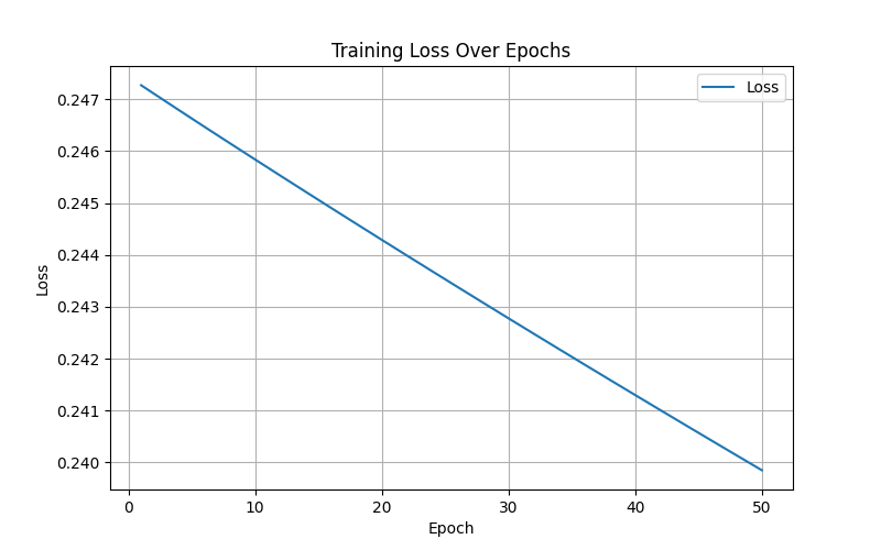
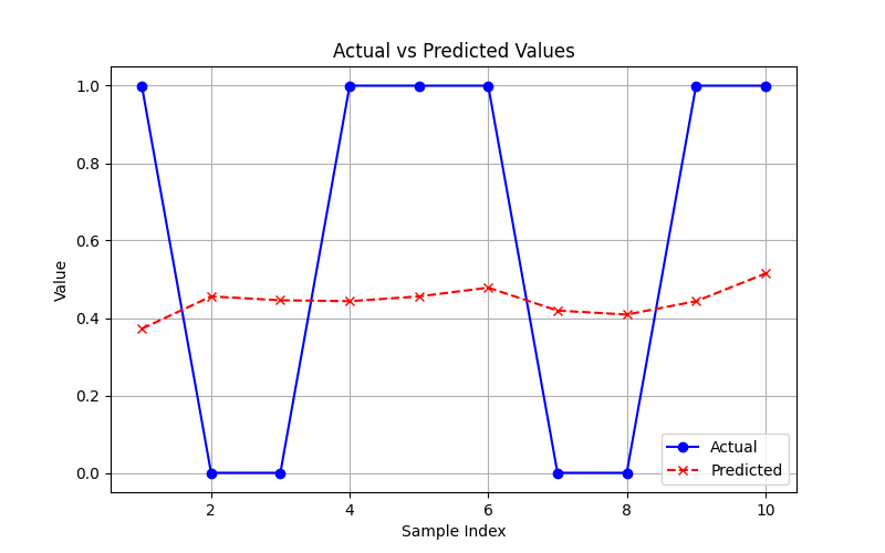
**另外一个实例**
我们假设有一个二维数据集,目标是根据点的位置将它们分类到两个类别中(例如,红色和蓝色点)。
以下实例展示了如何使用神经网络完成简单的二分类任务,为更复杂的任务奠定了基础,通过 PyTorch 的模块化接口,神经网络的构建、训练和可视化都非常直观。
**1、数据准备**
首先,我们生成一些简单的二维数据:
**实例**
```python
import torch
import torch.nn as nn
import torch.optim as optim
import matplotlib.pyplot as plt
# 生成一些随机数据
n_samples = 100
data = torch.randn(n_samples, 2) # 生成 100 个二维数据点
labels = (data[:, 0]**2 + data[:, 1]**2 < 1).float().unsqueeze(1) # 点在圆内为1,圆外为0
# 可视化数据
plt.scatter(data[:, 0], data[:, 1], c=labels.squeeze(), cmap='coolwarm')
plt.title("Generated Data")
plt.xlabel("Feature 1")
plt.ylabel("Feature 2")
plt.show()
```
**数据说明:**
- `data` 是输入的二维点,每个点有两个特征。
- `labels` 是目标分类,点在圆形区域内为 1,否则为 0。
显示如下:
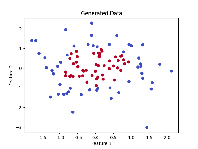
**2、定义神经网络**
用 PyTorch 创建一个简单的前馈神经网络。
前馈神经网络使用了一层隐藏层,通过简单的线性变换和激活函数捕获数据的非线性模式。
**实例**
```python
class SimpleNN(nn.Module):
def __init__(self):
super(SimpleNN, self).__init__()
# 定义神经网络的层
self.fc1 = nn.Linear(2, 4) # 输入层有 2 个特征,隐藏层有 4 个神经元
self.fc2 = nn.Linear(4, 1) # 隐藏层输出到 1 个神经元(用于二分类)
self.sigmoid = nn.Sigmoid() # 二分类激活函数
def forward(self, x):
x = torch.relu(self.fc1(x)) # 使用 ReLU 激活函数
x = self.sigmoid(self.fc2(x)) # 输出层使用 Sigmoid 激活函数
return x
# 实例化模型
model = SimpleNN()
```
**3、定义损失函数和优化器**
**实例**
```python
# 定义二分类的损失函数和优化器
criterion = nn.BCELoss() # 二元交叉熵损失
optimizer = optim.SGD(model.parameters(), lr=0.1) # 使用随机梯度下降优化器
```
**4、训练模型**
用数据训练模型,让它学会分类。
**实例**
```python
# 训练
epochs = 100
for epoch in range(epochs):
# 前向传播
outputs = model(data)
loss = criterion(outputs, labels)
# 反向传播
optimizer.zero_grad()
loss.backward()
optimizer.step()
# 每 10 轮打印一次损失
if (epoch + 1) % 10 == 0:
print(f'Epoch [{epoch + 1}/{epochs}], Loss: {loss.item():.4f}')
```
**5、测试模型并可视化结果**
我们测试模型,并在图像上绘制决策边界。
**实例**
```python
# 可视化决策边界
def plot_decision_boundary(model, data):
x_min, x_max = data[:, 0].min() - 1, data[:, 0].max() + 1
y_min, y_max = data[:, 1].min() - 1, data[:, 1].max() + 1
xx, yy = torch.meshgrid(torch.arange(x_min, x_max, 0.1), torch.arange(y_min, y_max, 0.1), indexing='ij')
grid = torch.cat([xx.reshape(-1, 1), yy.reshape(-1, 1)], dim=1)
predictions = model(grid).detach().numpy().reshape(xx.shape)
plt.contourf(xx, yy, predictions, levels=[0, 0.5, 1], cmap='coolwarm', alpha=0.7)
plt.scatter(data[:, 0], data[:, 1], c=labels.squeeze(), cmap='coolwarm', edgecolors='k')
plt.title("Decision Boundary")
plt.show()
plot_decision_boundary(model, data)
```
**6、完整代码**
完整代码如下:
实例
```python
import torch
import torch.nn as nn
import torch.optim as optim
import matplotlib.pyplot as plt
# 生成一些随机数据
n_samples = 100
data = torch.randn(n_samples, 2) # 生成 100 个二维数据点
labels = (data[:, 0]**2 + data[:, 1]**2 < 1).float().unsqueeze(1) # 点在圆内为1,圆外为0
# 可视化数据
plt.scatter(data[:, 0], data[:, 1], c=labels.squeeze(), cmap='coolwarm')
plt.title("Generated Data")
plt.xlabel("Feature 1")
plt.ylabel("Feature 2")
plt.show()
# 定义前馈神经网络
class SimpleNN(nn.Module):
def __init__(self):
super(SimpleNN, self).__init__()
# 定义神经网络的层
self.fc1 = nn.Linear(2, 4) # 输入层有 2 个特征,隐藏层有 4 个神经元
self.fc2 = nn.Linear(4, 1) # 隐藏层输出到 1 个神经元(用于二分类)
self.sigmoid = nn.Sigmoid() # 二分类激活函数
def forward(self, x):
x = torch.relu(self.fc1(x)) # 使用 ReLU 激活函数
x = self.sigmoid(self.fc2(x)) # 输出层使用 Sigmoid 激活函数
return x
# 实例化模型
model = SimpleNN()
# 定义损失函数和优化器
criterion = nn.BCELoss() # 二元交叉熵损失
optimizer = optim.SGD(model.parameters(), lr=0.1) # 使用随机梯度下降优化器
# 训练
epochs = 2000
for epoch in range(epochs):
# 前向传播
outputs = model(data)
loss = criterion(outputs, labels)
# 反向传播
optimizer.zero_grad()
loss.backward()
optimizer.step()
# 每 10 轮打印一次损失
if (epoch + 1) % 10 == 0:
print(f'Epoch [{epoch + 1}/{epochs}], Loss: {loss.item():.4f}')
# 可视化决策边界
def plot_decision_boundary(model, data):
x_min, x_max = data[:, 0].min() - 1, data[:, 0].max() + 1
y_min, y_max = data[:, 1].min() - 1, data[:, 1].max() + 1
xx, yy = torch.meshgrid(torch.arange(x_min, x_max, 0.1), torch.arange(y_min, y_max, 0.1), indexing='ij')
grid = torch.cat([xx.reshape(-1, 1), yy.reshape(-1, 1)], dim=1)
predictions = model(grid).detach().numpy().reshape(xx.shape)
plt.contourf(xx, yy, predictions, levels=[0, 0.5, 1], cmap='coolwarm', alpha=0.7)
plt.scatter(data[:, 0], data[:, 1], c=labels.squeeze(), cmap='coolwarm', edgecolors='k')
plt.title("Decision Boundary")
plt.show()
plot_decision_boundary(model, data)
```
训练时的损失输出:
```
Epoch [10/2000], Loss: 0.6547
Epoch [20/2000], Loss: 0.6451
Epoch [30/2000], Loss: 0.6363
...
Epoch [1980/2000], Loss: 0.0664
Epoch [1990/2000], Loss: 0.0662
Epoch [2000/2000], Loss: 0.0659
```
图中显示了原始数据点(红色和蓝色),以及模型学习到的分类边界。
# 附录B 大模型自我检测指南
Test Yourself on Build a Large Language Model
关于本书
塞巴斯蒂安·拉施卡(Sebastian Raschka)的畅销书《从零构建大语言模型》(Build a Large Language Model (From Scratch))是学习大语言模型工作原理的最佳途径。全书共七章,另附五个附录,总计350余页,循序渐进地指导你构建一个类似于GPT-2的完整大语言模型。书中使用Python语言和PyTorch深度学习库,采用了一种独特而高效的学习方式——许多人认为,唯有亲手构建模型,才能真正掌握这一领域。
尽管原书已提供了清晰的讲解、图示和代码,但学习如此复杂的主题依然颇具挑战。本《自我检测指南》(Test Yourself guide)旨在让这一过程变得稍微轻松一些。其结构与《从零构建大语言模型》完全对应,聚焦于各章节的核心概念。你可以通过多项选择题、代码与关键概念相关问题,以及需要深入思考的开放式问答题来检验自己的理解。所有题目均附有答案。
无论你当前的知识水平如何,本指南都能以不同方式助你一臂之力:在阅读完某一章后使用它,可巩固所学内容;而在阅读前先浏览它,同样大有裨益——通过预先测试核心概念及其相互关系,你能更轻松地理解章节内容,并为吸收新知识做好准备。
建议在阅读前后都使用本指南,并在日后开始遗忘相关内容时再次回顾。重复学习有助于强化记忆,并将新知识与长期记忆中已有的相关知识有机整合。
## 1 理解大语言模型
第1章对大语言模型(LLM)进行了高层次的概述,探讨了其应用场景、构建阶段以及底层的Transformer架构。本章讨论了预训练(pretraining)和微调(fine-tuning)这两个开发高效LLM的关键步骤,并介绍了Transformer架构及其核心组件,包括编码器(encoder)和解码器(decoder)模块,以及自注意力(self-attention)机制。此外,本章还提出了一个从零开始构建LLM的实施计划,概述了三个主要阶段:数据准备与采样、注意力机制的实现,以及在无标签数据上进行预训练,从而获得一个基础模型,用于后续的微调。
PyTorch 提供了强大的工具来构建和训练神经网络。
神经网络在 PyTorch 中是通过 **torch.nn** 模块来实现的。
**torch.nn** 模块提供了各种网络层(如全连接层、卷积层等)、损失函数和优化器,让神经网络的构建和训练变得更加方便。

在 PyTorch 中,构建神经网络通常需要继承 nn.Module 类。
nn.Module 是所有神经网络模块的基类,你需要定义以下两个部分:
- **`__init__()`**:定义网络层。
- **`forward()`**:定义数据的前向传播过程。
简单的全连接神经网络(Fully Connected Network):
**实例**
```python
import torch
import torch.nn as nn
# 定义一个简单的神经网络模型
class SimpleNN(nn.Module):
def init(self):
super(SimpleNN, self).init()
# 定义一个输入层到隐藏层的全连接层
self.fc1 = nn.Linear(2, 2) # 输入 2 个特征,输出 2 个特征
# 定义一个隐藏层到输出层的全连接层
self.fc2 = nn.Linear(2, 1) # 输入 2 个特征,输出 1 个预测值
def forward(self, x):
# 前向传播过程
x = torch.relu(self.fc1(x)) # 使用 ReLU 激活函数
x = self.fc2(x) # 输出层
return x
# 创建模型实例
model = SimpleNN()
# 打印模型
print(model)
```
输出结果如下:
```
SimpleNN(
(fc1): Linear(in_features=2, out_features=2, bias=True)
(fc2): Linear(in_features=2, out_features=1, bias=True)
)
```
PyTorch 提供了许多常见的神经网络层,以下是几个常见的:
- **`nn.Linear(in_features, out_features)`**:全连接层,输入 `in_features` 个特征,输出 `out_features` 个特征。
- **`nn.Conv2d(in_channels, out_channels, kernel_size)`**:2D 卷积层,用于图像处理。
- **`nn.MaxPool2d(kernel_size)`**:2D 最大池化层,用于降维。
- **`nn.ReLU()`**:ReLU 激活函数,常用于隐藏层。
- **`nn.Softmax(dim)`**:Softmax 激活函数,通常用于输出层,适用于多类分类问题。
**激活函数(Activation Function)**
激活函数决定了神经元是否应该被激活。它们是非线性函数,使得神经网络能够学习和执行更复杂的任务。常见的激活函数包括:
- Sigmoid:用于二分类问题,输出值在 0 和 1 之间。
- Tanh:输出值在 -1 和 1 之间,常用于输出层之前。
- ReLU(Rectified Linear Unit):目前最流行的激活函数之一,定义为 `f(x) = max(0, x)`,有助于解决梯度消失问题。
- Softmax:常用于多分类问题的输出层,将输出转换为概率分布。
**实例**
```python
import torch.nn.functional as F
# ReLU 激活
output = F.relu(input_tensor)
# Sigmoid 激活
output = torch.sigmoid(input_tensor)
# Tanh 激活
output = torch.tanh(input_tensor)
```
**损失函数(Loss Function)**
损失函数用于衡量模型的预测值与真实值之间的差异。
常见的损失函数包括:
- **均方误差(MSELoss)**:回归问题常用,计算输出与目标值的平方差。
- **交叉熵损失(CrossEntropyLoss)**:分类问题常用,计算输出和真实标签之间的交叉熵。
- **BCEWithLogitsLoss**:二分类问题,结合了 Sigmoid 激活和二元交叉熵损失。
**实例**
```python
# 均方误差损失
criterion = nn.MSELoss()
# 交叉熵损失
criterion = nn.CrossEntropyLoss()
# 二分类交叉熵损失
criterion = nn.BCEWithLogitsLoss()
```
**优化器(Optimizer)**
优化器负责在训练过程中更新网络的权重和偏置。
常见的优化器包括:
- SGD(随机梯度下降)
- Adam(自适应矩估计)
- RMSprop(均方根传播)
**实例**
```python
import torch.optim as optim
# 使用 SGD 优化器
optimizer = optim.SGD(model.parameters(), lr=0.01)
# 使用 Adam 优化器
optimizer = optim.Adam(model.parameters(), lr=0.001)
```
**训练过程(Training Process)**
训练神经网络涉及以下步骤:
1. **准备数据**:通过 `DataLoader` 加载数据。
2. **定义损失函数和优化器**。
3. **前向传播**:计算模型的输出。
4. **计算损失**:与目标进行比较,得到损失值。
5. **反向传播**:通过 `loss.backward()` 计算梯度。
6. **更新参数**:通过 `optimizer.step()` 更新模型的参数。
7. **重复上述步骤**,直到达到预定的训练轮数。
**实例**
```python
\# 假设已经定义好了模型、损失函数和优化器
\# 训练数据示例
X = torch.randn(10, 2) # 10 个样本,每个样本有 2 个特征
Y = torch.randn(10, 1) # 10 个目标标签
\# 训练过程
for epoch in range(100): # 训练 100 轮
model.train() # 设置模型为训练模式
optimizer.zero_grad() # 清除梯度
output = model(X) # 前向传播
loss = criterion(output, Y) # 计算损失
loss.backward() # 反向传播
optimizer.step() # 更新权重
if (epoch + 1) % 10 == 0: # 每 10 轮输出一次损失
print(f'Epoch [{epoch + 1}/100], Loss: {loss.item():.4f}')
```
**测试与评估**
训练完成后,需要对模型进行测试和评估。
常见的步骤包括:
- **计算测试集的损失**:测试模型在未见过的数据上的表现。
- **计算准确率(Accuracy)**:对于分类问题,计算正确预测的比例。
**实例**
```python
# 假设你有测试集 X_test 和 Y_test
model.eval() # 设置模型为评估模式
with torch.no_grad(): # 在评估过程中禁用梯度计算
output = model(X_test)
loss = criterion(output, Y_test)
print(f'Test Loss: {loss.item():.4f}')
```
**神经网络类型**
1. **前馈神经网络(Feedforward Neural Networks)**:数据单向流动,从输入层到输出层,无反馈连接。
2. **卷积神经网络(Convolutional Neural Networks, CNNs)**:适用于图像处理,使用卷积层提取空间特征。
3. **循环神经网络(Recurrent Neural Networks, RNNs)**:适用于序列数据,如时间序列分析和自然语言处理,允许信息反馈循环。
4. **长短期记忆网络(Long Short-Term Memory, LSTM)**:一种特殊的RNN,能够学习长期依赖关系。
## A.6 PyTorch 第一个神经网络
本章节我们将介绍如何用 PyTorch 实现一个简单的前馈神经网络,完成一个二分类任务。
以下实例展示了如何使用 PyTorch 实现一个简单的神经网络进行二分类任务训练。
网络结构包括输入层、隐藏层和输出层,使用了 ReLU 激活函数和 Sigmoid 激活函数。
采用了均方误差损失函数和随机梯度下降优化器。
训练过程是通过前向传播、计算损失、反向传播和参数更新来逐步调整模型参数。
**实例**
```python
# 导入PyTorch库
import torch
import torch.nn as nn
# 定义输入层大小、隐藏层大小、输出层大小和批量大小
n_in, n_h, n_out, batch_size = 10, 5, 1, 10
# 创建虚拟输入数据和目标数据
x = torch.randn(batch_size, n_in) # 随机生成输入数据
y = torch.tensor([[1.0], [0.0], [0.0],
[1.0], [1.0], [1.0], [0.0], [0.0], [1.0], [1.0]]) # 目标输出数据
# 创建顺序模型,包含线性层、ReLU激活函数和Sigmoid激活函数
model = nn.Sequential(
nn.Linear(n_in, n_h), # 输入层到隐藏层的线性变换
nn.ReLU(), # 隐藏层的ReLU激活函数
nn.Linear(n_h, n_out), # 隐藏层到输出层的线性变换
nn.Sigmoid() # 输出层的Sigmoid激活函数
)
# 定义均方误差损失函数和随机梯度下降优化器
criterion = torch.nn.MSELoss()
optimizer = torch.optim.SGD(model.parameters(), lr=0.01) # 学习率为0.01
# 执行梯度下降算法进行模型训练
for epoch in range(50): # 迭代50次
y_pred = model(x) # 前向传播,计算预测值
loss = criterion(y_pred, y) # 计算损失
print('epoch: ', epoch, 'loss: ', loss.item()) # 打印损失值
optimizer.zero_grad() # 清零梯度
loss.backward() # 反向传播,计算梯度
optimizer.step() # 更新模型参数
```
输出结果类似如下:
```
epoch: 0 loss: 0.2302265167236328
epoch: 1 loss: 0.23012931644916534
epoch: 2 loss: 0.23003216087818146
epoch: 3 loss: 0.22993502020835876
epoch: 4 loss: 0.22983793914318085
...
```
定义网络参数:
```
n_in, n_h, n_out, batch_size = 10, 5, 1, 10
```
- `n_in`:输入层大小为 10,即每个数据点有 10 个特征。
- `n_h`:隐藏层大小为 5,即隐藏层包含 5 个神经元。
- `n_out`:输出层大小为 1,即输出一个标量,表示二分类结果(0 或 1)。
- `batch_size`:每个批次包含 10 个样本。
生成输入数据和目标数据:
```python
x = torch.randn(batch_size, n_in) # 随机生成输入数据
y = torch.tensor([[1.0], [0.0], [0.0],
[1.0], [1.0], [1.0], [0.0], [0.0], [1.0], [1.0]]) # 目标输出数据
```
- `x`:随机生成一个形状为 `(10, 10)` 的输入数据矩阵,表示 10 个样本,每个样本有 10 个特征。
- `y`:目标输出数据(标签),表示每个输入样本的类别标签(0 或 1),是一个 10×1 的张量。
定义神经网络模型:
```python
model = nn.Sequential(
nn.Linear(n_in, n_h), # 输入层到隐藏层的线性变换
nn.ReLU(), # 隐藏层的ReLU激活函数
nn.Linear(n_h, n_out), # 隐藏层到输出层的线性变换
nn.Sigmoid() # 输出层的Sigmoid激活函数
)
```
`nn.Sequential` 用于按顺序定义网络层。
- `nn.Linear(n_in, n_h)`:定义输入层到隐藏层的线性变换,输入特征是 10 个,隐藏层有 5 个神经元。
- `nn.ReLU()`:在隐藏层后添加 ReLU 激活函数,增加非线性。
- `nn.Linear(n_h, n_out)`:定义隐藏层到输出层的线性变换,输出为 1 个神经元。
- `nn.Sigmoid()`:输出层使用 Sigmoid 激活函数,将结果映射到 0 到 1 之间,用于二分类任务。
定义损失函数和优化器:
```python
criterion = torch.nn.MSELoss() # 使用均方误差损失函数
optimizer = torch.optim.SGD(model.parameters(), lr=0.01) # 使用随机梯度下降优化器,学习率为 0.01
```
训练循环:
```python
for epoch in range(50): # 训练50轮
y_pred = model(x) # 前向传播,计算预测值
loss = criterion(y_pred, y) # 计算损失
print('epoch: ', epoch, 'loss: ', loss.item()) # 打印损失值
optimizer.zero_grad() # 清零梯度
loss.backward() # 反向传播,计算梯度
optimizer.step() # 更新模型参数
```
- `for epoch in range(50)`:进行 50 次训练迭代。
- `y_pred = model(x)`:进行前向传播,使用当前模型参数计算输入数据 `x` 的预测值。
- `loss = criterion(y_pred, y)`:计算预测值和目标值 `y` 之间的损失。
- `optimizer.zero_grad()`:清除上一轮训练时的梯度值。
- `loss.backward()`:反向传播,计算损失函数相对于模型参数的梯度。
- `optimizer.step()`:根据计算出的梯度更新模型参数。
可视化代码:
**实例**
```python
import torch
import torch.nn as nn
import matplotlib.pyplot as plt
# 定义输入层大小、隐藏层大小、输出层大小和批量大小
n_in, n_h, n_out, batch_size = 10, 5, 1, 10
# 创建虚拟输入数据和目标数据
x = torch.randn(batch_size, n_in) # 随机生成输入数据
y = torch.tensor([[1.0], [0.0], [0.0],
[1.0], [1.0], [1.0], [0.0], [0.0], [1.0], [1.0]]) # 目标输出数据
# 创建顺序模型,包含线性层、ReLU激活函数和Sigmoid激活函数
model = nn.Sequential(
nn.Linear(n_in, n_h), # 输入层到隐藏层的线性变换
nn.ReLU(), # 隐藏层的ReLU激活函数
nn.Linear(n_h, n_out), # 隐藏层到输出层的线性变换
nn.Sigmoid() # 输出层的Sigmoid激活函数
)
# 定义均方误差损失函数和随机梯度下降优化器
criterion = torch.nn.MSELoss()
optimizer = torch.optim.SGD(model.parameters(), lr=0.01) # 学习率为0.01
# 用于存储每轮的损失值
losses = []
# 执行梯度下降算法进行模型训练
for epoch in range(50): # 迭代50次
y_pred = model(x) # 前向传播,计算预测值
loss = criterion(y_pred, y) # 计算损失
losses.append(loss.item()) # 记录损失值
print(f'Epoch [{epoch+1}/50], Loss: {loss.item():.4f}') # 打印损失值
optimizer.zero_grad() # 清零梯度
loss.backward() # 反向传播,计算梯度
optimizer.step() # 更新模型参数
# 可视化损失变化曲线
plt.figure(figsize=(8, 5))
plt.plot(range(1, 51), losses, label='Loss')
plt.xlabel('Epoch')
plt.ylabel('Loss')
plt.title('Training Loss Over Epochs')
plt.legend()
plt.grid()
plt.show()
# 可视化预测结果与实际目标值对比
y_pred_final = model(x).detach().numpy() # 最终预测值
y_actual = y.numpy() # 实际值
plt.figure(figsize=(8, 5))
plt.plot(range(1, batch_size + 1), y_actual, 'o-', label='Actual', color='blue')
plt.plot(range(1, batch_size + 1), y_pred_final, 'x--', label='Predicted', color='red')
plt.xlabel('Sample Index')
plt.ylabel('Value')
plt.title('Actual vs Predicted Values')
plt.legend()
plt.grid()
plt.show()
```
显示如下所示:


**另外一个实例**
我们假设有一个二维数据集,目标是根据点的位置将它们分类到两个类别中(例如,红色和蓝色点)。
以下实例展示了如何使用神经网络完成简单的二分类任务,为更复杂的任务奠定了基础,通过 PyTorch 的模块化接口,神经网络的构建、训练和可视化都非常直观。
**1、数据准备**
首先,我们生成一些简单的二维数据:
**实例**
```python
import torch
import torch.nn as nn
import torch.optim as optim
import matplotlib.pyplot as plt
# 生成一些随机数据
n_samples = 100
data = torch.randn(n_samples, 2) # 生成 100 个二维数据点
labels = (data[:, 0]**2 + data[:, 1]**2 < 1).float().unsqueeze(1) # 点在圆内为1,圆外为0
# 可视化数据
plt.scatter(data[:, 0], data[:, 1], c=labels.squeeze(), cmap='coolwarm')
plt.title("Generated Data")
plt.xlabel("Feature 1")
plt.ylabel("Feature 2")
plt.show()
```
**数据说明:**
- `data` 是输入的二维点,每个点有两个特征。
- `labels` 是目标分类,点在圆形区域内为 1,否则为 0。
显示如下:

**2、定义神经网络**
用 PyTorch 创建一个简单的前馈神经网络。
前馈神经网络使用了一层隐藏层,通过简单的线性变换和激活函数捕获数据的非线性模式。
**实例**
```python
class SimpleNN(nn.Module):
def __init__(self):
super(SimpleNN, self).__init__()
# 定义神经网络的层
self.fc1 = nn.Linear(2, 4) # 输入层有 2 个特征,隐藏层有 4 个神经元
self.fc2 = nn.Linear(4, 1) # 隐藏层输出到 1 个神经元(用于二分类)
self.sigmoid = nn.Sigmoid() # 二分类激活函数
def forward(self, x):
x = torch.relu(self.fc1(x)) # 使用 ReLU 激活函数
x = self.sigmoid(self.fc2(x)) # 输出层使用 Sigmoid 激活函数
return x
# 实例化模型
model = SimpleNN()
```
**3、定义损失函数和优化器**
**实例**
```python
# 定义二分类的损失函数和优化器
criterion = nn.BCELoss() # 二元交叉熵损失
optimizer = optim.SGD(model.parameters(), lr=0.1) # 使用随机梯度下降优化器
```
**4、训练模型**
用数据训练模型,让它学会分类。
**实例**
```python
# 训练
epochs = 100
for epoch in range(epochs):
# 前向传播
outputs = model(data)
loss = criterion(outputs, labels)
# 反向传播
optimizer.zero_grad()
loss.backward()
optimizer.step()
# 每 10 轮打印一次损失
if (epoch + 1) % 10 == 0:
print(f'Epoch [{epoch + 1}/{epochs}], Loss: {loss.item():.4f}')
```
**5、测试模型并可视化结果**
我们测试模型,并在图像上绘制决策边界。
**实例**
```python
# 可视化决策边界
def plot_decision_boundary(model, data):
x_min, x_max = data[:, 0].min() - 1, data[:, 0].max() + 1
y_min, y_max = data[:, 1].min() - 1, data[:, 1].max() + 1
xx, yy = torch.meshgrid(torch.arange(x_min, x_max, 0.1), torch.arange(y_min, y_max, 0.1), indexing='ij')
grid = torch.cat([xx.reshape(-1, 1), yy.reshape(-1, 1)], dim=1)
predictions = model(grid).detach().numpy().reshape(xx.shape)
plt.contourf(xx, yy, predictions, levels=[0, 0.5, 1], cmap='coolwarm', alpha=0.7)
plt.scatter(data[:, 0], data[:, 1], c=labels.squeeze(), cmap='coolwarm', edgecolors='k')
plt.title("Decision Boundary")
plt.show()
plot_decision_boundary(model, data)
```
**6、完整代码**
完整代码如下:
实例
```python
import torch
import torch.nn as nn
import torch.optim as optim
import matplotlib.pyplot as plt
# 生成一些随机数据
n_samples = 100
data = torch.randn(n_samples, 2) # 生成 100 个二维数据点
labels = (data[:, 0]**2 + data[:, 1]**2 < 1).float().unsqueeze(1) # 点在圆内为1,圆外为0
# 可视化数据
plt.scatter(data[:, 0], data[:, 1], c=labels.squeeze(), cmap='coolwarm')
plt.title("Generated Data")
plt.xlabel("Feature 1")
plt.ylabel("Feature 2")
plt.show()
# 定义前馈神经网络
class SimpleNN(nn.Module):
def __init__(self):
super(SimpleNN, self).__init__()
# 定义神经网络的层
self.fc1 = nn.Linear(2, 4) # 输入层有 2 个特征,隐藏层有 4 个神经元
self.fc2 = nn.Linear(4, 1) # 隐藏层输出到 1 个神经元(用于二分类)
self.sigmoid = nn.Sigmoid() # 二分类激活函数
def forward(self, x):
x = torch.relu(self.fc1(x)) # 使用 ReLU 激活函数
x = self.sigmoid(self.fc2(x)) # 输出层使用 Sigmoid 激活函数
return x
# 实例化模型
model = SimpleNN()
# 定义损失函数和优化器
criterion = nn.BCELoss() # 二元交叉熵损失
optimizer = optim.SGD(model.parameters(), lr=0.1) # 使用随机梯度下降优化器
# 训练
epochs = 2000
for epoch in range(epochs):
# 前向传播
outputs = model(data)
loss = criterion(outputs, labels)
# 反向传播
optimizer.zero_grad()
loss.backward()
optimizer.step()
# 每 10 轮打印一次损失
if (epoch + 1) % 10 == 0:
print(f'Epoch [{epoch + 1}/{epochs}], Loss: {loss.item():.4f}')
# 可视化决策边界
def plot_decision_boundary(model, data):
x_min, x_max = data[:, 0].min() - 1, data[:, 0].max() + 1
y_min, y_max = data[:, 1].min() - 1, data[:, 1].max() + 1
xx, yy = torch.meshgrid(torch.arange(x_min, x_max, 0.1), torch.arange(y_min, y_max, 0.1), indexing='ij')
grid = torch.cat([xx.reshape(-1, 1), yy.reshape(-1, 1)], dim=1)
predictions = model(grid).detach().numpy().reshape(xx.shape)
plt.contourf(xx, yy, predictions, levels=[0, 0.5, 1], cmap='coolwarm', alpha=0.7)
plt.scatter(data[:, 0], data[:, 1], c=labels.squeeze(), cmap='coolwarm', edgecolors='k')
plt.title("Decision Boundary")
plt.show()
plot_decision_boundary(model, data)
```
训练时的损失输出:
```
Epoch [10/2000], Loss: 0.6547
Epoch [20/2000], Loss: 0.6451
Epoch [30/2000], Loss: 0.6363
...
Epoch [1980/2000], Loss: 0.0664
Epoch [1990/2000], Loss: 0.0662
Epoch [2000/2000], Loss: 0.0659
```
图中显示了原始数据点(红色和蓝色),以及模型学习到的分类边界。

# 附录B 大模型自我检测指南
Test Yourself on Build a Large Language Model
关于本书
塞巴斯蒂安·拉施卡(Sebastian Raschka)的畅销书《从零构建大语言模型》(Build a Large Language Model (From Scratch))是学习大语言模型工作原理的最佳途径。全书共七章,另附五个附录,总计350余页,循序渐进地指导你构建一个类似于GPT-2的完整大语言模型。书中使用Python语言和PyTorch深度学习库,采用了一种独特而高效的学习方式——许多人认为,唯有亲手构建模型,才能真正掌握这一领域。
尽管原书已提供了清晰的讲解、图示和代码,但学习如此复杂的主题依然颇具挑战。本《自我检测指南》(Test Yourself guide)旨在让这一过程变得稍微轻松一些。其结构与《从零构建大语言模型》完全对应,聚焦于各章节的核心概念。你可以通过多项选择题、代码与关键概念相关问题,以及需要深入思考的开放式问答题来检验自己的理解。所有题目均附有答案。
无论你当前的知识水平如何,本指南都能以不同方式助你一臂之力:在阅读完某一章后使用它,可巩固所学内容;而在阅读前先浏览它,同样大有裨益——通过预先测试核心概念及其相互关系,你能更轻松地理解章节内容,并为吸收新知识做好准备。
建议在阅读前后都使用本指南,并在日后开始遗忘相关内容时再次回顾。重复学习有助于强化记忆,并将新知识与长期记忆中已有的相关知识有机整合。
## 1 理解大语言模型
第1章对大语言模型(LLM)进行了高层次的概述,探讨了其应用场景、构建阶段以及底层的Transformer架构。本章讨论了预训练(pretraining)和微调(fine-tuning)这两个开发高效LLM的关键步骤,并介绍了Transformer架构及其核心组件,包括编码器(encoder)和解码器(decoder)模块,以及自注意力(self-attention)机制。此外,本章还提出了一个从零开始构建LLM的实施计划,概述了三个主要阶段:数据准备与采样、注意力机制的实现,以及在无标签数据上进行预训练,从而获得一个基础模型,用于后续的微调。
 ### **核心概念快速问答**
1. 在大语言模型的背景下,深度学习与传统机器学习的主要区别是什么?
A. 深度学习更适合处理结构化数据,而传统机器学习更适合非结构化数据。
**B. 深度学习无需手动特征提取,而传统机器学习需要。**
C. 深度学习在所有任务上都比传统机器学习更准确。
D. 深度学习比传统机器学习计算效率更高。
2. 大语言模型(LLM)的主要功能是什么?
A. 分析和解读图像。
B. 预测未来事件。
**C. 理解、生成并回应类人文本。**
D. 控制和操作机器人。
3. 与通用大语言模型相比,定制构建的大语言模型(custom-built LLMs)的主要优势是什么?
**A. 它们在特定任务或领域中可以超越通用大语言模型。**
B. 它们更具通用性,可用于更广泛的任务。
C. 它们在处理大型数据集时效率更高。
D. 它们的训练成本更低。
4. Transformer架构在大语言模型中的重要意义是什么?
A. 它为大型数据集提供了更快的处理速度。
**B. 它使模型在进行预测时能够有选择性地关注输入文本的不同部分。**
C. 它使模型能够从未标注的数据中学习。
D. 它使模型无需专门训练即可实现语言翻译。
5. 对大语言模型进行预训练(pretraining)的主要目的是什么?
A. 为特定任务微调模型。
B. 评估模型在各种任务上的表现。
C. 创建一个能够翻译语言的模型。
**D. 通过在大规模、多样化的数据集上训练,使模型获得对语言的广泛理解。**
**按章节小节划分的问题**
接下来,将更详细地逐节回顾本章内容。
### 1.1 什么是大语言模型?
1. 什么是大语言模型(LLM)?它是如何工作的?
An LLM is a deep neural network trained on massive amounts of text data to understand, generate, and respond to human-like text. It uses a transformer architecture to pay attention to different parts of the input, making it adept at handling language nuances. LLMs are trained on the task of predicting the next word in a sequence, which allows them to
learn context, structure, and relationships within text.
2. “大语言模型”中的“大”有何重要意义?
The 'large' refers to both the model's size in terms of parameters (adjustable weights) and the immense dataset it's trained on. LLMs often have tens or hundreds of billions of parameters, which are optimized during training to predict the next word in a sequence.
3. How do LLMs relate to generative AI?
LLMs are often considered a form of generative AI because they can generate text. Generative AI is a broader term encompassing AI systems that create new content, such as text, images, or music.
4. Label this diagram
5. What is the difference between traditional machine learning and deep learning in terms of feature extraction?
AI is the broader field of creating machines that can perform tasks requiring human-like intelligence. Machine learning is a subset of AI that focuses on algorithms that learn from data. Deep learning is a subset of machine learning that uses deep neural networks with multiple layers to model complex patterns in data
6. 将术语与其右侧的描述进行匹配:
| Large Language Model (LLM) | | A subset of machine learning that uses deep neural networks to model complex patterns and abstractions in data. |
| -------------------------- | ---- | ------------------------------------------------------------ |
| Transformer | | A type of artificial intelligence that can create new content, such as text, images, or audio. |
| Generative AI | | An architecture used in LLMs that allows them to pay selective attention to different parts of the input when making predictions, making them adept at handling the nuances of human language. |
| Deep Learning | | A type of artificial intelligence that uses deep learning to understand, generate, and respond to human-like text. |
Fill the table with the column mappings:
| Left Hand Column | 1 | 2 | 3 | 4 |
| ----------------- | ---- | ---- | ---- | ---- |
| Right Hand Column | 4 | 3 | 2 | 1 |
### 1.2 大语言模型的应用
1. What are some of the key applications of LLMs in various domains?
LLMs are used in machine translation, text generation, sentiment analysis, text summarization, content creation, powering chatbots and virtual assistants, and knowledge retrieval from specialized areas like medicine and law.
2. How do LLMs contribute to the development of chatbots and virtual assistants?
LLMs enable chatbots and virtual assistants like ChatGPT and Gemini to understand and respond to user queries in a natural language, enhancing their ability to provide information and complete tasks.
3. Explain the role of LLMs in knowledge retrieval from specialized fields.
LLMs can analyze vast amounts of text in fields like medicine or law, summarizing lengthy passages, answering technical questions, and facilitating efficient knowledge retrieval.
4. What is the potential impact of LLMs on our relationship with technology?
LLMs have the potential to make technology more conversational, intuitive, and accessible by automating text-based tasks and enabling natural language interactions with AI systems.
5. 将术语与其右侧的描述进行匹配:
| Natural Language Processing | | a field of computer science that focuses on enabling computers to understand and process human language. |
| --------------------------- | ---- | ------------------------------------------------------------ |
| Machine Translation | | computer programs designed to simulate conversation with human users. |
| Chatbots | | the process of extracting relevant information from large amounts of data. |
| Knowledge Retrieval | | the automatic translation of text from one language to another. |
Fill the table with the column mappings:
| Left Hand Column | 1 | 2 | 3 | 4 |
| ----------------- | ---- | ---- | ---- | ---- |
| Right Hand Column | 1 | 4 | 2 | 3 |
### 1.3 构建和使用大语言模型的各个阶段
1. What are the main advantages of building custom LLMs compared to using general-purpose LLMs like ChatGPT?
Custom LLMs offer advantages like improved performance for specific tasks or domains, enhanced data privacy by avoiding reliance on thirdparty providers, and the ability to deploy models locally on devices for reduced latency and costs.
2. Describe the two-stage training process involved in creating an LLM.
The process begins with pretraining, where the model learns a broad understanding of language from a large, diverse dataset. This pretrained model is then fine-tuned on a smaller, more specific dataset to adapt it to particular tasks or domains.
3. What is the purpose of pretraining an LLM, and what type of data is used in this stage?
Pretraining aims to develop a foundational model with a general understanding of language. It uses large amounts of unlabeled text data, often referred to as 'raw' text, to train the model to predict the next word in a sequence.
4. Explain the concept of self-supervised learning in the context of pretraining LLMs.
Self-supervised learning allows LLMs to generate their own labels from the input data during pretraining. This eliminates the need for manually labeled data, which is a common requirement in traditional supervised learning.
5. What are the two main categories of fine-tuning LLMs, and how do they differ in terms of the labeled data used?
Instruction fine-tuning uses labeled data consisting of instruction-answer pairs, while classification fine-tuning uses labeled data with texts and associated class labels.
6. 将术语与其右侧的描述进行匹配:
| Pretraining | | A type of fine-tuning where the labeled dataset consists of instruction and answer pairs, such as a query to translate a text accompanied by the correctly translated text. |
| -------------------------- | ---- | ------------------------------------------------------------ |
| Fine-tuning | | A type of fine-tuning where the labeled dataset consists of texts and associated class labels, for example, emails associated with "spam" and "not spam" labels. |
| Instruction Fine-tuning | | The process of further training a pretrained LLM on a narrower dataset that is more specific to particular tasks or domains. |
| Classification Fine-tuning | | The initial phase of training an LLM on a large, diverse dataset to develop a broad understanding of language. |
Fill the table with the column mappings:
| Left Hand Column | 1 | 2 | 3 | 4 |
| ----------------- | ---- | ---- | ---- | ---- |
| Right Hand Column | 4 | 3 | 1 | 2 |
### 1.4 Transformer架构介绍
1. What is the transformer architecture and what is its significance in the development of LLMs?
The transformer architecture is a deep neural network architecture that revolutionized natural language processing. It's the foundation for most modern LLMs, enabling them to process and understand language effectively.
2. Which label in the diagram does the output of the Embeddings stage go to?
The output of the Embeddings stage goes to the Decoder, label 2.
大部分的现代大语言模型基于Transformer架构,这是一种深度神经网络架构,该架构是在谷歌于2017年发表的论文“Attention Is All You Need”中首次提出的。为了理解大语言模型,我们需要简单回顾一下最初的Transformer。Transformer最初是为机器翻译任务(比如将英文翻译成德语和法语)开发的。Transformer架构的一个简化版本如图1-4所示。
### **核心概念快速问答**
1. 在大语言模型的背景下,深度学习与传统机器学习的主要区别是什么?
A. 深度学习更适合处理结构化数据,而传统机器学习更适合非结构化数据。
**B. 深度学习无需手动特征提取,而传统机器学习需要。**
C. 深度学习在所有任务上都比传统机器学习更准确。
D. 深度学习比传统机器学习计算效率更高。
2. 大语言模型(LLM)的主要功能是什么?
A. 分析和解读图像。
B. 预测未来事件。
**C. 理解、生成并回应类人文本。**
D. 控制和操作机器人。
3. 与通用大语言模型相比,定制构建的大语言模型(custom-built LLMs)的主要优势是什么?
**A. 它们在特定任务或领域中可以超越通用大语言模型。**
B. 它们更具通用性,可用于更广泛的任务。
C. 它们在处理大型数据集时效率更高。
D. 它们的训练成本更低。
4. Transformer架构在大语言模型中的重要意义是什么?
A. 它为大型数据集提供了更快的处理速度。
**B. 它使模型在进行预测时能够有选择性地关注输入文本的不同部分。**
C. 它使模型能够从未标注的数据中学习。
D. 它使模型无需专门训练即可实现语言翻译。
5. 对大语言模型进行预训练(pretraining)的主要目的是什么?
A. 为特定任务微调模型。
B. 评估模型在各种任务上的表现。
C. 创建一个能够翻译语言的模型。
**D. 通过在大规模、多样化的数据集上训练,使模型获得对语言的广泛理解。**
**按章节小节划分的问题**
接下来,将更详细地逐节回顾本章内容。
### 1.1 什么是大语言模型?
1. 什么是大语言模型(LLM)?它是如何工作的?
An LLM is a deep neural network trained on massive amounts of text data to understand, generate, and respond to human-like text. It uses a transformer architecture to pay attention to different parts of the input, making it adept at handling language nuances. LLMs are trained on the task of predicting the next word in a sequence, which allows them to
learn context, structure, and relationships within text.
2. “大语言模型”中的“大”有何重要意义?
The 'large' refers to both the model's size in terms of parameters (adjustable weights) and the immense dataset it's trained on. LLMs often have tens or hundreds of billions of parameters, which are optimized during training to predict the next word in a sequence.
3. How do LLMs relate to generative AI?
LLMs are often considered a form of generative AI because they can generate text. Generative AI is a broader term encompassing AI systems that create new content, such as text, images, or music.
4. Label this diagram
5. What is the difference between traditional machine learning and deep learning in terms of feature extraction?
AI is the broader field of creating machines that can perform tasks requiring human-like intelligence. Machine learning is a subset of AI that focuses on algorithms that learn from data. Deep learning is a subset of machine learning that uses deep neural networks with multiple layers to model complex patterns in data
6. 将术语与其右侧的描述进行匹配:
| Large Language Model (LLM) | | A subset of machine learning that uses deep neural networks to model complex patterns and abstractions in data. |
| -------------------------- | ---- | ------------------------------------------------------------ |
| Transformer | | A type of artificial intelligence that can create new content, such as text, images, or audio. |
| Generative AI | | An architecture used in LLMs that allows them to pay selective attention to different parts of the input when making predictions, making them adept at handling the nuances of human language. |
| Deep Learning | | A type of artificial intelligence that uses deep learning to understand, generate, and respond to human-like text. |
Fill the table with the column mappings:
| Left Hand Column | 1 | 2 | 3 | 4 |
| ----------------- | ---- | ---- | ---- | ---- |
| Right Hand Column | 4 | 3 | 2 | 1 |
### 1.2 大语言模型的应用
1. What are some of the key applications of LLMs in various domains?
LLMs are used in machine translation, text generation, sentiment analysis, text summarization, content creation, powering chatbots and virtual assistants, and knowledge retrieval from specialized areas like medicine and law.
2. How do LLMs contribute to the development of chatbots and virtual assistants?
LLMs enable chatbots and virtual assistants like ChatGPT and Gemini to understand and respond to user queries in a natural language, enhancing their ability to provide information and complete tasks.
3. Explain the role of LLMs in knowledge retrieval from specialized fields.
LLMs can analyze vast amounts of text in fields like medicine or law, summarizing lengthy passages, answering technical questions, and facilitating efficient knowledge retrieval.
4. What is the potential impact of LLMs on our relationship with technology?
LLMs have the potential to make technology more conversational, intuitive, and accessible by automating text-based tasks and enabling natural language interactions with AI systems.
5. 将术语与其右侧的描述进行匹配:
| Natural Language Processing | | a field of computer science that focuses on enabling computers to understand and process human language. |
| --------------------------- | ---- | ------------------------------------------------------------ |
| Machine Translation | | computer programs designed to simulate conversation with human users. |
| Chatbots | | the process of extracting relevant information from large amounts of data. |
| Knowledge Retrieval | | the automatic translation of text from one language to another. |
Fill the table with the column mappings:
| Left Hand Column | 1 | 2 | 3 | 4 |
| ----------------- | ---- | ---- | ---- | ---- |
| Right Hand Column | 1 | 4 | 2 | 3 |
### 1.3 构建和使用大语言模型的各个阶段
1. What are the main advantages of building custom LLMs compared to using general-purpose LLMs like ChatGPT?
Custom LLMs offer advantages like improved performance for specific tasks or domains, enhanced data privacy by avoiding reliance on thirdparty providers, and the ability to deploy models locally on devices for reduced latency and costs.
2. Describe the two-stage training process involved in creating an LLM.
The process begins with pretraining, where the model learns a broad understanding of language from a large, diverse dataset. This pretrained model is then fine-tuned on a smaller, more specific dataset to adapt it to particular tasks or domains.
3. What is the purpose of pretraining an LLM, and what type of data is used in this stage?
Pretraining aims to develop a foundational model with a general understanding of language. It uses large amounts of unlabeled text data, often referred to as 'raw' text, to train the model to predict the next word in a sequence.
4. Explain the concept of self-supervised learning in the context of pretraining LLMs.
Self-supervised learning allows LLMs to generate their own labels from the input data during pretraining. This eliminates the need for manually labeled data, which is a common requirement in traditional supervised learning.
5. What are the two main categories of fine-tuning LLMs, and how do they differ in terms of the labeled data used?
Instruction fine-tuning uses labeled data consisting of instruction-answer pairs, while classification fine-tuning uses labeled data with texts and associated class labels.
6. 将术语与其右侧的描述进行匹配:
| Pretraining | | A type of fine-tuning where the labeled dataset consists of instruction and answer pairs, such as a query to translate a text accompanied by the correctly translated text. |
| -------------------------- | ---- | ------------------------------------------------------------ |
| Fine-tuning | | A type of fine-tuning where the labeled dataset consists of texts and associated class labels, for example, emails associated with "spam" and "not spam" labels. |
| Instruction Fine-tuning | | The process of further training a pretrained LLM on a narrower dataset that is more specific to particular tasks or domains. |
| Classification Fine-tuning | | The initial phase of training an LLM on a large, diverse dataset to develop a broad understanding of language. |
Fill the table with the column mappings:
| Left Hand Column | 1 | 2 | 3 | 4 |
| ----------------- | ---- | ---- | ---- | ---- |
| Right Hand Column | 4 | 3 | 1 | 2 |
### 1.4 Transformer架构介绍
1. What is the transformer architecture and what is its significance in the development of LLMs?
The transformer architecture is a deep neural network architecture that revolutionized natural language processing. It's the foundation for most modern LLMs, enabling them to process and understand language effectively.
2. Which label in the diagram does the output of the Embeddings stage go to?
The output of the Embeddings stage goes to the Decoder, label 2.
大部分的现代大语言模型基于Transformer架构,这是一种深度神经网络架构,该架构是在谷歌于2017年发表的论文“Attention Is All You Need”中首次提出的。为了理解大语言模型,我们需要简单回顾一下最初的Transformer。Transformer最初是为机器翻译任务(比如将英文翻译成德语和法语)开发的。Transformer架构的一个简化版本如图1-4所示。
 图1-4 原始Transformer架构的简化描述,这是一种用于机器翻译的深度学习模型。Transformer由两部分组成:一个是编码器,用于处理输入文本并生成文本嵌入(一种能够在不同维度中捕获许多不同因素的数值表示);另一个是解码器,用于使用这些文本嵌入逐词生成翻译后的文本。请注意,图中展示的是翻译过程的最后阶段,此时解码器根据原始输入文本(“This is an example”)和部分翻译的句子(“Das ist ein”),生成最后一个单词(“Beispiel”)以完成翻译。
3. Describe the two main components of the transformer architecture and their roles in language processing.
The transformer architecture consists of an encoder and a decoder. The encoder processes the input text and converts it into numerical representations, while the decoder uses these representations to generate the output text.
4. What is the self-attention mechanism and how does it contribute to the transformer's effectiveness?
The self-attention mechanism allows the transformer to weigh the importance of different words in a sequence relative to each other. This helps the model capture long-range dependencies and contextual relationships, leading to more coherent and relevant output.
5. Explain the key differences between BERT and GPT models in terms of their training approaches and primary applications.
BERT focuses on masked word prediction and excels in tasks like text classification, while GPT is designed for generative tasks like text completion, translation, and summarization
6. What are zero-shot and few-shot learning, and how do they relate to GPT models?
Zero-shot learning allows GPT models to perform tasks without prior training on specific examples, while few-shot learning enables them to learn from a minimal number of examples. These capabilities demonstrate GPT's versatility and adaptability.
### 1.5 利用大型数据集
1. What are the key characteristics of the training datasets used for large language models like GPT-3 and BERT?
These datasets are vast, encompassing billions of words and covering a wide range of topics and languages. They are designed to expose the models to diverse text, enabling them to learn language syntax, semantics, and context.
2. Explain the significance of the size and diversity of the training dataset for the performance of large language models.
The scale and diversity of the training data allow these models to perform well on various tasks, including those requiring general knowledge. The models learn to understand and generate text that reflects the real-world complexities of language.
3. What is the concept of 'tokenization' in the context of large language models?
Tokenization is the process of converting text into individual units called tokens, which are the basic building blocks that the model reads and processes. These tokens can be words, punctuation marks, or other meaningful units of text.
4. Describe the concept of 'pretraining' in the context of large language models and its significance.
Pretraining involves training a large language model on a massive dataset to learn general language patterns and knowledge. This pre-trained model serves as a foundation, making it adaptable for various downstream tasks through fine-tuning, which involves further training on specific datasets for specific applications.
5. Explain the concept of 'fine-tuning' in the context of large language models and its advantages.
Fine-tuning involves further training a pre-trained large language model on a smaller, task-specific dataset. This process adapts the model to perform well on specific tasks, such as text summarization or question answering, while leveraging the general knowledge learned during pretraining.
6. 将术语与其右侧的描述进行匹配:
| Encoder | | The ability of a model to generalize to completely unseen tasks without any prior specific examples. |
| ------------------------ | ---- | ------------------------------------------------------------ |
| Decoder | | The part of the transformer architecture that takes the encoded vectors from the encoder and generates the output text. |
| Self-attention mechanism | | The part of the transformer architecture that processes the input text and encodes it into a series of numerical representations or vectors that capture the contextual information of the input. |
| Zero-shot learning | | Allows the model to weigh the importance of different words or tokens in a sequence relative to each other, enabling it to capture long-range dependencies and contextual relationships within the input data. |
Fill the table with the column mappings:
| Left Hand Column | 1 | 2 | 3 | 4 |
| ----------------- | ---- | ---- | ---- | ---- |
| Right Hand Column | 3 | 2 | 4 | 1 |
### 1.6 深入剖析GPT架构
1. What is the primary task that GPT models are trained on, and how does this relate to their ability to perform other tasks like translation?
GPT models are primarily trained on a next-word prediction task, which involves predicting the next word in a sequence. This seemingly simple task allows the models to learn the relationships between words and phrases, enabling them to perform other tasks like translation, even though they were not explicitly trained for it.
2. Explain the concept of self-supervised learning in the context of GPT models.
GPT models utilize self-supervised learning, where the model learns from the data itself without requiring explicit labels. In the case of GPT, the next word in a sentence serves as the label for the model to predict, allowing for training on massive unlabeled text datasets.
3. How does the GPT architecture differ from the original transformer architecture, and what are the implications of this difference?
The GPT architecture uses only the decoder portion of the transformer, making it a decoder-only model. This design makes it suitable for text generation and next-word prediction tasks, as it generates text one word at a time in a unidirectional, left-to-right manner.
4. What is happening at the labels 1 and 2 in the diagram?
图1-4 原始Transformer架构的简化描述,这是一种用于机器翻译的深度学习模型。Transformer由两部分组成:一个是编码器,用于处理输入文本并生成文本嵌入(一种能够在不同维度中捕获许多不同因素的数值表示);另一个是解码器,用于使用这些文本嵌入逐词生成翻译后的文本。请注意,图中展示的是翻译过程的最后阶段,此时解码器根据原始输入文本(“This is an example”)和部分翻译的句子(“Das ist ein”),生成最后一个单词(“Beispiel”)以完成翻译。
3. Describe the two main components of the transformer architecture and their roles in language processing.
The transformer architecture consists of an encoder and a decoder. The encoder processes the input text and converts it into numerical representations, while the decoder uses these representations to generate the output text.
4. What is the self-attention mechanism and how does it contribute to the transformer's effectiveness?
The self-attention mechanism allows the transformer to weigh the importance of different words in a sequence relative to each other. This helps the model capture long-range dependencies and contextual relationships, leading to more coherent and relevant output.
5. Explain the key differences between BERT and GPT models in terms of their training approaches and primary applications.
BERT focuses on masked word prediction and excels in tasks like text classification, while GPT is designed for generative tasks like text completion, translation, and summarization
6. What are zero-shot and few-shot learning, and how do they relate to GPT models?
Zero-shot learning allows GPT models to perform tasks without prior training on specific examples, while few-shot learning enables them to learn from a minimal number of examples. These capabilities demonstrate GPT's versatility and adaptability.
### 1.5 利用大型数据集
1. What are the key characteristics of the training datasets used for large language models like GPT-3 and BERT?
These datasets are vast, encompassing billions of words and covering a wide range of topics and languages. They are designed to expose the models to diverse text, enabling them to learn language syntax, semantics, and context.
2. Explain the significance of the size and diversity of the training dataset for the performance of large language models.
The scale and diversity of the training data allow these models to perform well on various tasks, including those requiring general knowledge. The models learn to understand and generate text that reflects the real-world complexities of language.
3. What is the concept of 'tokenization' in the context of large language models?
Tokenization is the process of converting text into individual units called tokens, which are the basic building blocks that the model reads and processes. These tokens can be words, punctuation marks, or other meaningful units of text.
4. Describe the concept of 'pretraining' in the context of large language models and its significance.
Pretraining involves training a large language model on a massive dataset to learn general language patterns and knowledge. This pre-trained model serves as a foundation, making it adaptable for various downstream tasks through fine-tuning, which involves further training on specific datasets for specific applications.
5. Explain the concept of 'fine-tuning' in the context of large language models and its advantages.
Fine-tuning involves further training a pre-trained large language model on a smaller, task-specific dataset. This process adapts the model to perform well on specific tasks, such as text summarization or question answering, while leveraging the general knowledge learned during pretraining.
6. 将术语与其右侧的描述进行匹配:
| Encoder | | The ability of a model to generalize to completely unseen tasks without any prior specific examples. |
| ------------------------ | ---- | ------------------------------------------------------------ |
| Decoder | | The part of the transformer architecture that takes the encoded vectors from the encoder and generates the output text. |
| Self-attention mechanism | | The part of the transformer architecture that processes the input text and encodes it into a series of numerical representations or vectors that capture the contextual information of the input. |
| Zero-shot learning | | Allows the model to weigh the importance of different words or tokens in a sequence relative to each other, enabling it to capture long-range dependencies and contextual relationships within the input data. |
Fill the table with the column mappings:
| Left Hand Column | 1 | 2 | 3 | 4 |
| ----------------- | ---- | ---- | ---- | ---- |
| Right Hand Column | 3 | 2 | 4 | 1 |
### 1.6 深入剖析GPT架构
1. What is the primary task that GPT models are trained on, and how does this relate to their ability to perform other tasks like translation?
GPT models are primarily trained on a next-word prediction task, which involves predicting the next word in a sequence. This seemingly simple task allows the models to learn the relationships between words and phrases, enabling them to perform other tasks like translation, even though they were not explicitly trained for it.
2. Explain the concept of self-supervised learning in the context of GPT models.
GPT models utilize self-supervised learning, where the model learns from the data itself without requiring explicit labels. In the case of GPT, the next word in a sentence serves as the label for the model to predict, allowing for training on massive unlabeled text datasets.
3. How does the GPT architecture differ from the original transformer architecture, and what are the implications of this difference?
The GPT architecture uses only the decoder portion of the transformer, making it a decoder-only model. This design makes it suitable for text generation and next-word prediction tasks, as it generates text one word at a time in a unidirectional, left-to-right manner.
4. What is happening at the labels 1 and 2 in the diagram?
 图1-8 GPT架构仅使用原始的Transformer解码器部分。它被设计为单向的从左到右处理,这使得它非常适合文本生成和下一单词预测任务,可以逐个词地迭代生成文本
| Label | Description |
| ----- | ------------------------------------------------------------ |
| 1 | The next word is created based on the input text |
| 2 | The output of the previous round becomes the input to the next round |
5. What is the significance of GPT models being considered autoregressive models?
Autoregressive models, like GPT, incorporate their previous outputs as inputs for future predictions. This means that each new word generated by GPT is based on the preceding sequence, ensuring coherence and fluency in the generated text.
6. Describe the relationship between the size and complexity of GPT models and their capabilities.
GPT models, particularly GPT-3, are significantly larger than the original transformer model, with a greater number of layers and parameters. This increased size and complexity contribute to their ability to perform a wider range of tasks and achieve higher accuracy.
7. 将术语与其右侧的描述进行匹配:
| Pretrained Models | | Pretrained models that serve as a foundation for further fine-tuning on specific tasks. |
| ----------------- | ---- | ------------------------------------------------------------ |
| Fine-tuning | | The models are trained on massive datasets of text and code, allowing them to perform well on various tasks, including language syntax, semantics, and context. |
| Base Models | | A process of adapting a pretrained model to a specific task by training it on a smaller dataset related to that task. |
Fill the table with the column mappings:
| Left Hand Column | 1 | 2 | 3 |
| ----------------- | ---- | ---- | ---- |
| Right Hand Column | 2 | 3 | 1 |
### 1.7 构建大语言模型
1. What are the three main stages involved in building a large language model from scratch?
The three stages are implementing the LLM architecture and data preparation process, pretraining an LLM to create a foundation model, and fine-tuning the foundation model for specific tasks
2. What is the key idea behind the transformer architecture used in LLMs?
The transformer architecture utilizes an attention mechanism that allows the LLM to selectively access the entire input sequence when generating output, word by word.
3. What is the primary task used for pretraining LLMs like GPT-3?
LLMs like GPT-3 are pretrained on a massive corpus of text by predicting the next word in a sentence, using this prediction as a label.
4. Explain the concept of emergent properties in LLMs.
While the primary pretraining task for GPT-like models is next-word prediction, they exhibit emergent properties, meaning they can perform tasks like classification, translation, and summarization without explicit training for those tasks.
5. Why is fine-tuning a pretrained LLM beneficial for specific tasks?
Fine-tuning a pretrained LLM on a custom dataset allows it to specialize in specific tasks and potentially outperform general LLMs on those tasks.
6. Put these stages of creating a pretrained LLM (base model) in order:
A. Evaluate the model's performance on text generation tasks.
B. Implement the transformer decoder architecture (GPT-like).
C. Prepare the text data by cleaning and tokenizing it.
D. Train the model using a next-word prediction task on a large text dataset.
Fill the table with your answer:
| Step Order | Step |
| ----------- | ---- |
| 1 | C |
| 2 | B |
| 4 | D |
| 4 | A |
7. 将术语与其右侧的描述进行匹配:
| Autoregressive Model | | The task of predicting the next word in a sequence, which is used to train GPT models. |
| ------------------------- | ---- | ------------------------------------------------------------ |
| Self-Supervised Learning | | A type of machine learning where the model learns from the data itself, without requiring explicit labels. |
| Next-Word Prediction | | A type of model that generates text by predicting the next word in a sequence based on the words that have already been generated. |
| Decoder-Only Architecture | | The architecture of GPT models, which uses only the decoder portion of the transformer architecture, making it suitable for text generation. |
Fill the table with the column mappings:
| Left Hand Column | 1 | 2 | 3 | 4 |
| ----------------- | ---- | ---- | ---- | ---- |
| Right Hand Column | 3 | 2 | 1 | 4 |
## 2 处理文本数据
第二章重点介绍如何通过将文本转换为称为“嵌入”(embeddings)的数值表示形式,为大语言模型(LLM)的训练准备文本数据。本章探讨了分词(tokenization)过程,即将文本拆分为单个词或子词单元,并利用词汇表将这些词元(tokens)转换为对应的数值ID。书中涵盖了多种分词技术,包括GPT等模型所采用的字节对编码(Byte Pair Encoding, BPE)。此外,本章还解释了如何创建词元嵌入(token embeddings)——即词元的向量表示,并加入位置嵌入(positional embeddings)以编码词元在序列中的位置信息,从而为后续的大语言模型模块提供必要的输入。
图1-8 GPT架构仅使用原始的Transformer解码器部分。它被设计为单向的从左到右处理,这使得它非常适合文本生成和下一单词预测任务,可以逐个词地迭代生成文本
| Label | Description |
| ----- | ------------------------------------------------------------ |
| 1 | The next word is created based on the input text |
| 2 | The output of the previous round becomes the input to the next round |
5. What is the significance of GPT models being considered autoregressive models?
Autoregressive models, like GPT, incorporate their previous outputs as inputs for future predictions. This means that each new word generated by GPT is based on the preceding sequence, ensuring coherence and fluency in the generated text.
6. Describe the relationship between the size and complexity of GPT models and their capabilities.
GPT models, particularly GPT-3, are significantly larger than the original transformer model, with a greater number of layers and parameters. This increased size and complexity contribute to their ability to perform a wider range of tasks and achieve higher accuracy.
7. 将术语与其右侧的描述进行匹配:
| Pretrained Models | | Pretrained models that serve as a foundation for further fine-tuning on specific tasks. |
| ----------------- | ---- | ------------------------------------------------------------ |
| Fine-tuning | | The models are trained on massive datasets of text and code, allowing them to perform well on various tasks, including language syntax, semantics, and context. |
| Base Models | | A process of adapting a pretrained model to a specific task by training it on a smaller dataset related to that task. |
Fill the table with the column mappings:
| Left Hand Column | 1 | 2 | 3 |
| ----------------- | ---- | ---- | ---- |
| Right Hand Column | 2 | 3 | 1 |
### 1.7 构建大语言模型
1. What are the three main stages involved in building a large language model from scratch?
The three stages are implementing the LLM architecture and data preparation process, pretraining an LLM to create a foundation model, and fine-tuning the foundation model for specific tasks
2. What is the key idea behind the transformer architecture used in LLMs?
The transformer architecture utilizes an attention mechanism that allows the LLM to selectively access the entire input sequence when generating output, word by word.
3. What is the primary task used for pretraining LLMs like GPT-3?
LLMs like GPT-3 are pretrained on a massive corpus of text by predicting the next word in a sentence, using this prediction as a label.
4. Explain the concept of emergent properties in LLMs.
While the primary pretraining task for GPT-like models is next-word prediction, they exhibit emergent properties, meaning they can perform tasks like classification, translation, and summarization without explicit training for those tasks.
5. Why is fine-tuning a pretrained LLM beneficial for specific tasks?
Fine-tuning a pretrained LLM on a custom dataset allows it to specialize in specific tasks and potentially outperform general LLMs on those tasks.
6. Put these stages of creating a pretrained LLM (base model) in order:
A. Evaluate the model's performance on text generation tasks.
B. Implement the transformer decoder architecture (GPT-like).
C. Prepare the text data by cleaning and tokenizing it.
D. Train the model using a next-word prediction task on a large text dataset.
Fill the table with your answer:
| Step Order | Step |
| ----------- | ---- |
| 1 | C |
| 2 | B |
| 4 | D |
| 4 | A |
7. 将术语与其右侧的描述进行匹配:
| Autoregressive Model | | The task of predicting the next word in a sequence, which is used to train GPT models. |
| ------------------------- | ---- | ------------------------------------------------------------ |
| Self-Supervised Learning | | A type of machine learning where the model learns from the data itself, without requiring explicit labels. |
| Next-Word Prediction | | A type of model that generates text by predicting the next word in a sequence based on the words that have already been generated. |
| Decoder-Only Architecture | | The architecture of GPT models, which uses only the decoder portion of the transformer architecture, making it suitable for text generation. |
Fill the table with the column mappings:
| Left Hand Column | 1 | 2 | 3 | 4 |
| ----------------- | ---- | ---- | ---- | ---- |
| Right Hand Column | 3 | 2 | 1 | 4 |
## 2 处理文本数据
第二章重点介绍如何通过将文本转换为称为“嵌入”(embeddings)的数值表示形式,为大语言模型(LLM)的训练准备文本数据。本章探讨了分词(tokenization)过程,即将文本拆分为单个词或子词单元,并利用词汇表将这些词元(tokens)转换为对应的数值ID。书中涵盖了多种分词技术,包括GPT等模型所采用的字节对编码(Byte Pair Encoding, BPE)。此外,本章还解释了如何创建词元嵌入(token embeddings)——即词元的向量表示,并加入位置嵌入(positional embeddings)以编码词元在序列中的位置信息,从而为后续的大语言模型模块提供必要的输入。
 ### 核心概念快速问答
1. 在大语言模型(LLMs)的上下文中,分词(tokenization)的主要目的是什么?
A. 分词用于将文本转换为小写。
**B. 分词将文本拆分为单个词或特殊字符。**
C. 分词用于识别句子中的词性。
D. 分词用于从文本中移除停用词。
2. 在用于大语言模型的词汇表中,<|unk|> 词元的作用是什么?
A. <|unk|> 词元用于表示标点符号。
B. <|unk|> 词元用于标记句子的开头。
**C. <|unk|> 词元用于表示训练数据中未出现过的未知词。**
D. <|unk|> 词元用于标记句子的结尾。
1. 大语言模型(LLM)在训练期间的主要任务是什么?
A. LLM 被训练用于将文本从一种语言翻译成另一种语言。
B. LLM 被训练用于对文本进行摘要。
C. LLM 被训练用于根据给定文本回答问题。
**D. LLM 被训练用于根据前面的上下文预测序列中的下一个词。**
2. 绝对位置嵌入(absolute positional embeddings)与相对位置嵌入(relative positional embeddings)之间的区别是什么?
**A. 绝对位置嵌入编码词元在序列中的确切位置,而相对位置嵌入编码词元之间的相对距离。**
B. 绝对位置嵌入仅用于短序列,而相对位置嵌入用于长序列。
C. 绝对位置嵌入比相对位置嵌入更高效。
D. 相对位置嵌入比绝对位置嵌入更准确。
3. 在大语言模型的上下文中,________ 的作用是提供序列中词元的顺序和位置信息,帮助模型理解词语之间的关系。
A. 注意力机制(attention mechanism)
**B. 位置嵌入(positional embeddings)**
C. 分词(tokenization)
6. 在输入处理流程中,送入大语言模型主层之前的最终输出是什么?
A. 最终输出是词汇表中每个词的概率张量。
B. 最终输出是文本词元的张量。
**C. 最终输出是输入嵌入张量,由词元嵌入和位置嵌入组合而成。**
D. 最终输出是词元 ID 的张量。
### 2.1 理解词嵌入
1. Why are word embeddings necessary for processing text data in deep learning models?
Deep learning models operate on numerical data, while text is categorical. Word embeddings convert words into continuous-valued vectors, making them compatible with the mathematical operations used in neural networks.
2. What is the main idea behind the Word2Vec approach to generating word embeddings?
Word2Vec trains a neural network to predict the context of a word given the target word or vice versa. This approach assumes that words appearing in similar contexts tend to have similar meanings, resulting in clustered representations of related words in the embedding space.
3. Explain the trade-off involved in choosing the dimensionality of word embeddings.
Higher dimensionality in word embeddings can capture more nuanced relationships between words but comes at the cost of computational efficiency. Lower dimensionality offers faster processing but may sacrifice some semantic detail.
4. How do LLMs typically handle word embeddings compared to using pretrained models like Word2Vec?
LLMs often generate their own embeddings as part of the input layer and optimize them during training. This allows for embeddings tailored to the specific task and data, potentially leading to better performance than using pre-trained embeddings.
5. What is the primary challenge associated with visualizing highdimensional word embeddings?
Our visual perception and common graphical representations are limited to three dimensions or fewer. Visualizing high-dimensional embeddings requires specialized techniques or dimensionality reduction methods.
### 2.2 文本分词
1. What is the purpose of tokenizing text in the context of building a large language model?
Tokenization is a crucial preprocessing step for creating embeddings for an LLM. It involves splitting input text into individual tokens, which are either words or special characters, to prepare the text for further processing and embedding creation.
2. Describe the process of tokenizing text using Python's regular expression library 're'.
The 're.split' function can be used to split text based on specific patterns. By defining a regular expression that matches whitespace characters, punctuation marks, and other special characters, we can separate the text into individual tokens. The resulting list can then be further processed to remove redundant whitespace characters.
3. Why is it important to consider capitalization when tokenizing text for LLM training?
Capitalization helps LLMs distinguish between proper nouns and common nouns, understand sentence structure, and learn to generate text with proper capitalization. Therefore, preserving capitalization during tokenization is beneficial for training effective language models.
4. Explain the trade-off between removing whitespaces during tokenization and keeping them.
Removing whitespaces reduces memory and computing requirements. However, keeping whitespaces can be useful for training models that are sensitive to the exact structure of the text, such as Python code, which relies on indentation and spacing.
5. 将术语与其右侧的描述进行匹配:
| Word Embeddings | | The process of converting various data types, such as text, audio, or video, into a dense vector representation that deep learning models can understand. |
| --------------- | ---- | ------------------------------------------------------------ |
| Embedding | | The dimensionality of a word embedding, which determines the number of dimensions used to represent each word, influencing the complexity and computational efficiency of the model. |
| Word2Vec | | An algorithm that generates word embeddings by predicting the context of a word given the target word or vice versa, based on the idea that words appearing in similar contexts tend to have similar meanings. |
| Embedding Size | | A method of representing words as continuous-valued vectors, allowing deep learning models to process text data. |
Fill the table with the column mappings:
| Left Hand Column | 1 | 2 | 3 | 4 |
| ----------------- | ---- | ---- | ---- | ---- |
| Right Hand Column | 4 | 1 | 3 | 2 |
### 2.3 将词元转换为词元ID
1. What is the purpose of converting tokens into token IDs?
Converting tokens into token IDs is an intermediate step before converting them into embedding vectors. This process allows for efficient representation and processing of text data within a language model.
2. How is a vocabulary created for tokenization?
A vocabulary is created by tokenizing the entire training dataset, sorting the unique tokens alphabetically, and assigning a unique integer to each token. This mapping allows for efficient conversion between tokens and their corresponding integer representations.
3. What is the purpose of the encode method in the SimpleTokenizerV1 class?
The encode method takes text as input, splits it into tokens, and uses the vocabulary to convert these tokens into their corresponding integer IDs. This process allows for representing text data as a sequence of integers, which can be processed by the language model.
4. What is the purpose of the decode method in the SimpleTokenizerV1 class?
The decode method takes a sequence of token IDs as input and uses the inverse vocabulary to convert these IDs back into their corresponding text tokens. This process allows for converting the output of the language model, which is a sequence of integers, back into human-readable text.
5. What is the limitation of using a vocabulary built from a small training set?
Using a vocabulary built from a small training set can lead to issues when encountering new words or phrases not present in the training data. This can result in errors during tokenization and decoding, highlighting the importance of using large and diverse training sets for building robust
language models.
6. 将术语与其右侧的描述进行匹配:
| Tokenization | | individual units of text that result from tokenization, representing words, punctuation, or other special characters. |
|--------------|---|------------------------------------------------------------------------------------------------------------------|
| Tokens | | used to define patterns in text, allowing for flexible and precise text manipulation, including tokenization. |
| Regular Expressions | | initial steps taken to prepare text data for further processing, such as tokenization, which makes the text suitable for use in language models. |
| Preprocessing | | splitting text into individual units, called tokens, which can be words, punctuation marks, or other special characters. |
Fill the table with the column mappings:
| Left Hand Column | 1 | 2 | 3 | 4 |
| ----------------- | ---- | ---- | ---- | ---- |
| Right Hand Column | 4 | 1 | 2 | 3 |
### 2.4 引入特殊上下文词元
1. What are the two special tokens added to the vocabulary and what are their purposes?
The two special tokens added are <|unk|> and <|endoftext|>. <|unk|> represents unknown words not in the training data, while <|endoftext|> separates unrelated text sources, helping the LLM understand their
distinct nature.
2. How does the modified SimpleTokenizerV2 handle unknown words?
When encountering a word not in the vocabulary, SimpleTokenizerV2 replaces it with the <|unk|> token, ensuring that all words are represented in the encoded text.
3. Explain the purpose of the <|endoftext|> token when training on multiple independent documents.
The <|endoftext|> token acts as a marker between unrelated text sources, signaling the start or end of a particular segment. This helps the LLM understand that these texts, though concatenated for training, are
distinct entities。
4. A piece of the code has been removed from this listing. Which of these terms has been removed and where should it go?
```
A unk B \n C <|unk|> D |unk|
```
```python
def encode(self, text):
preprocessed = re.split(r'([,.:;?_!"()\']|--|\s)', text)
preprocessed = [
item.strip() for item in preprocessed if item.strip()
]
preprocessed = [item if item in self.str_to_int
else "__1__" for item in preprocessed]
ids = [self.str_to_int[s] for s in preprocessed]
return ids
```
Fill out the table with your answer
| Position | 1 |
| -------- | ---- |
| Term | C |
5. What are the additional special tokens commonly used in LLMs, and what are their functions?
Other common special tokens include [BOS] (beginning of sequence), [EOS] (end of sequence), and [PAD] (padding). [BOS] marks the start of a text, [EOS] indicates the end, and [PAD] is used to extend shorter texts
6. 将术语与其右侧的描述进行匹配:
| Vocabulary | | integer representations of tokens, used as an intermediate step before converting tokens into embedding vectors. |
| ------------ | ---- | ------------------------------------------------------------ |
| Token IDs | | the dataset used to build the vocabulary and train the language model. |
| Tokenizer | | a mapping from unique tokens to unique integer values, created by tokenizing the entire training dataset and sorting the tokens alphabetically. |
| Training Set | | a class that implements methods for encoding text into token IDs and decoding token IDs back into text. |
Fill the table with the column mappings:
| Left Hand Column | 1 | 2 | 3 | 4 |
| ----------------- | ---- | ---- | ---- | ---- |
| Right Hand Column | 3 | 1 | 4 | 2 |
### 2.5 Byte pair encoding
1. What are the two stages in this diagram?
### 核心概念快速问答
1. 在大语言模型(LLMs)的上下文中,分词(tokenization)的主要目的是什么?
A. 分词用于将文本转换为小写。
**B. 分词将文本拆分为单个词或特殊字符。**
C. 分词用于识别句子中的词性。
D. 分词用于从文本中移除停用词。
2. 在用于大语言模型的词汇表中,<|unk|> 词元的作用是什么?
A. <|unk|> 词元用于表示标点符号。
B. <|unk|> 词元用于标记句子的开头。
**C. <|unk|> 词元用于表示训练数据中未出现过的未知词。**
D. <|unk|> 词元用于标记句子的结尾。
1. 大语言模型(LLM)在训练期间的主要任务是什么?
A. LLM 被训练用于将文本从一种语言翻译成另一种语言。
B. LLM 被训练用于对文本进行摘要。
C. LLM 被训练用于根据给定文本回答问题。
**D. LLM 被训练用于根据前面的上下文预测序列中的下一个词。**
2. 绝对位置嵌入(absolute positional embeddings)与相对位置嵌入(relative positional embeddings)之间的区别是什么?
**A. 绝对位置嵌入编码词元在序列中的确切位置,而相对位置嵌入编码词元之间的相对距离。**
B. 绝对位置嵌入仅用于短序列,而相对位置嵌入用于长序列。
C. 绝对位置嵌入比相对位置嵌入更高效。
D. 相对位置嵌入比绝对位置嵌入更准确。
3. 在大语言模型的上下文中,________ 的作用是提供序列中词元的顺序和位置信息,帮助模型理解词语之间的关系。
A. 注意力机制(attention mechanism)
**B. 位置嵌入(positional embeddings)**
C. 分词(tokenization)
6. 在输入处理流程中,送入大语言模型主层之前的最终输出是什么?
A. 最终输出是词汇表中每个词的概率张量。
B. 最终输出是文本词元的张量。
**C. 最终输出是输入嵌入张量,由词元嵌入和位置嵌入组合而成。**
D. 最终输出是词元 ID 的张量。
### 2.1 理解词嵌入
1. Why are word embeddings necessary for processing text data in deep learning models?
Deep learning models operate on numerical data, while text is categorical. Word embeddings convert words into continuous-valued vectors, making them compatible with the mathematical operations used in neural networks.
2. What is the main idea behind the Word2Vec approach to generating word embeddings?
Word2Vec trains a neural network to predict the context of a word given the target word or vice versa. This approach assumes that words appearing in similar contexts tend to have similar meanings, resulting in clustered representations of related words in the embedding space.
3. Explain the trade-off involved in choosing the dimensionality of word embeddings.
Higher dimensionality in word embeddings can capture more nuanced relationships between words but comes at the cost of computational efficiency. Lower dimensionality offers faster processing but may sacrifice some semantic detail.
4. How do LLMs typically handle word embeddings compared to using pretrained models like Word2Vec?
LLMs often generate their own embeddings as part of the input layer and optimize them during training. This allows for embeddings tailored to the specific task and data, potentially leading to better performance than using pre-trained embeddings.
5. What is the primary challenge associated with visualizing highdimensional word embeddings?
Our visual perception and common graphical representations are limited to three dimensions or fewer. Visualizing high-dimensional embeddings requires specialized techniques or dimensionality reduction methods.
### 2.2 文本分词
1. What is the purpose of tokenizing text in the context of building a large language model?
Tokenization is a crucial preprocessing step for creating embeddings for an LLM. It involves splitting input text into individual tokens, which are either words or special characters, to prepare the text for further processing and embedding creation.
2. Describe the process of tokenizing text using Python's regular expression library 're'.
The 're.split' function can be used to split text based on specific patterns. By defining a regular expression that matches whitespace characters, punctuation marks, and other special characters, we can separate the text into individual tokens. The resulting list can then be further processed to remove redundant whitespace characters.
3. Why is it important to consider capitalization when tokenizing text for LLM training?
Capitalization helps LLMs distinguish between proper nouns and common nouns, understand sentence structure, and learn to generate text with proper capitalization. Therefore, preserving capitalization during tokenization is beneficial for training effective language models.
4. Explain the trade-off between removing whitespaces during tokenization and keeping them.
Removing whitespaces reduces memory and computing requirements. However, keeping whitespaces can be useful for training models that are sensitive to the exact structure of the text, such as Python code, which relies on indentation and spacing.
5. 将术语与其右侧的描述进行匹配:
| Word Embeddings | | The process of converting various data types, such as text, audio, or video, into a dense vector representation that deep learning models can understand. |
| --------------- | ---- | ------------------------------------------------------------ |
| Embedding | | The dimensionality of a word embedding, which determines the number of dimensions used to represent each word, influencing the complexity and computational efficiency of the model. |
| Word2Vec | | An algorithm that generates word embeddings by predicting the context of a word given the target word or vice versa, based on the idea that words appearing in similar contexts tend to have similar meanings. |
| Embedding Size | | A method of representing words as continuous-valued vectors, allowing deep learning models to process text data. |
Fill the table with the column mappings:
| Left Hand Column | 1 | 2 | 3 | 4 |
| ----------------- | ---- | ---- | ---- | ---- |
| Right Hand Column | 4 | 1 | 3 | 2 |
### 2.3 将词元转换为词元ID
1. What is the purpose of converting tokens into token IDs?
Converting tokens into token IDs is an intermediate step before converting them into embedding vectors. This process allows for efficient representation and processing of text data within a language model.
2. How is a vocabulary created for tokenization?
A vocabulary is created by tokenizing the entire training dataset, sorting the unique tokens alphabetically, and assigning a unique integer to each token. This mapping allows for efficient conversion between tokens and their corresponding integer representations.
3. What is the purpose of the encode method in the SimpleTokenizerV1 class?
The encode method takes text as input, splits it into tokens, and uses the vocabulary to convert these tokens into their corresponding integer IDs. This process allows for representing text data as a sequence of integers, which can be processed by the language model.
4. What is the purpose of the decode method in the SimpleTokenizerV1 class?
The decode method takes a sequence of token IDs as input and uses the inverse vocabulary to convert these IDs back into their corresponding text tokens. This process allows for converting the output of the language model, which is a sequence of integers, back into human-readable text.
5. What is the limitation of using a vocabulary built from a small training set?
Using a vocabulary built from a small training set can lead to issues when encountering new words or phrases not present in the training data. This can result in errors during tokenization and decoding, highlighting the importance of using large and diverse training sets for building robust
language models.
6. 将术语与其右侧的描述进行匹配:
| Tokenization | | individual units of text that result from tokenization, representing words, punctuation, or other special characters. |
|--------------|---|------------------------------------------------------------------------------------------------------------------|
| Tokens | | used to define patterns in text, allowing for flexible and precise text manipulation, including tokenization. |
| Regular Expressions | | initial steps taken to prepare text data for further processing, such as tokenization, which makes the text suitable for use in language models. |
| Preprocessing | | splitting text into individual units, called tokens, which can be words, punctuation marks, or other special characters. |
Fill the table with the column mappings:
| Left Hand Column | 1 | 2 | 3 | 4 |
| ----------------- | ---- | ---- | ---- | ---- |
| Right Hand Column | 4 | 1 | 2 | 3 |
### 2.4 引入特殊上下文词元
1. What are the two special tokens added to the vocabulary and what are their purposes?
The two special tokens added are <|unk|> and <|endoftext|>. <|unk|> represents unknown words not in the training data, while <|endoftext|> separates unrelated text sources, helping the LLM understand their
distinct nature.
2. How does the modified SimpleTokenizerV2 handle unknown words?
When encountering a word not in the vocabulary, SimpleTokenizerV2 replaces it with the <|unk|> token, ensuring that all words are represented in the encoded text.
3. Explain the purpose of the <|endoftext|> token when training on multiple independent documents.
The <|endoftext|> token acts as a marker between unrelated text sources, signaling the start or end of a particular segment. This helps the LLM understand that these texts, though concatenated for training, are
distinct entities。
4. A piece of the code has been removed from this listing. Which of these terms has been removed and where should it go?
```
A unk B \n C <|unk|> D |unk|
```
```python
def encode(self, text):
preprocessed = re.split(r'([,.:;?_!"()\']|--|\s)', text)
preprocessed = [
item.strip() for item in preprocessed if item.strip()
]
preprocessed = [item if item in self.str_to_int
else "__1__" for item in preprocessed]
ids = [self.str_to_int[s] for s in preprocessed]
return ids
```
Fill out the table with your answer
| Position | 1 |
| -------- | ---- |
| Term | C |
5. What are the additional special tokens commonly used in LLMs, and what are their functions?
Other common special tokens include [BOS] (beginning of sequence), [EOS] (end of sequence), and [PAD] (padding). [BOS] marks the start of a text, [EOS] indicates the end, and [PAD] is used to extend shorter texts
6. 将术语与其右侧的描述进行匹配:
| Vocabulary | | integer representations of tokens, used as an intermediate step before converting tokens into embedding vectors. |
| ------------ | ---- | ------------------------------------------------------------ |
| Token IDs | | the dataset used to build the vocabulary and train the language model. |
| Tokenizer | | a mapping from unique tokens to unique integer values, created by tokenizing the entire training dataset and sorting the tokens alphabetically. |
| Training Set | | a class that implements methods for encoding text into token IDs and decoding token IDs back into text. |
Fill the table with the column mappings:
| Left Hand Column | 1 | 2 | 3 | 4 |
| ----------------- | ---- | ---- | ---- | ---- |
| Right Hand Column | 3 | 1 | 4 | 2 |
### 2.5 Byte pair encoding
1. What are the two stages in this diagram?
 Fill out the table with your answers:
| Stage | Description |
| ----- | ----------- |
| 1 | Tokens |
| 2 | Token IDs |
2. What is the primary advantage of using Byte Pair Encoding (BPE) for tokenization, especially when dealing with unknown words?
BPE tokenizers break down unknown words into smaller subword units or even individual characters. This allows them to handle any word without needing a special <|unk|> token, ensuring that the tokenizer and the LLM can process any text, even if it contains words not present in the training data.
3. What is the total vocabulary size of the BPE tokenizer used in models like GPT-2, GPT-3, and the original ChatGPT?
The BPE tokenizer used in these models has a vocabulary size of 50,257, with the <|endoftext|> token assigned the largest token ID.
4. How does the BPE tokenizer handle unknown words, such as someunknownPlace, without using <|unk|> tokens?
The BPE tokenizer breaks down unknown words into smaller subword units or individual characters. This allows it to represent any word as a sequence of known subword tokens or characters, enabling it to process any text without needing a special token for unknown words
5. What Python library is used to implement the BPE tokenizer in the provided code example?
The code uses the tiktoken library, which is an open-source Python library that efficiently implements the BPE algorithm based on Rust code.
### 2.6 使用滑动窗口进行数据采样
1. Explain the purpose of creating input-target pairs in the context of training a large language model (LLM).
Input-target pairs are essential for training LLMs because they provide the model with examples of text sequences and their corresponding next words. This allows the LLM to learn the relationships between words and predict the most likely next word in a given context.
2. Describe the sliding window approach used for generating input-target pairs and how it works.
The sliding window approach involves iterating through a text sequence and extracting overlapping chunks of text as inputs. Each input chunk is paired with the corresponding next word as the target. The window slides across the text, creating multiple input-target pairs for training.
3. Pieces of the code have been removed from three places in this listing. Which of these terms have been removed and where should they go?
```
A torch.vector B tiktoken C tokenizer D torch.tensor
```
| Position | 1 | 2 | 3 |
| -------- | ---- | ---- | ---- |
| Term | C | D | D |
4. What is the role of the stride parameter in the GPTDatasetV1 class, and how does it affect the generation of input-target pairs?
The stride parameter determines the step size of the sliding window. A smaller stride results in more overlapping input chunks, while a larger stride creates less overlap. The choice of stride influences the amount of data generated and the potential for capturing long-range dependencies in the text.
5. Explain the purpose of the max_length parameter in the GPTDatasetV1 class and its impact on the input-target pairs.
The max_length parameter defines the size of the input chunks extracted from the text. It determines the number of tokens included in each input sequence. A larger max_length allows the LLM to process longer
contexts, but it also increases the computational cost of training.
6. Pieces of the code have been removed from two places in this listing. Which of these terms have been removed and where should they go?
```
A tokenizer B tiktoken C dataset D dataloader
```
```python
def create_dataloader_v1(txt, batch_size=4, max_length=256,
stride=128, shuffle=True, drop_last=True,
num_workers=0):
tokenizer = __1__.get_encoding("gpt2")
dataset = GPTDatasetV1(txt, tokenizer, max_length, stride)
dataloader = DataLoader(
__2__,
batch_size=batch_size,
shuffle=shuffle,
drop_last=drop_last,
num_workers=num_workers
)
return dataloader
```
Fill out the table with your answers
| Position | 1 | 2 |
| -------- | ---- | ---- |
| Term | B | C |
7. What is the significance of using PyTorch's Dataset and DataLoader classes for creating a data loader for LLM training?
PyTorch's Dataset and DataLoader classes provide a convenient and efficient way to manage and iterate over large datasets. They allow for batching, shuffling, and parallel data loading, which are crucial for
optimizing the training process of LLMs.
8. 将术语与其右侧的描述进行匹配:
| Byte Pair Encoding (BPE) | | words that are not present in the tokenizer's predefined vocabulary. |
| ----------------------------- | ---- | ------------------------------------------------------------ |
| Subword Units | | total number of unique tokens that a tokenizer can recognize and represent. |
| Out-of-Vocabulary (OOV) Words | | smaller units of text that a BPE tokenizer breaks down words into, which can be individual characters or combinations of characters. |
| Vocabulary Size | | a tokenization scheme that breaks down words into smaller subword units or individual characters, allowing it to handle unknown words by representing them as sequences of subword tokens or characters. |
Fill the table with the column mappings:
| Left Hand Column | 1 | 2 | 3 | 4 |
| ----------------- | ---- | ---- | ---- | ---- |
| Right Hand Column | 4 | 3 | 1 | 2 |
### 2.7 创建词元嵌入
1. Why are embedding vectors necessary for training GPT-like LLMs?
Embedding vectors are essential for training GPT-like LLMs because these models are deep neural networks that rely on the backpropagation algorithm for learning. Backpropagation requires continuous vector representations, which embedding vectors provide.
2. How are embedding weights initialized in the beginning of LLM training?
Embedding weights are initially assigned random values. These random values serve as the starting point for the LLM's learning process. During training, the embedding weights are optimized through backpropagation to improve the model's performance.
3. What is the missing stage from this diagram?
Fill out the table with your answers:
| Stage | Description |
| ----- | ----------- |
| 1 | Tokens |
| 2 | Token IDs |
2. What is the primary advantage of using Byte Pair Encoding (BPE) for tokenization, especially when dealing with unknown words?
BPE tokenizers break down unknown words into smaller subword units or even individual characters. This allows them to handle any word without needing a special <|unk|> token, ensuring that the tokenizer and the LLM can process any text, even if it contains words not present in the training data.
3. What is the total vocabulary size of the BPE tokenizer used in models like GPT-2, GPT-3, and the original ChatGPT?
The BPE tokenizer used in these models has a vocabulary size of 50,257, with the <|endoftext|> token assigned the largest token ID.
4. How does the BPE tokenizer handle unknown words, such as someunknownPlace, without using <|unk|> tokens?
The BPE tokenizer breaks down unknown words into smaller subword units or individual characters. This allows it to represent any word as a sequence of known subword tokens or characters, enabling it to process any text without needing a special token for unknown words
5. What Python library is used to implement the BPE tokenizer in the provided code example?
The code uses the tiktoken library, which is an open-source Python library that efficiently implements the BPE algorithm based on Rust code.
### 2.6 使用滑动窗口进行数据采样
1. Explain the purpose of creating input-target pairs in the context of training a large language model (LLM).
Input-target pairs are essential for training LLMs because they provide the model with examples of text sequences and their corresponding next words. This allows the LLM to learn the relationships between words and predict the most likely next word in a given context.
2. Describe the sliding window approach used for generating input-target pairs and how it works.
The sliding window approach involves iterating through a text sequence and extracting overlapping chunks of text as inputs. Each input chunk is paired with the corresponding next word as the target. The window slides across the text, creating multiple input-target pairs for training.
3. Pieces of the code have been removed from three places in this listing. Which of these terms have been removed and where should they go?
```
A torch.vector B tiktoken C tokenizer D torch.tensor
```
| Position | 1 | 2 | 3 |
| -------- | ---- | ---- | ---- |
| Term | C | D | D |
4. What is the role of the stride parameter in the GPTDatasetV1 class, and how does it affect the generation of input-target pairs?
The stride parameter determines the step size of the sliding window. A smaller stride results in more overlapping input chunks, while a larger stride creates less overlap. The choice of stride influences the amount of data generated and the potential for capturing long-range dependencies in the text.
5. Explain the purpose of the max_length parameter in the GPTDatasetV1 class and its impact on the input-target pairs.
The max_length parameter defines the size of the input chunks extracted from the text. It determines the number of tokens included in each input sequence. A larger max_length allows the LLM to process longer
contexts, but it also increases the computational cost of training.
6. Pieces of the code have been removed from two places in this listing. Which of these terms have been removed and where should they go?
```
A tokenizer B tiktoken C dataset D dataloader
```
```python
def create_dataloader_v1(txt, batch_size=4, max_length=256,
stride=128, shuffle=True, drop_last=True,
num_workers=0):
tokenizer = __1__.get_encoding("gpt2")
dataset = GPTDatasetV1(txt, tokenizer, max_length, stride)
dataloader = DataLoader(
__2__,
batch_size=batch_size,
shuffle=shuffle,
drop_last=drop_last,
num_workers=num_workers
)
return dataloader
```
Fill out the table with your answers
| Position | 1 | 2 |
| -------- | ---- | ---- |
| Term | B | C |
7. What is the significance of using PyTorch's Dataset and DataLoader classes for creating a data loader for LLM training?
PyTorch's Dataset and DataLoader classes provide a convenient and efficient way to manage and iterate over large datasets. They allow for batching, shuffling, and parallel data loading, which are crucial for
optimizing the training process of LLMs.
8. 将术语与其右侧的描述进行匹配:
| Byte Pair Encoding (BPE) | | words that are not present in the tokenizer's predefined vocabulary. |
| ----------------------------- | ---- | ------------------------------------------------------------ |
| Subword Units | | total number of unique tokens that a tokenizer can recognize and represent. |
| Out-of-Vocabulary (OOV) Words | | smaller units of text that a BPE tokenizer breaks down words into, which can be individual characters or combinations of characters. |
| Vocabulary Size | | a tokenization scheme that breaks down words into smaller subword units or individual characters, allowing it to handle unknown words by representing them as sequences of subword tokens or characters. |
Fill the table with the column mappings:
| Left Hand Column | 1 | 2 | 3 | 4 |
| ----------------- | ---- | ---- | ---- | ---- |
| Right Hand Column | 4 | 3 | 1 | 2 |
### 2.7 创建词元嵌入
1. Why are embedding vectors necessary for training GPT-like LLMs?
Embedding vectors are essential for training GPT-like LLMs because these models are deep neural networks that rely on the backpropagation algorithm for learning. Backpropagation requires continuous vector representations, which embedding vectors provide.
2. How are embedding weights initialized in the beginning of LLM training?
Embedding weights are initially assigned random values. These random values serve as the starting point for the LLM's learning process. During training, the embedding weights are optimized through backpropagation to improve the model's performance.
3. What is the missing stage from this diagram?
 The missing stage in the diagram is Token IDs.
4. Describe the process of converting a token ID into an embedding vector using an embedding layer
The embedding layer acts as a lookup table. When given a token ID, it retrieves the corresponding embedding vector from its weight matrix. This embedding vector is a continuous representation of the token, allowing the LLM to process it effectively.
5. How does the embedding layer's weight matrix relate to the vocabulary size and embedding dimension?
The embedding layer's weight matrix has a number of rows equal to the vocabulary size, representing each unique token. The number of columns corresponds to the embedding dimension, which determines the size of the embedding vector for each token.
6. 将术语与其右侧的描述进行匹配:
| Context Size | | number of positions the input window is shifted when creating the next batch of input-target pairs. |
| ------------------ | ---- | ------------------------------------------------------------ |
| Input-Target Pairs | | a technique used to create input-target pairs from a text dataset by moving a window of tokens across the text. |
| Sliding Window | | number of tokens that the LLM uses as input to predict the next word. |
| Stride | | a set of data used to train an LLM, where the input is a sequence of tokens and the target is the next token in the sequence. |
Fill the table with the column mappings:
| Left Hand Column | 1 | 2 | 3 | 4 |
| ----------------- | ---- | ---- | ---- | ---- |
| Right Hand Column | 3 | 4 | 2 | 1 |
### 2.8 编码单词位置信息
1. What is the main shortcoming of LLMs in terms of token order and how is it addressed?
LLMs' self-attention mechanism lacks a notion of token order. To address this, positional embeddings are introduced, which provide information about the position of each token within a sequence.
2. Explain the difference between absolute and relative positional embeddings.
Absolute positional embeddings assign a unique embedding to each position in a sequence, indicating its exact location. Relative positional embeddings focus on the relative distance between tokens, allowing the
model to generalize better to sequences of varying lengths.
3. How are positional embeddings used in OpenAI's GPT models?
GPT models use absolute positional embeddings that are optimized during training. These embeddings are not fixed or predefined but are learned alongside the model's other parameters.
4. Describe the process of creating input embeddings for an LLM using token embeddings and positional embeddings.
Token embeddings are generated by mapping token IDs to vectors. Positional embeddings are then added to these token embeddings, resulting in input embeddings that incorporate both token identity and positional information.
5. What is the purpose of the token_embedding_layer and pos_embedding_layer in the code provided?
The token_embedding_layer converts token IDs into embedding vectors, while the pos_embedding_layer generates positional embeddings based on the position of each token in the sequence.
## 3 编码注意力机制
第三章重点介绍在大语言模型(LLMs)中至关重要的各类注意力机制的编码实现,尤其聚焦于GPT架构中所采用的自注意力(self-attention)机制。自注意力是一种机制,它允许输入序列中的每个位置在计算序列表示时,考虑(或“关注”)同一序列中所有其他位置的相关性。自注意力是基于Transformer架构的当代大语言模型(如GPT系列)的核心组成部分。
The missing stage in the diagram is Token IDs.
4. Describe the process of converting a token ID into an embedding vector using an embedding layer
The embedding layer acts as a lookup table. When given a token ID, it retrieves the corresponding embedding vector from its weight matrix. This embedding vector is a continuous representation of the token, allowing the LLM to process it effectively.
5. How does the embedding layer's weight matrix relate to the vocabulary size and embedding dimension?
The embedding layer's weight matrix has a number of rows equal to the vocabulary size, representing each unique token. The number of columns corresponds to the embedding dimension, which determines the size of the embedding vector for each token.
6. 将术语与其右侧的描述进行匹配:
| Context Size | | number of positions the input window is shifted when creating the next batch of input-target pairs. |
| ------------------ | ---- | ------------------------------------------------------------ |
| Input-Target Pairs | | a technique used to create input-target pairs from a text dataset by moving a window of tokens across the text. |
| Sliding Window | | number of tokens that the LLM uses as input to predict the next word. |
| Stride | | a set of data used to train an LLM, where the input is a sequence of tokens and the target is the next token in the sequence. |
Fill the table with the column mappings:
| Left Hand Column | 1 | 2 | 3 | 4 |
| ----------------- | ---- | ---- | ---- | ---- |
| Right Hand Column | 3 | 4 | 2 | 1 |
### 2.8 编码单词位置信息
1. What is the main shortcoming of LLMs in terms of token order and how is it addressed?
LLMs' self-attention mechanism lacks a notion of token order. To address this, positional embeddings are introduced, which provide information about the position of each token within a sequence.
2. Explain the difference between absolute and relative positional embeddings.
Absolute positional embeddings assign a unique embedding to each position in a sequence, indicating its exact location. Relative positional embeddings focus on the relative distance between tokens, allowing the
model to generalize better to sequences of varying lengths.
3. How are positional embeddings used in OpenAI's GPT models?
GPT models use absolute positional embeddings that are optimized during training. These embeddings are not fixed or predefined but are learned alongside the model's other parameters.
4. Describe the process of creating input embeddings for an LLM using token embeddings and positional embeddings.
Token embeddings are generated by mapping token IDs to vectors. Positional embeddings are then added to these token embeddings, resulting in input embeddings that incorporate both token identity and positional information.
5. What is the purpose of the token_embedding_layer and pos_embedding_layer in the code provided?
The token_embedding_layer converts token IDs into embedding vectors, while the pos_embedding_layer generates positional embeddings based on the position of each token in the sequence.
## 3 编码注意力机制
第三章重点介绍在大语言模型(LLMs)中至关重要的各类注意力机制的编码实现,尤其聚焦于GPT架构中所采用的自注意力(self-attention)机制。自注意力是一种机制,它允许输入序列中的每个位置在计算序列表示时,考虑(或“关注”)同一序列中所有其他位置的相关性。自注意力是基于Transformer架构的当代大语言模型(如GPT系列)的核心组成部分。
 ### 核心概念快速问答
1. 使用传统的编码器-解码器RNN架构进行语言翻译时,尤其是在处理长句子时,主要存在什么问题?
**A. RNN难以保留输入序列早期部分的上下文信息,因为它依赖于单一的隐藏状态。**
B. RNN容易出现梯度消失问题,难以学习长期依赖关系。
C. RNN计算开销大,训练速度慢。
D. RNN不适合处理文本等序列数据。
2. 自注意力机制中“查询(query)”向量的作用是什么?
A. 查询向量用于组合键(key)和值(value)向量。
B. 查询向量用于计算注意力权重。
**C. 查询向量代表序列中当前模型关注的元素,并用于探测其他元素的相关性。**
D. 查询向量用于生成输出序列。
3. 语言模型中注意力机制的主要功能是什么?
A. 提高模型处理长序列的能力。
B. 降低模型的计算复杂度。
C. 生成更具创造性和多样性的输出。
**D. 有选择性地聚焦于输入序列的特定部分。**
4. 在____________注意力机制中,使用多个注意力头(attention heads)的主要优势在于,使模型能够同时关注输入序列的不同方面,从而更好地捕捉复杂关系。
**A. 多头注意力(multi-head attention)**
B. 单头注意力(single-head attention)
C. 神经注意力(neural attention)
5. 注意力机制中的____________用于在训练过程中随机丢弃部分注意力权重,防止模型过度依赖某些特定连接。
**A. 丢弃法(dropout)**
B. 正则化(regularization)
C. 编码(encoding)
6. ____________类在一个单一类中集成了多头功能,而MultiHeadAttentionWrapper类则使用多个独立的CausalAttention对象组成的列表。
A. CausalAttention
**B. MultiHeadAttention**
C. Functionality
7. MultiHeadAttention类中输出投影层(output projection layer)的作用是什么?
**A. 将多个注意力头的合并输出转换为期望的输出维度。**
B. 降低注意力机制的计算复杂度。
C. 确保注意力权重之和为1。
D. 增强模型对噪声的鲁棒性。
### 3.1 长序列建模中的问题
1. What is the main challenge in translating text from one language to another, and why can't we simply translate word by word?
The challenge lies in the grammatical structures of different languages. Direct word-by-word translation often fails to capture the meaning and context due to differences in sentence structure and word order.
2. Describe the role of the encoder and decoder in a language translation model.
The encoder processes the entire input text and encodes its meaning into a hidden state. The decoder then uses this hidden state to generate the translated text, one word at a time.
3. What is the primary limitation of encoder-decoder RNNs in handling long sequences?
Encoder-decoder RNNs rely solely on the current hidden state during decoding, which can lead to a loss of context, especially when dependencies span long distances in complex sentences.
4. Explain the concept of a hidden state in the context of encoder-decoder RNNs.
The hidden state is a compressed representation of the input sequence, capturing the meaning of the entire text. It acts as a memory cell that the decoder uses to generate the translated output.
### 3.2 使用注意力机制捕获数据依赖关系
1. What is the main limitation of RNNs for translating longer texts?
RNNs struggle with long texts because they need to remember the entire encoded input in a single hidden state before decoding, making it difficult to retain information from earlier parts of the input.
2. What is the significance of self-attention in the context of LLMs?
Self-attention is a crucial component of contemporary LLMs based on the transformer architecture, such as the GPT series, enabling them to capture long-range dependencies and understand the relationships between words in a sentence.
3. 将术语与其右侧的描述进行匹配:
| Attention Mechanism | | A neural network architecture that relies on self-attention mechanisms to process sequential data, enabling it to handle long-range dependencies and outperform traditional RNNs in tasks like machine translation and text generation. |
| ------------------------ | ---- | ------------------------------------------------------------ |
| Self-Attention | | A family of large language models based on the transformer architecture, known for their impressive capabilities in generating human-like text, translating languages, and performing various other language-related tasks. |
| Transformer Architecture | | A technique that allows a neural network to focus on specific parts of an input sequence when generating an output, enabling it to capture long-range dependencies and improve performance on tasks like machine translation. |
| GPT Series | | A type of attention mechanism where each element in a sequence can attend to all other elements in the same sequence, allowing the model to learn relationships and dependencies within the input. |
Fill the table with the column mappings:
| Left Hand Column | 1 | 2 | 3 | 4 |
| ----------------- | ---- | ---- | ---- | ---- |
| Right Hand Column | 3 | 4 | 1 | 2 |
### 3.3 通过自注意力机制关注输入的不同部分
1. What is the purpose of the 'self' in self-attention?
The 'self' in self-attention refers to the mechanism's ability to compute attention weights by relating different positions within a single input sequence. It assesses and learns the relationships and dependencies between various parts of the input itself.
2. Explain the concept of a context vector in self-attention.
A context vector is an enriched embedding vector that incorporates information from all other elements in the input sequence. It represents an enhanced understanding of each element by considering its relationships with other elements.
3. What is the role of attention scores in self-attention?
Attention scores are intermediate values that represent the similarity between the query element and each other element in the input sequence. They are calculated using dot products and indicate the degree of attention or focus on each element.
4. Why is normalization applied to attention scores?
Normalization is applied to attention scores to obtain attention weights that sum up to 1. This normalization is a convention that is useful for interpretation and maintaining training stability in an LLM.
5. What function has been removed from this code at position 1?...
The dot() function has been removed. This calculates the dot product of the query.
6. What is the purpose of the softmax function in self-attention?
The softmax function is used to normalize attention scores, ensuring that the attention weights are always positive and sum to 1. It provides a more stable and interpretable representation of attention weights as probabilities or relative importance.
7. The diagram shows a simple attention mechanism. What does each numbered stage represent?...
The labels in the diagram represent (Figure 3.7):
| Label | Description |
| ----- | ------------------------------------------------------------ |
| 1 | Input vector corresponding to the first token |
| 2 | Attention weight to weigh the importance of input vector x (1) |
| 3 | The context vector z (2 ) is computed as a combination of all input
### 核心概念快速问答
1. 使用传统的编码器-解码器RNN架构进行语言翻译时,尤其是在处理长句子时,主要存在什么问题?
**A. RNN难以保留输入序列早期部分的上下文信息,因为它依赖于单一的隐藏状态。**
B. RNN容易出现梯度消失问题,难以学习长期依赖关系。
C. RNN计算开销大,训练速度慢。
D. RNN不适合处理文本等序列数据。
2. 自注意力机制中“查询(query)”向量的作用是什么?
A. 查询向量用于组合键(key)和值(value)向量。
B. 查询向量用于计算注意力权重。
**C. 查询向量代表序列中当前模型关注的元素,并用于探测其他元素的相关性。**
D. 查询向量用于生成输出序列。
3. 语言模型中注意力机制的主要功能是什么?
A. 提高模型处理长序列的能力。
B. 降低模型的计算复杂度。
C. 生成更具创造性和多样性的输出。
**D. 有选择性地聚焦于输入序列的特定部分。**
4. 在____________注意力机制中,使用多个注意力头(attention heads)的主要优势在于,使模型能够同时关注输入序列的不同方面,从而更好地捕捉复杂关系。
**A. 多头注意力(multi-head attention)**
B. 单头注意力(single-head attention)
C. 神经注意力(neural attention)
5. 注意力机制中的____________用于在训练过程中随机丢弃部分注意力权重,防止模型过度依赖某些特定连接。
**A. 丢弃法(dropout)**
B. 正则化(regularization)
C. 编码(encoding)
6. ____________类在一个单一类中集成了多头功能,而MultiHeadAttentionWrapper类则使用多个独立的CausalAttention对象组成的列表。
A. CausalAttention
**B. MultiHeadAttention**
C. Functionality
7. MultiHeadAttention类中输出投影层(output projection layer)的作用是什么?
**A. 将多个注意力头的合并输出转换为期望的输出维度。**
B. 降低注意力机制的计算复杂度。
C. 确保注意力权重之和为1。
D. 增强模型对噪声的鲁棒性。
### 3.1 长序列建模中的问题
1. What is the main challenge in translating text from one language to another, and why can't we simply translate word by word?
The challenge lies in the grammatical structures of different languages. Direct word-by-word translation often fails to capture the meaning and context due to differences in sentence structure and word order.
2. Describe the role of the encoder and decoder in a language translation model.
The encoder processes the entire input text and encodes its meaning into a hidden state. The decoder then uses this hidden state to generate the translated text, one word at a time.
3. What is the primary limitation of encoder-decoder RNNs in handling long sequences?
Encoder-decoder RNNs rely solely on the current hidden state during decoding, which can lead to a loss of context, especially when dependencies span long distances in complex sentences.
4. Explain the concept of a hidden state in the context of encoder-decoder RNNs.
The hidden state is a compressed representation of the input sequence, capturing the meaning of the entire text. It acts as a memory cell that the decoder uses to generate the translated output.
### 3.2 使用注意力机制捕获数据依赖关系
1. What is the main limitation of RNNs for translating longer texts?
RNNs struggle with long texts because they need to remember the entire encoded input in a single hidden state before decoding, making it difficult to retain information from earlier parts of the input.
2. What is the significance of self-attention in the context of LLMs?
Self-attention is a crucial component of contemporary LLMs based on the transformer architecture, such as the GPT series, enabling them to capture long-range dependencies and understand the relationships between words in a sentence.
3. 将术语与其右侧的描述进行匹配:
| Attention Mechanism | | A neural network architecture that relies on self-attention mechanisms to process sequential data, enabling it to handle long-range dependencies and outperform traditional RNNs in tasks like machine translation and text generation. |
| ------------------------ | ---- | ------------------------------------------------------------ |
| Self-Attention | | A family of large language models based on the transformer architecture, known for their impressive capabilities in generating human-like text, translating languages, and performing various other language-related tasks. |
| Transformer Architecture | | A technique that allows a neural network to focus on specific parts of an input sequence when generating an output, enabling it to capture long-range dependencies and improve performance on tasks like machine translation. |
| GPT Series | | A type of attention mechanism where each element in a sequence can attend to all other elements in the same sequence, allowing the model to learn relationships and dependencies within the input. |
Fill the table with the column mappings:
| Left Hand Column | 1 | 2 | 3 | 4 |
| ----------------- | ---- | ---- | ---- | ---- |
| Right Hand Column | 3 | 4 | 1 | 2 |
### 3.3 通过自注意力机制关注输入的不同部分
1. What is the purpose of the 'self' in self-attention?
The 'self' in self-attention refers to the mechanism's ability to compute attention weights by relating different positions within a single input sequence. It assesses and learns the relationships and dependencies between various parts of the input itself.
2. Explain the concept of a context vector in self-attention.
A context vector is an enriched embedding vector that incorporates information from all other elements in the input sequence. It represents an enhanced understanding of each element by considering its relationships with other elements.
3. What is the role of attention scores in self-attention?
Attention scores are intermediate values that represent the similarity between the query element and each other element in the input sequence. They are calculated using dot products and indicate the degree of attention or focus on each element.
4. Why is normalization applied to attention scores?
Normalization is applied to attention scores to obtain attention weights that sum up to 1. This normalization is a convention that is useful for interpretation and maintaining training stability in an LLM.
5. What function has been removed from this code at position 1?...
The dot() function has been removed. This calculates the dot product of the query.
6. What is the purpose of the softmax function in self-attention?
The softmax function is used to normalize attention scores, ensuring that the attention weights are always positive and sum to 1. It provides a more stable and interpretable representation of attention weights as probabilities or relative importance.
7. The diagram shows a simple attention mechanism. What does each numbered stage represent?...
The labels in the diagram represent (Figure 3.7):
| Label | Description |
| ----- | ------------------------------------------------------------ |
| 1 | Input vector corresponding to the first token |
| 2 | Attention weight to weigh the importance of input vector x (1) |
| 3 | The context vector z (2 ) is computed as a combination of all inputvectors weighted with respect to input element x (2) | 8. Fill out the table with your answers: | Label | Description | | ----- | ----------- | | 1 | | | 2 | | | 3 | | 9. How are context vectors calculated using attention weights? Context vectors are calculated by multiplying the embedded input tokens with their corresponding attention weights and then summing the resulting vectors. This weighted sum combines information from all input elements, creating an enriched representation of each element. 10. 将术语与其右侧的描述进行匹配: | Context Vector | | Intermediate values calculated as dot products between the query element and all other input elements, representing the similarity or attention between them. | | ----------------- | ---- | ------------------------------------------------------------ | | Attention Scores | | Normalized attention scores that sum up to 1, representing the relative importance or contribution of each input element to the context vector. | | Attention Weights | | An enriched embedding vector that incorporates information about a specific input element and all other elements in the input sequence, creating a more comprehensive representation. | Fill the table with the column mappings: | Left Hand Column | 1 | 2 | 3 | | ----------------- | ---- | ---- | ---- | | Right Hand Column | 3 | 1 | 2 | ### 3.4 实现带可训练权重的自注意力机制 1. Explain the purpose of the weight matrices Wq, Wk, and Wv in the selfattention mechanism. These matrices are used to project the embedded input tokens into query, key, and value vectors, respectively. This projection allows the model to learn relationships between different parts of the input sequence and determine the importance of each input element for generating context vectors. 2. Describe the process of computing attention scores and attention weights in the self-attention mechanism. Attention scores are calculated by taking the dot product of the query vector with each key vector. These scores are then normalized using the softmax function to obtain attention weights, which represent the relative importance of each input element for the current query. 3. Why is the scaling by the square root of the embedding dimension (d_k) important in the scaled-dot product attention mechanism? Scaling by the square root of d_k helps to prevent small gradients during backpropagation, especially when dealing with large embedding dimensions. This scaling ensures that the softmax function operates in a more stable range, leading to more effective model training. 4. The removed pieces map to the positions like this:... 5. What is the purpose of the SelfAttention_v1 and SelfAttention_v2 classes, and how do they differ in their implementation? Both classes implement the self-attention mechanism. SelfAttention_v1 uses manual weight initialization with nn.Parameter, while SelfAttention_v2 utilizes nn.Linear layers for weight matrices, which offers optimized weight initialization and improved training stability. ### 3.5 利用因果注意力隐藏未来词汇 1. What is the purpose of causal attention, and how does it differ from standard self-attention? Causal attention, also known as masked attention, restricts a model to consider only previous and current inputs in a sequence when processing any given token. This is in contrast to standard self-attention, which allows access to the entire input sequence at once. 2. What does this diagram show?... The diagram shows that in causal attention, we mask out the attention weights above the diagonal so that for a given input, the LLM can’t access future tokens when computing the context vectors using the attention weights. (Figure 3.19) 3. Describe the process of applying a causal attention mask to attention weights. What is the goal of this masking? The causal attention mask is applied to the attention weights by zeroing out the elements above the diagonal, effectively preventing the model from attending to future tokens. This ensures that the model's predictions are based solely on past and current information. 4. Explain the concept of information leakage in the context of causal attention and how it is addressed. Information leakage occurs when masked positions still influence the softmax calculation. However, renormalizing the attention weights after masking effectively nullifies the effect of masked positions, ensuring that there is no information leakage from future tokens. 5. What is the purpose of dropout in the attention mechanism, and how is it applied in the context of causal attention? Dropout is a technique used to prevent overfitting by randomly dropping out hidden layer units during training. In causal attention, dropout is typically applied after calculating the attention weights, randomly zeroing out some of the weights and scaling up the remaining ones. 6. What is the significance of the register_buffer method in the CausalAttention class? The register_buffer method ensures that the causal mask is automatically moved to the appropriate device (CPU or GPU) along with the model, avoiding device mismatch errors during training. 7. 将术语与其右侧的描述进行匹配: | Causal Attention | | Used to project input tokens into query, key, and value vectors, which are then used to compute attention scores and weights. | | ------------------------- | ---- | ------------------------------------------------------------ | | Trainable Weight Matrices | | Used to selectively hide certain values during computation, often used to implement causal attention. | | Mask | | A specialized form of self-attention that restricts a model to only consider previous and current inputs in a sequence when processing any given token. | Fill the table with the column mappings: | Left Hand Column | 1 | 2 | 3 | | ----------------- | ---- | ---- | ---- | | Right Hand Column | 3 | 1 | 1 | ### 3.6 将单头注意力扩展到多头注意力 1. What is the main purpose of multi-head attention in LLMs? Multi-head attention allows LLMs to process information from different perspectives by running the attention mechanism multiple times with different learned linear projections. This enables the model to capture more complex patterns and relationships within the input data. 2. How does the MultiHeadAttentionWrapper class implement multi-head attention? The MultiHeadAttentionWrapper class creates multiple instances of the CausalAttention module, each representing a separate attention head. It then combines the outputs from these heads by concatenating them. 3. Explain the key difference between the MultiHeadAttentionWrapper and the MultiHeadAttention class. The MultiHeadAttentionWrapper stacks multiple single-head attention modules, while the MultiHeadAttention class integrates multi-head functionality within a single class. The MultiHeadAttention class splits the input into multiple heads by reshaping the projected query, key, and value tensors and then combines the results from these heads after computing attention. 4. Pieces of the code have been... 5. What is the purpose of the output projection layer in the MultiHeadAttention class? The output projection layer in the MultiHeadAttention class is used to project the combined outputs from all attention heads back to the original embedding dimension. This layer is not strictly necessary but is commonly used in many LLM architectures. 6. Why is the MultiHeadAttention class more efficient than the MultiHeadAttentionWrapper? The MultiHeadAttention class is more efficient because it performs matrix multiplications for the queries, keys, and values only once, instead of repeating them for each attention head as in the MultiHeadAttentionWrapper. 7. 将术语与其右侧的描述进行匹配: | Masked Attention | | A specialized form of self-attention that restricts a model to only consider previous and current inputs in a sequence when processing any given token. | | -------------------- | ---- | ------------------------------------------------------------ | | Masked Attention | | A technique used during training to randomly ignore hidden layer units, preventing overfitting by ensuring that a model does not become overly reliant on any specific set of units. | | Multi-Head Attention | | The process of dividing the attention mechanism into multiple independent heads, each with its own set of weights, to enhance pattern recognition and improve model performance. | Fill the table with the column mappings: | Left Hand Column | 1 | 2 | 3 | | ----------------- | ---- | ---- | ---- | | Right Hand Column | 3 | 2 | 1 | ## 4 从头实现GPT模型进行文本生成 第四章重点介绍实现类似 GPT 的大语言模型(LLM)架构,包括其 Transformer 块——其中包含上一章所讲的带掩码的多头注意力模块。本章解释了层归一化(layer normalization)、前馈网络(feed-forward networks)和捷径连接(shortcut connections)等概念。此外,本章还涵盖如何组装一个 GPT 模型,并使用该模型逐个 token 地生成文本。本章以拥有 1.24 亿参数的 GPT-2 模型为参考,明确了相关配置并演示了如何实例化该模型。
 ### 核心概念快速问答
1. GPT_CONFIG_124M 字典中的 context_length 参数的作用是什么?
A. 指定模型中 Transformer 块的数量。
B. 表示多头注意力机制中注意力头的数量。
C. 表示嵌入维度大小,将每个 token 转换为向量。
**D. 表示模型通过位置编码所能处理的最大输入 token 数量。**
2. GPT 模型中层归一化(layer normalization)的主要目的是将神经网络层的激活值调整为均值为 0、__________ 为 1。
**A. 方差(variance)**
B. 梯度(gradient)
C. 权重(weight)
3. 在大语言模型(LLMs)中,层归一化相较于批归一化(batch normalization)的主要优势是什么?
A. 层归一化更适合处理序列数据。
**B. 层归一化对每个输入独立进行归一化,不依赖于批次大小。**
C. 层归一化的计算效率更高。
D. 层归一化在防止过拟合方面更有效。
4. GPT-2 等大语言模型中常用的激活函数是什么?它比 ReLU 更平滑。
A. ReLU(Rectified Linear Unit)
**B. GELU(Gaussian Error Linear Unit)**
C. Sigmoid
D. Tanh
5. 深度神经网络中捷径连接(shortcut connections)的主要作用是什么?
A. 减少模型参数数量。
**B. 在训练的反向传播过程中保持梯度流动。**
C. 通过在训练期间随机丢弃神经元来防止过拟合。
D. 提高模型的计算效率。
6. GPT 模型中一个 Transformer 块的主要组成部分有哪些?
A. 卷积层、池化层和 Maxout 激活函数。
B. 线性层、ReLU 激活函数和批归一化。
**C. 多头注意力、层归一化、Dropout、前馈层和 GELU 激活函数。**
D. Token 嵌入、位置嵌入和 Dropout。
7. 为什么未经过训练的 GPT 模型会生成无意义的乱码?
A. 模型没有使用正确的激活函数。
B. 模型没有使用正确的分词器(tokenizer)。
**C. 模型尚未学习到词语之间以及语言中的模式关系。**
D. 模型没有使用正确的 Dropout 比率。
### 4.1 构建一个大语言模型架构
1. What is the main purpose of a GPT model, and how does it achieve this?
A GPT model is designed to generate new text one word at a time. It achieves this by using a large deep neural network architecture that learns patterns from a massive dataset of text and then uses these
patterns to predict the next word in a sequence.
2. Label this diagram:...
3. What are the key components of a GPT model, and how do they contribute to the model's functionality?
The key components of a GPT model include embedding layers, transformer blocks, and an output layer. Embedding layers convert words into numerical representations, transformer blocks process these representations to capture relationships between words, and the output layer predicts the probability of each word in the vocabulary.
4. Explain the concept of 'parameters' in the context of LLMs like GPT.
Parameters in LLMs refer to the trainable weights of the model. These weights are adjusted during training to minimize a loss function, allowing the model to learn from the training data and improve its ability to generate text.
5. What are the main differences between GPT-2 and GPT-3, and why is GPT-2 a better choice for learning LLM implementation?
GPT-3 is a larger model with more parameters and trained on more data than GPT-2. However, GPT-2 is more suitable for learning LLM implementation because its pretrained weights are publicly available, and it can be run on a single laptop computer, unlike GPT-3, which requires a GPU cluster.
6. Describe the purpose of the GPT_CONFIG_124M dictionary and explain the meaning of each key-value pair.
The GPT_CONFIG_124M dictionary defines the configuration of the small GPT-2 model. It includes parameters like vocabulary size, context length, embedding dimension, number of attention heads, number of layers, dropout rate, and query-key-value bias, which determine the model's architecture and behavior.
7. What is the role of the DummyGPTModel class in the code, and how does it contribute to the overall implementation of the GPT model?
The DummyGPTModel class provides a placeholder architecture for the GPT model, outlining the main components and their order. It serves as a starting point for building the full GPT model by defining the data flow and providing a framework for implementing the individual components.
### 4.2 使用层归一化进行归一化激活
1. What is the main purpose of layer normalization in neural networks, and how does it contribute to improved training dynamics?
Layer normalization aims to stabilize and accelerate neural network training by adjusting the activations of a layer to have a mean of 0 and a variance of 1. This normalization process helps prevent vanishing or exploding gradients, ensuring consistent and reliable training.
2. Describe the typical placement of layer normalization within GPT-2 and modern transformer architectures.
Layer normalization is commonly applied both before and after the multihead attention module in GPT-2 and modern transformer architectures. It is also applied before the final output layer.
3. Pieces of the code have...
4. Explain the difference between biased and unbiased variance calculation, and why is the biased approach preferred in the context of LLMs?
Biased variance calculation divides by the number of inputs *n*, while unbiased variance uses *n* – *1* in the denominator to correct for bias. In LLMs, where the embedding dimension *n* is large, the difference
between these approaches is negligible, and the biased method is preferred for compatibility with GPT-2's normalization layers and TensorFlow's default behavior.
5. What are the key differences between layer normalization and batch normalization, and why is layer normalization often favored in LLMs?
Layer normalization normalizes across the feature dimension, while batch normalization normalizes across the batch dimension. Layer normalization offers greater flexibility and stability, especially in scenarios with varying batch sizes or resource constraints, making it suitable for LLMs.
6. 将术语与其右侧的描述进行匹配:
| Transformer Block | | The core building block of a GPT model, consisting of a masked multi-head attention module and a feedforward neural network, which are applied sequentially to the input data. |
| -------------------- | ---- | ------------------------------------------------------------ |
| Layer Normalization | | A technique used to normalize the output of each layer in a neural network, ensuring that the data has a mean of zero and a standard deviation of one, which helps to improve the stability and performance of the model. |
| Parameters | | The trainable weights of a neural network model, which are adjusted during the training process to minimize a specific loss function. |
| Logits | | The output of a neural network model before applying the softmax function, representing the unnormalized probabilities of each possible output class. |
Fill the table with the column mappings:
| Left Hand Column | 1 | 2 | 3 | 4 |
| ----------------- | ---- | ---- | ---- | ---- |
| Right Hand Column | | | | |
### 4.3 实现具有GELU激活函数的前馈神经网络
1. What is the GELU activation function and how does it differ from the ReLU activation function?
The GELU activation function is a smooth, nonlinear function that approximates ReLU but with a non-zero gradient for almost all negative values. Unlike ReLU, which outputs zero for any negative input, GELU allows for a small, non-zero output for negative values.
2. Explain the purpose and structure of the FeedForward module in the context of an LLM.
The FeedForward module is a small neural network consisting of two linear layers and a GELU activation function. It expands the embedding dimension into a higher-dimensional space, applies a nonlinear transformation, and then contracts back to the original dimension, allowing for richer representation learning.
3. Pieces of the code have...
4. How does the FeedForward module contribute to the model's ability to learn and generalize data?
The FeedForward module enhances the model's ability to learn and generalize data by exploring a richer representation space through the expansion and contraction of the embedding dimension. This allows the model to capture more complex relationships within the data.
5. What is the significance of the FeedForward module having the same input and output dimensions?
The uniformity in input and output dimensions simplifies the architecture by enabling the stacking of multiple layers without the need to adjust dimensions between them, making the model more scalable.
### 4.4 添加快捷连接
1. What is the vanishing gradient problem and how does it affect training deep neural networks?
The vanishing gradient problem occurs when gradients become progressively smaller as they propagate backward through the layers of a deep neural network, making it difficult to effectively train earlier layers. This can hinder the learning process and prevent the model from achieving optimal performance.
2. Explain the concept of shortcut connections and how they address the vanishing gradient problem.
Shortcut connections, also known as skip connections, create alternative paths for gradients to flow through the network by bypassing certain layers. This helps preserve the flow of gradients during the backward pass, mitigating the vanishing gradient problem and enabling more effective training of deeper networks.
3. How are shortcut connections implemented in this code listing:...
In the code, shortcut connections are implemented by adding the output of a layer to the output of a later layer. This is done conditionally based on the use_shortcut attribute, allowing for the inclusion or exclusion of shortcut connections during the forward pass.
4. What is the purpose of the print_gradients function and how does it demonstrate the effectiveness of shortcut connections?
The print_gradients function calculates and displays the mean absolute gradient values for each layer in the model. By comparing the gradient values of models with and without shortcut connections, we can see that shortcut connections help maintain a more consistent gradient flow across layers, preventing the gradients from vanishing in earlier layers.
5. This diagram shows (on the left) a deep neural network consisting of five layers and one with shortcut connections (on the right). Why are the values of the gradients bigger in the network on the right?...
The bigger gradient values on the right are because of the shortcut connections -these stop the gradient values from getting vanishingly small through the layers.
### 4.5 连接Transformer块中的注意力层和线性层
1. What are the key components of a transformer block and how do they contribute to the processing of input sequences?
A transformer block consists of multi-head attention, feed forward layers, layer normalization, and dropout. The multi-head attention analyzes relationships between elements in the input sequence, while the feed forward network modifies the data individually at each position. Layer normalization ensures consistent scaling, and dropout prevents overfitting.
2. Explain the concept of Pre-LayerNorm and its significance in the transformer block architecture.
Pre-LayerNorm refers to applying layer normalization before the multihead attention and feed forward layers. This approach, unlike PostLayerNorm, has been shown to improve training dynamics and lead to better performance in transformer models.
3. Describe the role of shortcut connections in the transformer block and their impact on gradient flow.
Shortcut connections add the input of the block to its output, allowing gradients to flow more easily through the network during training. This helps to prevent vanishing gradients and improves the learning of deep models.
4. How does the transformer block preserve the input dimensions in its output?
The transformer block maintains the input dimensions by applying operations that do not alter the shape of the input sequence. This allows for a one-to-one correspondence between input and output vectors, enabling its use in various sequence-to-sequence.
5. Explain how the transformer block integrates contextual information from the entire input sequence into its output.
While the transformer block preserves the physical dimensions of the input sequence, the content of each output vector is re-encoded to incorporate contextual information from across the entire input sequence. This allows the model to capture complex relationships between elements in the sequence.
### 4.6 实现GPT模型
1. What is the purpose of the GPTModel class and how does it relate to the TransformerBlock class?
The GPTModel class assembles the complete GPT architecture, utilizing the previously defined TransformerBlock class as a building block. It combines token and positional embeddings, applies multiple TransformerBlock layers, and finally projects the output into the vocabulary space to predict the next token.
2. Explain the role of the LayerNorm layer in the GPTModel architecture.
The LayerNorm layer is applied after the transformer blocks to normalize the output, ensuring that the data has a consistent scale and distribution. This helps to stabilize the learning process and improve the model's performance.
3. What is weight tying and how does it affect the number of parameters in a GPT model?
Weight tying is a technique where the weights of the token embedding layer are reused in the output layer. This reduces the number of trainable parameters, leading to a smaller model footprint and potentially faster training.
4. Describe the process of converting the output of the GPTModel into text.
The output of the GPTModel is a tensor of shape [batch_size, num_tokens, vocab_size], representing the logits for each token in the vocabulary. To convert these logits into text, we need to apply a softmax
function to obtain probabilities, then select the token with the highest probability for each position in the sequence.
5. Pieces of the code have been removed from three places in this listing. Which of these terms have been removed and where should they go?...
6. How does the number of transformer blocks affect the complexity and performance of a GPT model?
Increasing the number of transformer blocks in a GPT model generally leads to a larger model with more parameters, requiring more computational resources. However, it can also improve the model's ability to capture long-range dependencies in the input text, potentially leading to better performance on tasks like text generation.
7. 将术语与其右侧的描述进行匹配:
| Multi-Head Attention | | a technique that normalizes the activations of a layer to have a mean of zero and a standard deviation of one, improving the stability and performance of the model. |
| -------------------- | ---- | ------------------------------------------------------------ |
| Layer Normalization | | allows the gradient to flow directly from the input to the output of a layer, preventing the vanishing gradient problem and enabling the training of deeper models. |
| Shortcut Connection | | allows the model to attend to different parts of the input sequence simultaneously, capturing complex relationships between words and phrases. |
Fill the table with the column mappings:
| Left Hand Column | 1 | 2 | 3 |
| ----------------- | ---- | ---- | ---- |
| Right Hand Column | 3 | 1 | 2 |
### 4.7 生成文本
1. Explain the process by which a GPT model generates text, starting from its output tensors.
The GPT model converts its output tensors into text by decoding them, selecting tokens based on a probability distribution derived from the softmax function, and then converting these tokens back into humanreadable text.
2. Describe the role of the softmax function in the text generation process.
The `softmax` function transforms the output logits into a probability distribution, where each value represents the likelihood of a particular token being the next in the sequence. This allows the model to select the most probable token for generation.
3. What is the purpose of the generate_text_simple function, and how does it work?
The generate_text_simple function implements a simple generative loop for a language model. It iteratively predicts the next token based on the current context, appends it to the input sequence, and repeats this process until a specified number of new tokens are generated.
4. Why is the softmax step technically redundant in the generate_text_simple function?
The softmax function is monotonic, meaning it preserves the order of its inputs. Therefore, applying torch.argmax directly to the logits tensor would yield the same result as applying it to the softmax output, as the position of the highest value remains unchanged.
5. What is the significance of the greedy decoding approach in text generation?
Greedy decoding refers to the strategy of always selecting the most likely token at each step. While this approach can be efficient, it can also lead to repetitive or predictable text, as the model always chooses the most obvious continuation.
6. Why does the GPT model generate gibberish when it hasn't been trained?
The model generates incoherent text because it has not yet learned the relationships between words and their contexts. Training is crucial for the model to develop the ability to generate meaningful and coherent text.
7. Put these steps to implement the GPTModel architecture into the correct order:
A. Initialize token and positional embeddings, dropout, and a linear output layer.
B. Implement the forward pass, combining embeddings, transformer blocks, layer normalization, and the output layer.
C. Create a sequential container for TransformerBlock instances.
D. Create a GPTModel class inheriting from nn.Module. Fill the table with your answers:
| Step Order | Step |
| ---------- | ---- |
| 1 | D |
| 2 | A |
| 3 | C |
| 4 | B |
## 5 在无标签数据上进行预训练
第五章聚焦于大型语言模型(LLM)的预训练,并通过计算训练损失和验证损失等方法评估其性能。本章还探讨了多种解码策略,包括温度调节(temperature scaling)和 top-k 采样(top-k sampling),以控制生成文本的随机性并提升其原创性。此外,本章还介绍了保存和加载模型权重的实际操作步骤,使用户能够恢复训练,或从 OpenAI 的 GPT 模型等来源加载预训练权重。这些步骤对于开发和微调 LLM 以适应各种下游任务至关重要。
### 核心概念快速问答
1. GPT_CONFIG_124M 字典中的 context_length 参数的作用是什么?
A. 指定模型中 Transformer 块的数量。
B. 表示多头注意力机制中注意力头的数量。
C. 表示嵌入维度大小,将每个 token 转换为向量。
**D. 表示模型通过位置编码所能处理的最大输入 token 数量。**
2. GPT 模型中层归一化(layer normalization)的主要目的是将神经网络层的激活值调整为均值为 0、__________ 为 1。
**A. 方差(variance)**
B. 梯度(gradient)
C. 权重(weight)
3. 在大语言模型(LLMs)中,层归一化相较于批归一化(batch normalization)的主要优势是什么?
A. 层归一化更适合处理序列数据。
**B. 层归一化对每个输入独立进行归一化,不依赖于批次大小。**
C. 层归一化的计算效率更高。
D. 层归一化在防止过拟合方面更有效。
4. GPT-2 等大语言模型中常用的激活函数是什么?它比 ReLU 更平滑。
A. ReLU(Rectified Linear Unit)
**B. GELU(Gaussian Error Linear Unit)**
C. Sigmoid
D. Tanh
5. 深度神经网络中捷径连接(shortcut connections)的主要作用是什么?
A. 减少模型参数数量。
**B. 在训练的反向传播过程中保持梯度流动。**
C. 通过在训练期间随机丢弃神经元来防止过拟合。
D. 提高模型的计算效率。
6. GPT 模型中一个 Transformer 块的主要组成部分有哪些?
A. 卷积层、池化层和 Maxout 激活函数。
B. 线性层、ReLU 激活函数和批归一化。
**C. 多头注意力、层归一化、Dropout、前馈层和 GELU 激活函数。**
D. Token 嵌入、位置嵌入和 Dropout。
7. 为什么未经过训练的 GPT 模型会生成无意义的乱码?
A. 模型没有使用正确的激活函数。
B. 模型没有使用正确的分词器(tokenizer)。
**C. 模型尚未学习到词语之间以及语言中的模式关系。**
D. 模型没有使用正确的 Dropout 比率。
### 4.1 构建一个大语言模型架构
1. What is the main purpose of a GPT model, and how does it achieve this?
A GPT model is designed to generate new text one word at a time. It achieves this by using a large deep neural network architecture that learns patterns from a massive dataset of text and then uses these
patterns to predict the next word in a sequence.
2. Label this diagram:...
3. What are the key components of a GPT model, and how do they contribute to the model's functionality?
The key components of a GPT model include embedding layers, transformer blocks, and an output layer. Embedding layers convert words into numerical representations, transformer blocks process these representations to capture relationships between words, and the output layer predicts the probability of each word in the vocabulary.
4. Explain the concept of 'parameters' in the context of LLMs like GPT.
Parameters in LLMs refer to the trainable weights of the model. These weights are adjusted during training to minimize a loss function, allowing the model to learn from the training data and improve its ability to generate text.
5. What are the main differences between GPT-2 and GPT-3, and why is GPT-2 a better choice for learning LLM implementation?
GPT-3 is a larger model with more parameters and trained on more data than GPT-2. However, GPT-2 is more suitable for learning LLM implementation because its pretrained weights are publicly available, and it can be run on a single laptop computer, unlike GPT-3, which requires a GPU cluster.
6. Describe the purpose of the GPT_CONFIG_124M dictionary and explain the meaning of each key-value pair.
The GPT_CONFIG_124M dictionary defines the configuration of the small GPT-2 model. It includes parameters like vocabulary size, context length, embedding dimension, number of attention heads, number of layers, dropout rate, and query-key-value bias, which determine the model's architecture and behavior.
7. What is the role of the DummyGPTModel class in the code, and how does it contribute to the overall implementation of the GPT model?
The DummyGPTModel class provides a placeholder architecture for the GPT model, outlining the main components and their order. It serves as a starting point for building the full GPT model by defining the data flow and providing a framework for implementing the individual components.
### 4.2 使用层归一化进行归一化激活
1. What is the main purpose of layer normalization in neural networks, and how does it contribute to improved training dynamics?
Layer normalization aims to stabilize and accelerate neural network training by adjusting the activations of a layer to have a mean of 0 and a variance of 1. This normalization process helps prevent vanishing or exploding gradients, ensuring consistent and reliable training.
2. Describe the typical placement of layer normalization within GPT-2 and modern transformer architectures.
Layer normalization is commonly applied both before and after the multihead attention module in GPT-2 and modern transformer architectures. It is also applied before the final output layer.
3. Pieces of the code have...
4. Explain the difference between biased and unbiased variance calculation, and why is the biased approach preferred in the context of LLMs?
Biased variance calculation divides by the number of inputs *n*, while unbiased variance uses *n* – *1* in the denominator to correct for bias. In LLMs, where the embedding dimension *n* is large, the difference
between these approaches is negligible, and the biased method is preferred for compatibility with GPT-2's normalization layers and TensorFlow's default behavior.
5. What are the key differences between layer normalization and batch normalization, and why is layer normalization often favored in LLMs?
Layer normalization normalizes across the feature dimension, while batch normalization normalizes across the batch dimension. Layer normalization offers greater flexibility and stability, especially in scenarios with varying batch sizes or resource constraints, making it suitable for LLMs.
6. 将术语与其右侧的描述进行匹配:
| Transformer Block | | The core building block of a GPT model, consisting of a masked multi-head attention module and a feedforward neural network, which are applied sequentially to the input data. |
| -------------------- | ---- | ------------------------------------------------------------ |
| Layer Normalization | | A technique used to normalize the output of each layer in a neural network, ensuring that the data has a mean of zero and a standard deviation of one, which helps to improve the stability and performance of the model. |
| Parameters | | The trainable weights of a neural network model, which are adjusted during the training process to minimize a specific loss function. |
| Logits | | The output of a neural network model before applying the softmax function, representing the unnormalized probabilities of each possible output class. |
Fill the table with the column mappings:
| Left Hand Column | 1 | 2 | 3 | 4 |
| ----------------- | ---- | ---- | ---- | ---- |
| Right Hand Column | | | | |
### 4.3 实现具有GELU激活函数的前馈神经网络
1. What is the GELU activation function and how does it differ from the ReLU activation function?
The GELU activation function is a smooth, nonlinear function that approximates ReLU but with a non-zero gradient for almost all negative values. Unlike ReLU, which outputs zero for any negative input, GELU allows for a small, non-zero output for negative values.
2. Explain the purpose and structure of the FeedForward module in the context of an LLM.
The FeedForward module is a small neural network consisting of two linear layers and a GELU activation function. It expands the embedding dimension into a higher-dimensional space, applies a nonlinear transformation, and then contracts back to the original dimension, allowing for richer representation learning.
3. Pieces of the code have...
4. How does the FeedForward module contribute to the model's ability to learn and generalize data?
The FeedForward module enhances the model's ability to learn and generalize data by exploring a richer representation space through the expansion and contraction of the embedding dimension. This allows the model to capture more complex relationships within the data.
5. What is the significance of the FeedForward module having the same input and output dimensions?
The uniformity in input and output dimensions simplifies the architecture by enabling the stacking of multiple layers without the need to adjust dimensions between them, making the model more scalable.
### 4.4 添加快捷连接
1. What is the vanishing gradient problem and how does it affect training deep neural networks?
The vanishing gradient problem occurs when gradients become progressively smaller as they propagate backward through the layers of a deep neural network, making it difficult to effectively train earlier layers. This can hinder the learning process and prevent the model from achieving optimal performance.
2. Explain the concept of shortcut connections and how they address the vanishing gradient problem.
Shortcut connections, also known as skip connections, create alternative paths for gradients to flow through the network by bypassing certain layers. This helps preserve the flow of gradients during the backward pass, mitigating the vanishing gradient problem and enabling more effective training of deeper networks.
3. How are shortcut connections implemented in this code listing:...
In the code, shortcut connections are implemented by adding the output of a layer to the output of a later layer. This is done conditionally based on the use_shortcut attribute, allowing for the inclusion or exclusion of shortcut connections during the forward pass.
4. What is the purpose of the print_gradients function and how does it demonstrate the effectiveness of shortcut connections?
The print_gradients function calculates and displays the mean absolute gradient values for each layer in the model. By comparing the gradient values of models with and without shortcut connections, we can see that shortcut connections help maintain a more consistent gradient flow across layers, preventing the gradients from vanishing in earlier layers.
5. This diagram shows (on the left) a deep neural network consisting of five layers and one with shortcut connections (on the right). Why are the values of the gradients bigger in the network on the right?...
The bigger gradient values on the right are because of the shortcut connections -these stop the gradient values from getting vanishingly small through the layers.
### 4.5 连接Transformer块中的注意力层和线性层
1. What are the key components of a transformer block and how do they contribute to the processing of input sequences?
A transformer block consists of multi-head attention, feed forward layers, layer normalization, and dropout. The multi-head attention analyzes relationships between elements in the input sequence, while the feed forward network modifies the data individually at each position. Layer normalization ensures consistent scaling, and dropout prevents overfitting.
2. Explain the concept of Pre-LayerNorm and its significance in the transformer block architecture.
Pre-LayerNorm refers to applying layer normalization before the multihead attention and feed forward layers. This approach, unlike PostLayerNorm, has been shown to improve training dynamics and lead to better performance in transformer models.
3. Describe the role of shortcut connections in the transformer block and their impact on gradient flow.
Shortcut connections add the input of the block to its output, allowing gradients to flow more easily through the network during training. This helps to prevent vanishing gradients and improves the learning of deep models.
4. How does the transformer block preserve the input dimensions in its output?
The transformer block maintains the input dimensions by applying operations that do not alter the shape of the input sequence. This allows for a one-to-one correspondence between input and output vectors, enabling its use in various sequence-to-sequence.
5. Explain how the transformer block integrates contextual information from the entire input sequence into its output.
While the transformer block preserves the physical dimensions of the input sequence, the content of each output vector is re-encoded to incorporate contextual information from across the entire input sequence. This allows the model to capture complex relationships between elements in the sequence.
### 4.6 实现GPT模型
1. What is the purpose of the GPTModel class and how does it relate to the TransformerBlock class?
The GPTModel class assembles the complete GPT architecture, utilizing the previously defined TransformerBlock class as a building block. It combines token and positional embeddings, applies multiple TransformerBlock layers, and finally projects the output into the vocabulary space to predict the next token.
2. Explain the role of the LayerNorm layer in the GPTModel architecture.
The LayerNorm layer is applied after the transformer blocks to normalize the output, ensuring that the data has a consistent scale and distribution. This helps to stabilize the learning process and improve the model's performance.
3. What is weight tying and how does it affect the number of parameters in a GPT model?
Weight tying is a technique where the weights of the token embedding layer are reused in the output layer. This reduces the number of trainable parameters, leading to a smaller model footprint and potentially faster training.
4. Describe the process of converting the output of the GPTModel into text.
The output of the GPTModel is a tensor of shape [batch_size, num_tokens, vocab_size], representing the logits for each token in the vocabulary. To convert these logits into text, we need to apply a softmax
function to obtain probabilities, then select the token with the highest probability for each position in the sequence.
5. Pieces of the code have been removed from three places in this listing. Which of these terms have been removed and where should they go?...
6. How does the number of transformer blocks affect the complexity and performance of a GPT model?
Increasing the number of transformer blocks in a GPT model generally leads to a larger model with more parameters, requiring more computational resources. However, it can also improve the model's ability to capture long-range dependencies in the input text, potentially leading to better performance on tasks like text generation.
7. 将术语与其右侧的描述进行匹配:
| Multi-Head Attention | | a technique that normalizes the activations of a layer to have a mean of zero and a standard deviation of one, improving the stability and performance of the model. |
| -------------------- | ---- | ------------------------------------------------------------ |
| Layer Normalization | | allows the gradient to flow directly from the input to the output of a layer, preventing the vanishing gradient problem and enabling the training of deeper models. |
| Shortcut Connection | | allows the model to attend to different parts of the input sequence simultaneously, capturing complex relationships between words and phrases. |
Fill the table with the column mappings:
| Left Hand Column | 1 | 2 | 3 |
| ----------------- | ---- | ---- | ---- |
| Right Hand Column | 3 | 1 | 2 |
### 4.7 生成文本
1. Explain the process by which a GPT model generates text, starting from its output tensors.
The GPT model converts its output tensors into text by decoding them, selecting tokens based on a probability distribution derived from the softmax function, and then converting these tokens back into humanreadable text.
2. Describe the role of the softmax function in the text generation process.
The `softmax` function transforms the output logits into a probability distribution, where each value represents the likelihood of a particular token being the next in the sequence. This allows the model to select the most probable token for generation.
3. What is the purpose of the generate_text_simple function, and how does it work?
The generate_text_simple function implements a simple generative loop for a language model. It iteratively predicts the next token based on the current context, appends it to the input sequence, and repeats this process until a specified number of new tokens are generated.
4. Why is the softmax step technically redundant in the generate_text_simple function?
The softmax function is monotonic, meaning it preserves the order of its inputs. Therefore, applying torch.argmax directly to the logits tensor would yield the same result as applying it to the softmax output, as the position of the highest value remains unchanged.
5. What is the significance of the greedy decoding approach in text generation?
Greedy decoding refers to the strategy of always selecting the most likely token at each step. While this approach can be efficient, it can also lead to repetitive or predictable text, as the model always chooses the most obvious continuation.
6. Why does the GPT model generate gibberish when it hasn't been trained?
The model generates incoherent text because it has not yet learned the relationships between words and their contexts. Training is crucial for the model to develop the ability to generate meaningful and coherent text.
7. Put these steps to implement the GPTModel architecture into the correct order:
A. Initialize token and positional embeddings, dropout, and a linear output layer.
B. Implement the forward pass, combining embeddings, transformer blocks, layer normalization, and the output layer.
C. Create a sequential container for TransformerBlock instances.
D. Create a GPTModel class inheriting from nn.Module. Fill the table with your answers:
| Step Order | Step |
| ---------- | ---- |
| 1 | D |
| 2 | A |
| 3 | C |
| 4 | B |
## 5 在无标签数据上进行预训练
第五章聚焦于大型语言模型(LLM)的预训练,并通过计算训练损失和验证损失等方法评估其性能。本章还探讨了多种解码策略,包括温度调节(temperature scaling)和 top-k 采样(top-k sampling),以控制生成文本的随机性并提升其原创性。此外,本章还介绍了保存和加载模型权重的实际操作步骤,使用户能够恢复训练,或从 OpenAI 的 GPT 模型等来源加载预训练权重。这些步骤对于开发和微调 LLM 以适应各种下游任务至关重要。
 ### 核心概念快速问答
1. 交叉熵损失函数在 LLM 训练中的主要作用是什么?
A. 为评估目的生成文本样本。
B. 防止模型对训练数据过拟合。
C. 评估模型在特定任务(如文本分类)上的表现。
**D. 衡量模型预测的词元概率分布与训练数据中真实词元分布之间的差异。**
2. 文本生成中温度调节(temperature scaling)的作用是什么?
**A. 通过调整词元的概率分布,控制生成文本的随机性和多样性。**
B. 提高模型预测下一个词元的准确性。
C. 降低文本生成的计算成本。
D. 防止模型对训练数据过拟合。
3. 大型语言模型(LLM)预训练的主要目标是什么?
A. 提升模型生成连贯且语法正确的文本的能力。
B. 针对特定任务(如文本分类)对模型进行微调。
**C. 从海量文本数据中学习通用的语言模式和表征。**
D. 降低模型训练的计算成本。
4. 使用 OpenAI 提供的预训练权重对 LLM 的主要好处是什么?
**A. 无需从头开始进行大量且昂贵的预训练。**
B. 降低模型对训练数据过拟合的风险。
C. 保证模型在任何任务上都能表现良好。
D. 简化针对特定任务微调模型的过程。
5. 在 PyTorch 中保存模型状态字典(state dictionary)的主要优势是什么?
A. 提高模型在未见数据上的表现。
**B. 允许加载并复用已训练好的模型,而无需从头重新训练。**
C. 防止模型对训练数据过拟合。
D. 降低模型训练的计算成本。
### 5.1 评估文本生成模型
1. What is the purpose of the generate_text_simple function and how does it work?
The generate_text_simple function generates text by taking a starting context, converting it to token IDs, feeding it into the GPT model, and then converting the model's output logits back into token IDs, which are then decoded into text.
2. Explain the concept of text generation loss and its significance in evaluating the quality of generated text.
Text generation loss is a numerical measure used to evaluate the quality of generated text. It quantifies the difference between the model's predicted output (token probabilities) and the actual desired output (target tokens). A lower loss indicates better text generation quality.
3. Describe the role of backpropagation in training an LLM and how it relates to the text generation loss.
Backpropagation is a technique used to update the model's weights during training. It uses the text generation loss to adjust the weights so that the model produces outputs closer to the target tokens, thereby minimizing the loss and improving the quality of generated text.
4. What is cross entropy loss and how is it used in evaluating LLMs?
Cross entropy loss is a measure of the difference between two probability distributions, typically the true distribution of labels (tokens) and the predicted distribution from the model. It is used to evaluate the performance of LLMs by quantifying how well the model's predicted probability distribution matches the actual distribution of tokens in the dataset.
5. Label this diagram...
6. Explain the concept of perplexity and its relationship to cross entropy loss.
Perplexity is a measure derived from cross entropy loss that provides a more interpretable way to understand the uncertainty of a model in predicting the next token. It represents the effective vocabulary size about which the model is uncertain at each step. A lower perplexity indicates less uncertainty and better model performance.
7. Pieces of the code ...
### 5.2 训练大语言模型
1. What is the purpose of the train_model_simple function and what are its key components?
The train_model_simple function implements a basic training loop for the LLM. It iterates over epochs, processes batches, calculates loss, updates weights, and evaluates the model's performance using validation data.
2. Explain the role of the evaluate_model function in the training process.
The evaluate_model function calculates the loss on both the training and validation sets to assess the model's performance. It ensures the model is in evaluation mode, disabling gradient tracking and dropout for accurate evaluation.
3. Pieces of the code...
4. What is the purpose of the generate_and_print_sample function and how does it work?
The generate_and_print_sample function generates text samples from the model to visually assess its progress during training. It takes a text snippet as input, converts it to token IDs, and uses the
generate_text_simple function to generate new text.
5. The terms are connected like this: ...
6. What is AdamW and why is it preferred over Adam for training LLMs?
AdamW is a variant of the Adam optimizer that improves weight decay, a technique that penalizes larger weights to prevent overfitting. This makes AdamW more effective for regularizing and generalizing LLMs.
7. What is the significance of the training and validation loss curves in Figure 5.12?
The curves show that the model initially learns well, but the training loss continues to decrease while the validation loss stagnates. This indicates overfitting, where the model memorizes the training data instead of generalizing to new data.
7. 将术语与其右侧的描述进行匹配:
| Text Generation Loss | | a common measure in machine learning that quantifies the difference between two probability distributions, typically the true distribution of labels and the predicted distribution from a model. |
| -------------------- | ---- | ------------------------------------------------------------ |
| Cross Entropy Loss | | a standard technique for training deep neural networks that involves updating the model's weights to minimize the difference between the model's predicted output and the actual desired output. |
| Perplexity | | a measure used alongside cross entropy loss to evaluate the performance of models in tasks like language modeling, providing a more interpretable way to understand the uncertainty of a model in predicting the next token in a sequence. |
| Backpropagation | | a numerical measure used to assess the quality of text generated during training, indicating how well the model's predictions align with the desired target text. |
Fill the table with the column mappings: ⚠️这个连线题目答案给的是 3 1 4 2,是错的。应该是 4 1 3 2。
| Left Hand Column | 1 | 2 | 3 | 4 |
| ----------------- | ---- | ---- | ---- | ---- |
| Right Hand Column | 4 | 1 | 3 | 2 |
### 5.3 控制随机性的解码策略
1. What is the purpose of temperature scaling in text generation?
Temperature scaling adjusts the probability distribution of the next token by dividing the logits by a temperature value. Higher temperatures create a more uniform distribution, leading to more diverse outputs, while lower temperatures sharpen the distribution, favoring the most likely tokens.
2. Explain how top-k sampling works and its benefit in text generation.
Top-k sampling selects only the top-k most likely tokens for the next token prediction. This helps to reduce the generation of nonsensical or grammatically incorrect text by focusing on the most probable options.
3. Describe the difference between greedy decoding and probabilistic sampling in text generation.
Greedy decoding always selects the token with the highest probability, while probabilistic sampling chooses tokens based on their probability distribution. Probabilistic sampling introduces randomness and can lead to more diverse outputs.
4. What is the purpose of the Inf Masking step in the top-k sampling process?...
The correct answer is C, “To set logits not in the top-k to negative infinity, removing them from consideration”
5. How does the generate function incorporate temperature scaling and top-k sampling?
The generate function allows for the specification of temperature and top-k values. If a temperature is provided, the logits are scaled accordingly. If a top-k value is given, the logits are masked to exclude tokens outside the top-k most likely options
### 5.4 使用 PyTorch 加载和保存模型权重
1. Why is it important to save the model weights after training a large language model?
Saving the model weights allows you to reuse the trained model without retraining it from scratch, saving significant computational time and resources. This is especially important for large language models, which can take a long time to train.
2. What is the recommended way to save a PyTorch model's weights?
The recommended way is to save the model's state_dict, which is a dictionary mapping each layer to its parameters, using the torch.save function. This allows you to easily load the weights into a new model
instance later.
3. What is the purpose of the model.eval() method in PyTorch?
The model.eval() method switches the model to evaluation mode, disabling dropout layers. This is important for inference, as we don't want to randomly drop out information during prediction.
4. Why is it important to save the optimizer state when saving a model?
Saving the optimizer state allows you to resume training from where you left off. This is important for adaptive optimizers like AdamW, which store historical data to adjust learning rates dynamically. Without the optimizer state, the model may learn suboptimally or fail to converge properly.
5. Pieces of the code have ...
6. 将术语与其右侧的描述进行匹配:
| AdamW | | the process of iterating over the training data multiple times, calculating the loss for each batch, and updating the model weights to minimize the loss |
| --------------- | ---- | ------------------------------------------------------------ |
| Training Loop | | a variant of the Adam optimizer that improves the weight decay approach, which aims to minimize model complexity and prevent overfitting by penalizing larger weights |
| Overfitting | | the loss calculated on a separate dataset that is not used for training, which provides an estimate of the model's performance on unseen data |
| Validation Loss | | a phenomenon that occurs when a model learns the training data too well and performs poorly on unseen data |
Fill the table with the column mappings:
| Left Hand Column | 1 | 2 | 3 | 4 |
| ----------------- | ---- | ---- | ---- | ---- |
| Right Hand Column | 2 | 1 | 4 | 3 |
### 5.5 从 OpenAI 加载预训练权重
1. What is the primary advantage of using pretrained weights from OpenAI for a GPT-2 model?
Using pretrained weights from OpenAI eliminates the need for extensive training on a large corpus, saving significant time and computational resources
2. What are the key components of the settings and params dictionaries obtained from OpenAI's GPT-2 model weights?
The settings dictionary contains the LLM architecture settings, while the params dictionary holds the actual weight tensors for the model's layers.
3. How are the pretrained weights from OpenAI loaded into a custom GPTModel instance?
The load_weights_into_gpt function carefully matches the weights from OpenAI's implementation with the corresponding layers in the custom GPTModel instance, ensuring consistency and functionality.
4. What is the significance of the model_configs dictionary in the context of loading pretrained weights?
The model_configs dictionary provides the specific architectural settings for different GPT-2 model sizes, allowing for the selection and loading of weights for the desired model.
5. Why is it necessary to update the NEW_CONFIG dictionary with context_length and qkv_bias settings?
The pretrained GPT-2 models from OpenAI were trained with a different context_length and used bias vectors in the attention module, requiring these settings to be updated for compatibility.
6. 将术语与其右侧的描述进行匹配:
| State Dict | | a dictionary containing the parameters of each layer in a PyTorch model. |
| --------------- | ---- | ------------------------------------------------------------ |
| Model Weights | | a dictionary containing the internal state of the optimizer, such as the learning rate and momentum. |
| Optimizer State | | the parameters that are learned during the training process and are used to make predictions. |
| Evaluation Mode | | a mode in which the model is used for inference, and dropout layers are disabled. |
Fill the table with the column mappings:
| Left Hand Column | 1 | 2 | 3 | 4 |
| ----------------- | ---- | ---- | ---- | ---- |
| Right Hand Column | 1 | 3 | 2 | 4 |
## 6 针对分类的微调
第6章聚焦于分类微调(classification fine-tuning),这是一种将预训练的大语言模型(LLM)适配到特定分类任务的技术,例如识别垃圾短信。本章引导读者完成以下步骤:准备一个短信文本数据集;通过替换预训练LLM的输出层以适应分类任务;并实现一个训练函数,对模型进行微调以执行垃圾短信分类。此外,本章还涵盖了如何评估微调后模型的准确率,并演示了如何使用该模型将新的短信文本分类为“垃圾”或“非垃圾”。
### 核心概念快速问答
1. 交叉熵损失函数在 LLM 训练中的主要作用是什么?
A. 为评估目的生成文本样本。
B. 防止模型对训练数据过拟合。
C. 评估模型在特定任务(如文本分类)上的表现。
**D. 衡量模型预测的词元概率分布与训练数据中真实词元分布之间的差异。**
2. 文本生成中温度调节(temperature scaling)的作用是什么?
**A. 通过调整词元的概率分布,控制生成文本的随机性和多样性。**
B. 提高模型预测下一个词元的准确性。
C. 降低文本生成的计算成本。
D. 防止模型对训练数据过拟合。
3. 大型语言模型(LLM)预训练的主要目标是什么?
A. 提升模型生成连贯且语法正确的文本的能力。
B. 针对特定任务(如文本分类)对模型进行微调。
**C. 从海量文本数据中学习通用的语言模式和表征。**
D. 降低模型训练的计算成本。
4. 使用 OpenAI 提供的预训练权重对 LLM 的主要好处是什么?
**A. 无需从头开始进行大量且昂贵的预训练。**
B. 降低模型对训练数据过拟合的风险。
C. 保证模型在任何任务上都能表现良好。
D. 简化针对特定任务微调模型的过程。
5. 在 PyTorch 中保存模型状态字典(state dictionary)的主要优势是什么?
A. 提高模型在未见数据上的表现。
**B. 允许加载并复用已训练好的模型,而无需从头重新训练。**
C. 防止模型对训练数据过拟合。
D. 降低模型训练的计算成本。
### 5.1 评估文本生成模型
1. What is the purpose of the generate_text_simple function and how does it work?
The generate_text_simple function generates text by taking a starting context, converting it to token IDs, feeding it into the GPT model, and then converting the model's output logits back into token IDs, which are then decoded into text.
2. Explain the concept of text generation loss and its significance in evaluating the quality of generated text.
Text generation loss is a numerical measure used to evaluate the quality of generated text. It quantifies the difference between the model's predicted output (token probabilities) and the actual desired output (target tokens). A lower loss indicates better text generation quality.
3. Describe the role of backpropagation in training an LLM and how it relates to the text generation loss.
Backpropagation is a technique used to update the model's weights during training. It uses the text generation loss to adjust the weights so that the model produces outputs closer to the target tokens, thereby minimizing the loss and improving the quality of generated text.
4. What is cross entropy loss and how is it used in evaluating LLMs?
Cross entropy loss is a measure of the difference between two probability distributions, typically the true distribution of labels (tokens) and the predicted distribution from the model. It is used to evaluate the performance of LLMs by quantifying how well the model's predicted probability distribution matches the actual distribution of tokens in the dataset.
5. Label this diagram...
6. Explain the concept of perplexity and its relationship to cross entropy loss.
Perplexity is a measure derived from cross entropy loss that provides a more interpretable way to understand the uncertainty of a model in predicting the next token. It represents the effective vocabulary size about which the model is uncertain at each step. A lower perplexity indicates less uncertainty and better model performance.
7. Pieces of the code ...
### 5.2 训练大语言模型
1. What is the purpose of the train_model_simple function and what are its key components?
The train_model_simple function implements a basic training loop for the LLM. It iterates over epochs, processes batches, calculates loss, updates weights, and evaluates the model's performance using validation data.
2. Explain the role of the evaluate_model function in the training process.
The evaluate_model function calculates the loss on both the training and validation sets to assess the model's performance. It ensures the model is in evaluation mode, disabling gradient tracking and dropout for accurate evaluation.
3. Pieces of the code...
4. What is the purpose of the generate_and_print_sample function and how does it work?
The generate_and_print_sample function generates text samples from the model to visually assess its progress during training. It takes a text snippet as input, converts it to token IDs, and uses the
generate_text_simple function to generate new text.
5. The terms are connected like this: ...
6. What is AdamW and why is it preferred over Adam for training LLMs?
AdamW is a variant of the Adam optimizer that improves weight decay, a technique that penalizes larger weights to prevent overfitting. This makes AdamW more effective for regularizing and generalizing LLMs.
7. What is the significance of the training and validation loss curves in Figure 5.12?
The curves show that the model initially learns well, but the training loss continues to decrease while the validation loss stagnates. This indicates overfitting, where the model memorizes the training data instead of generalizing to new data.
7. 将术语与其右侧的描述进行匹配:
| Text Generation Loss | | a common measure in machine learning that quantifies the difference between two probability distributions, typically the true distribution of labels and the predicted distribution from a model. |
| -------------------- | ---- | ------------------------------------------------------------ |
| Cross Entropy Loss | | a standard technique for training deep neural networks that involves updating the model's weights to minimize the difference between the model's predicted output and the actual desired output. |
| Perplexity | | a measure used alongside cross entropy loss to evaluate the performance of models in tasks like language modeling, providing a more interpretable way to understand the uncertainty of a model in predicting the next token in a sequence. |
| Backpropagation | | a numerical measure used to assess the quality of text generated during training, indicating how well the model's predictions align with the desired target text. |
Fill the table with the column mappings: ⚠️这个连线题目答案给的是 3 1 4 2,是错的。应该是 4 1 3 2。
| Left Hand Column | 1 | 2 | 3 | 4 |
| ----------------- | ---- | ---- | ---- | ---- |
| Right Hand Column | 4 | 1 | 3 | 2 |
### 5.3 控制随机性的解码策略
1. What is the purpose of temperature scaling in text generation?
Temperature scaling adjusts the probability distribution of the next token by dividing the logits by a temperature value. Higher temperatures create a more uniform distribution, leading to more diverse outputs, while lower temperatures sharpen the distribution, favoring the most likely tokens.
2. Explain how top-k sampling works and its benefit in text generation.
Top-k sampling selects only the top-k most likely tokens for the next token prediction. This helps to reduce the generation of nonsensical or grammatically incorrect text by focusing on the most probable options.
3. Describe the difference between greedy decoding and probabilistic sampling in text generation.
Greedy decoding always selects the token with the highest probability, while probabilistic sampling chooses tokens based on their probability distribution. Probabilistic sampling introduces randomness and can lead to more diverse outputs.
4. What is the purpose of the Inf Masking step in the top-k sampling process?...
The correct answer is C, “To set logits not in the top-k to negative infinity, removing them from consideration”
5. How does the generate function incorporate temperature scaling and top-k sampling?
The generate function allows for the specification of temperature and top-k values. If a temperature is provided, the logits are scaled accordingly. If a top-k value is given, the logits are masked to exclude tokens outside the top-k most likely options
### 5.4 使用 PyTorch 加载和保存模型权重
1. Why is it important to save the model weights after training a large language model?
Saving the model weights allows you to reuse the trained model without retraining it from scratch, saving significant computational time and resources. This is especially important for large language models, which can take a long time to train.
2. What is the recommended way to save a PyTorch model's weights?
The recommended way is to save the model's state_dict, which is a dictionary mapping each layer to its parameters, using the torch.save function. This allows you to easily load the weights into a new model
instance later.
3. What is the purpose of the model.eval() method in PyTorch?
The model.eval() method switches the model to evaluation mode, disabling dropout layers. This is important for inference, as we don't want to randomly drop out information during prediction.
4. Why is it important to save the optimizer state when saving a model?
Saving the optimizer state allows you to resume training from where you left off. This is important for adaptive optimizers like AdamW, which store historical data to adjust learning rates dynamically. Without the optimizer state, the model may learn suboptimally or fail to converge properly.
5. Pieces of the code have ...
6. 将术语与其右侧的描述进行匹配:
| AdamW | | the process of iterating over the training data multiple times, calculating the loss for each batch, and updating the model weights to minimize the loss |
| --------------- | ---- | ------------------------------------------------------------ |
| Training Loop | | a variant of the Adam optimizer that improves the weight decay approach, which aims to minimize model complexity and prevent overfitting by penalizing larger weights |
| Overfitting | | the loss calculated on a separate dataset that is not used for training, which provides an estimate of the model's performance on unseen data |
| Validation Loss | | a phenomenon that occurs when a model learns the training data too well and performs poorly on unseen data |
Fill the table with the column mappings:
| Left Hand Column | 1 | 2 | 3 | 4 |
| ----------------- | ---- | ---- | ---- | ---- |
| Right Hand Column | 2 | 1 | 4 | 3 |
### 5.5 从 OpenAI 加载预训练权重
1. What is the primary advantage of using pretrained weights from OpenAI for a GPT-2 model?
Using pretrained weights from OpenAI eliminates the need for extensive training on a large corpus, saving significant time and computational resources
2. What are the key components of the settings and params dictionaries obtained from OpenAI's GPT-2 model weights?
The settings dictionary contains the LLM architecture settings, while the params dictionary holds the actual weight tensors for the model's layers.
3. How are the pretrained weights from OpenAI loaded into a custom GPTModel instance?
The load_weights_into_gpt function carefully matches the weights from OpenAI's implementation with the corresponding layers in the custom GPTModel instance, ensuring consistency and functionality.
4. What is the significance of the model_configs dictionary in the context of loading pretrained weights?
The model_configs dictionary provides the specific architectural settings for different GPT-2 model sizes, allowing for the selection and loading of weights for the desired model.
5. Why is it necessary to update the NEW_CONFIG dictionary with context_length and qkv_bias settings?
The pretrained GPT-2 models from OpenAI were trained with a different context_length and used bias vectors in the attention module, requiring these settings to be updated for compatibility.
6. 将术语与其右侧的描述进行匹配:
| State Dict | | a dictionary containing the parameters of each layer in a PyTorch model. |
| --------------- | ---- | ------------------------------------------------------------ |
| Model Weights | | a dictionary containing the internal state of the optimizer, such as the learning rate and momentum. |
| Optimizer State | | the parameters that are learned during the training process and are used to make predictions. |
| Evaluation Mode | | a mode in which the model is used for inference, and dropout layers are disabled. |
Fill the table with the column mappings:
| Left Hand Column | 1 | 2 | 3 | 4 |
| ----------------- | ---- | ---- | ---- | ---- |
| Right Hand Column | 1 | 3 | 2 | 4 |
## 6 针对分类的微调
第6章聚焦于分类微调(classification fine-tuning),这是一种将预训练的大语言模型(LLM)适配到特定分类任务的技术,例如识别垃圾短信。本章引导读者完成以下步骤:准备一个短信文本数据集;通过替换预训练LLM的输出层以适应分类任务;并实现一个训练函数,对模型进行微调以执行垃圾短信分类。此外,本章还涵盖了如何评估微调后模型的准确率,并演示了如何使用该模型将新的短信文本分类为“垃圾”或“非垃圾”。
 ### 核心概念快速问答
1. ____________ 的主要目的是训练模型识别并预测特定的类别标签。
**A. 分类微调(classification-finetuning)**
B. 回归(regression)
C. 聚类(clustering)
2. 语言模型微调的两大主要类别是什么?
**A. 指令微调(Instruction-finetuning)和分类微调(classification-finetuning)**
B. 生成式模型与判别式模型(Generative and discriminative models)
C. 预训练与微调(Pretraining and fine-tuning)
D. 监督学习与无监督学习(Supervised and unsupervised learning)
3. 在垃圾短信数据集中对文本消息进行填充(padding)的目的是什么?
**A. 确保所有文本消息具有相同长度,以便进行批处理(batch processing)。**
B. 降低处理文本消息的计算成本。
C. 从文本消息中移除无关信息。
D. 提高模型理解文本上下文的能力。
4. 在 SpamDataset 类中,填充标记(padding token)的作用是什么?
A. 标记文本消息的开始和结束。
B. 表示新句子的开始。
C. 表示未知词或词汇表外的词(out-of-vocabulary words)。
**D. 填充较短文本消息中的空缺,使其长度与最长消息一致。**
5. 为什么在分类微调中选择 GPT 模型的最后一个输出 token 进行分类?
A. 因为最后一个 token 最有可能包含类别标签信息。
B. 因为最后一个 token 对模型来说最容易处理。
C. 因为最后一个 token 是文本消息中最重要的 token。
**D. 因为由于因果注意力掩码(causal attention mask),最后一个 token 能够累积来自所有先前 token 的信息。**
6. 在垃圾短信分类任务中,交叉熵损失函数(cross entropy loss function)的作用是什么?
A. 确定训练所需的轮数(epochs)。
B. 计算模型预测的准确率。
**C. 衡量模型预测概率与真实类别标签之间的差异。**
D. 识别文本消息中最重要的特征。
7. 模型在测试集上的准确率有何意义?
**A. 它表明模型在新、未见过的数据上的泛化能力。**
B. 它决定了训练所需的轮数。
C. 它反映了模型在训练数据上的表现。
D. 它表明模型从训练数据中学习的能力。
### 6.1 不同类型的微调
1. What are the two most common ways to fine-tune language models?
The two most common ways to fine-tune language models are instruction fine-tuning and classification fine-tuning. Instruction fine-tuning focuses on training the model to understand and execute tasks based on natural language prompts, while classification fine-tuning trains the model to recognize specific class labels.
2. Describe the purpose of instruction fine-tuning and provide an example.
Instruction fine-tuning aims to improve a model's ability to understand and execute tasks based on natural language instructions. For example, training a model to translate English sentences into German using specific instructions would be an instance of instruction fine-tuning.
3. Explain the concept of classification fine-tuning and give an example.
Classification fine-tuning involves training a model to recognize specific class labels. For instance, training a model to identify whether an email is spam or not spam is an example of classification fine-tuning. This approach is also used in tasks like image classification and sentiment analysis.
4. What is the key limitation of a classification fine-tuned model?
A classification fine-tuned model is restricted to predicting classes it has encountered during training. It can only classify data into the predefined categories it was trained on, limiting its ability to handle tasks outside its training scope.
5. Compare the flexibility of instruction fine-tuned models and classification fine-tuned models.
Instruction fine-tuned models are more flexible and can handle a broader range of tasks based on user instructions. Classification fine-tuned models are highly specialized and excel at categorizing data into
predefined classes, but they lack the flexibility of instruction fine-tuned models.
6. When is instruction fine-tuning the preferred approach?
Instruction fine-tuning is best suited for models that need to handle a variety of tasks based on complex user instructions, improving flexibility and interaction quality. It is ideal for applications requiring adaptability and the ability to respond to diverse user requests.
### 6.2 准备数据集
1. What is the purpose of the dataset used in this section and what type of data does it contain?
The dataset used is a collection of text messages classified as either 'spam' or 'non-spam' (also known as 'ham'). This dataset is used to demonstrate the process of fine-tuning a large language model for
classification tasks.
2. Why is the dataset undersampled to include an equal number of 'spam' and 'non-spam' messages?
The original dataset has a significant imbalance between 'spam' and 'nonspam' messages. Undersampling creates a balanced dataset, which is beneficial for training a classification model as it prevents the model from being biased towards the majority class.
3. How are the 'string' class labels ('ham' and 'spam') converted into integer class labels?
The 'string' class labels are converted into integer class labels (0 and 1) using a mapping dictionary. This process is similar to converting text into token IDs, but instead of using the GPT vocabulary, it uses only two token IDs.
4. Describe the purpose of the random_split function and how it divides the dataset.
The random_split function divides the dataset into three parts: training, validation, and testing. The training set is used to train the model, the validation set is used to adjust hyperparameters and prevent overfitting, and the testing set is used to evaluate the model's performance on unseen data.
5. Pieces of the code have been removed from two places in this listing. Which of these terms have been removed and where should they go?...
6. What is the significance of saving the dataset as CSV files?...
Saving the dataset as CSV files allows for easy reuse of the data in future steps. This ensures that the prepared dataset can be readily accessed for further analysis and model training.
7. 将术语与其右侧的描述进行匹配:
| Instruction Fine-Tuning | | The process of training a language model on a set of tasks using specific instructions to improve its ability to understand and execute tasks described in natural language prompts. |
| -------------------------- | ---- | ------------------------------------------------------------ |
| Classification Fine-Tuning | | A model that can perform well across a variety of tasks. |
| Generalist Model | | A model that is highly trained to perform a specific task. |
| Specialized Model | | A method of training a model to recognize a specific set of class labels, such as 'spam' and 'not spam'. |
Fill the table with the column mappings:
| Left Hand Column | 1 | 2 | 3 | 4 |
| ----------------- | ---- | ---- | ---- | ---- |
| Right Hand Column | 1 | 4 | 2 | 3 |
### 6.3 创建数据加载器
1. What are the two primary options for batching text messages of varying lengths?
The two options are truncating all messages to the length of the shortest message or padding all messages to the length of the longest message. Truncation is computationally cheaper but can lead to information loss, while padding preserves the entire content of all messages.
2. Pieces of the code have been removed from four places in this listing. Which of these terms have been removed and where should they go? Note that a term may appear more than once!...
3. What is the purpose of the padding token and how is it used in the SpamDataset class?
The padding token is used to ensure that all text messages in a batch have the same length. In the SpamDataset class, shorter messages are padded with the padding token ID (50256) to match the length of the longest message.
4. What is the role of the SpamDataset class in the data loading process?
The SpamDataset class handles several key tasks: loading data from CSV files, tokenizing text messages using the GPT-2 tokenizer, and padding or truncating sequences to a uniform length. It also provides methods to access individual data samples and the overall dataset length.
5. Label this diagram by assigning the label numbers to the matching description...
6. How are the validation and test sets padded and truncated in relation to the training set?
The validation and test sets are padded to match the length of the longest training sequence. Any samples exceeding this length are truncated. This ensures consistency in input lengths across all datasets.
7. Describe the structure of a single training batch in terms of input and target tensors.
A single training batch consists of eight text messages represented as token IDs, each with 120 tokens. The corresponding class labels for each message are stored in a separate tensor. This structure allows for efficient processing of multiple training examples simultaneously.
8. What is the purpose of the DataLoader class and how is it used to create training, validation, and test loaders?
The DataLoader class is used to create data loaders that efficiently load and process data in batches. It takes a dataset as input and allows for customization of parameters like batch size, shuffling, and number of workers. Separate data loaders are created for training, validation, and testing, each with specific configurations.
### 6.4 初始化带有预训练权重的模型
1. What is the purpose of initializing a pretrained model before fine-tuning for classification?
Initializing a pretrained model prepares it for classification fine-tuning by loading the weights learned during pretraining on unlabeled data. This allows the model to leverage its existing knowledge and accelerate the learning process for the specific classification task.
2. Describe the process of loading pretrained weights into the GPT model.
The process involves using the download_and_load_gpt2 function to retrieve the pretrained weights based on the chosen model size. These weights are then loaded into the GPTModel using the
load_weights_into_gpt function, ensuring the model is ready for finetuning.
3. How is the model's ability to generate coherent text used to verify that the pretrained weights have been loaded correctly?
By providing a prompt and generating text using the generate_text_simple function, we can assess whether the model produces coherent and meaningful output. If the generated text is sensible, it indicates that the pretrained weights have been loaded successfully.
4. What is the purpose of prompting the model with a spam message before fine-tuning?
Prompting the model with a spam message allows us to evaluate its initial ability to classify spam. This provides a baseline understanding of the model's performance before fine-tuning and helps identify areas for improvement.
### 6.5 添加分类头
1. Why is it necessary to modify the output layer of a pretrained LLM for classification fine-tuning?
The original output layer of a pretrained LLM is designed for language generation, mapping hidden representations to a large vocabulary of tokens. For classification, we need a smaller output layer that maps to the specific classes we want to predict.
2. Explain the rationale behind using a number of output nodes equal to the number of classes in a classification task.
Using a separate output node for each class allows for a more general approach to classification, as it avoids the need to modify the loss function for binary tasks. This approach is easily adaptable to multi-class problems.
3. Why is it often sufficient to fine-tune only the last layers of a pretrained LLM for a new task?
The lower layers of a pretrained LLM typically capture general language structures and semantics, while the upper layers learn task-specific features. Fine-tuning only the last layers allows for efficient adaptation to new tasks without disrupting the learned general language knowledge.
4. Describe the process of freezing and unfreezing layers in a pretrained LLM for fine-tuning.
Freezing layers prevents their weights from being updated during training. This is done by setting the requires_grad attribute of their parameters to False. Unfreezing layers allows their weights to be
updated by setting requires_grad to True.
5. Why is the last token in a sequence considered the most informative for classification tasks using a causal attention mask?
The causal attention mask restricts each token's attention to itself and preceding tokens. As a result, the last token accumulates information from all previous tokens, making it the most comprehensive
representation of the input sequence.
6. Explain the significance of focusing on the last output token for classification fine-tuning in a GPT-like model.
Since the last token in a sequence has access to information from all preceding tokens due to the causal attention mask, it provides the most relevant context for classification. Therefore, fine-tuning based on the last token's output allows for more accurate predictions
### 6.6 计算分类损失和准确率
1. Explain how the model's output is converted into a class label prediction for spam classification.
The model's output for the last token is a 2-dimensional tensor representing the probability scores for each class (spam or not spam). The class label is determined by finding the index of the highest
probability score using the argmax function.
2. What is the purpose of the softmax function in this context, and why is it optional?
The softmax function converts the model's output into probabilities that sum to 1. It is optional because the largest output values directly correspond to the highest probability scores, so argmax can be applied directly to the output tensor
3. Describe the function of the calc_accuracy_loader function and how it is used to calculate the classification accuracy.
The calc_accuracy_loader function iterates through a data loader, applies the argmax prediction to each input, and calculates the proportion of correct predictions. It returns the classification accuracy as a percentage.
4. Why is cross-entropy loss used as a proxy for maximizing classification accuracy?
Classification accuracy is not a differentiable function, making it unsuitable for optimization. Cross-entropy loss is a differentiable function that can be used to optimize the model's parameters to indirectly maximize classification accuracy.
5. Explain the key difference between the calc_loss_batch function used for classification and the one used for language modeling.
The classification calc_loss_batch function focuses on optimizing only the last token's output, while the language modeling version optimizes the output of all tokens. This difference reflects the focus on predicting the class label for the last token in classification.
### 6.7 在有监督数据上微调模型
1. What is the primary difference between the training loop used for finetuning and the one used for pretraining?
The primary difference is that during fine-tuning, we calculate the classification accuracy instead of generating sample text to evaluate the model's performance.
2. Describe the key modifications made to the train_classifier_simple function compared to the train_model_simple function used for pretraining.
The train_classifier_simple function tracks the number of training examples seen instead of tokens and calculates accuracy after each epoch. It also omits the step of printing a sample text.
3. What is the purpose of the evaluate_model function in the context of fine-tuning?
The evaluate_model function calculates the loss for both the training and validation sets, providing insights into the model's performance on both seen and unseen data.
4. Explain the significance of the loss curves plotted here:...
The loss curves in Figure 6.16 show a sharp decline in both training and validation loss during the initial epochs, indicating effective learning. The close proximity of the curves suggests that the model is generalizing well to unseen data and not overfitting.
5. What factors influence the choice of the number of epochs during finetuning?
The number of epochs depends on the dataset's complexity and the task's difficulty. Overfitting may necessitate reducing the number of epochs, while insufficient training might require increasing them.
6. Pieces of the code have been removed from three places in this listing. Which of these terms have been removed and where should they go?...
7. How does the eval_iter parameter affect the accuracy estimations during training?
The eval_iter parameter determines the number of batches used to calculate training and validation accuracy. A smaller eval_iter value leads to faster training but less accurate performance estimations.
8. Put these steps to prepare and fine-tune the GPT-2 Model into the correct order:
A. Load pretrained GPT-2 model weights.
B. Train the model using the training data loader for a specified number of epochs.
C. Freeze all model parameters except the output layer and the last transformer block.
D. Initialize an AdamW optimizer.
E. Define functions to calculate loss and accuracy for a batch and a data loader.
F. Set the requires_grad attribute to True for the new output layer and the last transformer block.
G. Replace the original output layer with a new linear layer mapping to two classes (spam\/not spam).
H. Evaluate the model's performance on the validation set after each epoch.
Fill the table with your answers – two are already in place:
| Step Order | Step |
| ---------- | ---- |
| 1 | A |
| 2 | C |
| 3 | G |
| 4 | F |
| 5 | E |
| 6 | D |
| 7 | B |
| 8 | H |
### 6.8 使用大语言模型作为垃圾分类分类器
1. Describe the process of using a fine-tuned LLM for spam classification.
The process involves using a pre-trained LLM, fine-tuned for classification, to predict the class label (spam or not spam) for a given text message. This is achieved by converting the text into token IDs, feeding it to the model, and obtaining the predicted class label based on the model's
output.
2. Explain the role of the classify_review function in spam classification.
The classify_review function takes a text message as input, preprocesses it, converts it into token IDs, feeds it to the fine-tuned model, and predicts the class label (spam or not spam) based on the
model's output. It then returns the corresponding class name.
3. How is the classification accuracy of a spam classification model evaluated?
The classification accuracy is evaluated by calculating the fraction or percentage of correct predictions made by the model on a test dataset. This metric indicates how well the model is able to correctly classify spam and non-spam messages.
4. In this code listing, order the stages to match the numbers in the listing:...
5. What is the purpose of saving a fine-tuned spam classification model?
Saving the model allows for its reuse later without the need for retraining. This is useful for deploying the model for real-time spam detection or for further experimentation and analysis.
6. How does the classification fine-tuning process differ from the pretraining
process of an LLM?
While both processes involve converting text into token IDs and using a cross-entropy loss function, classification fine-tuning focuses on training the model to output a correct class label, whereas pretraining aims to predict the next token in a sequence. Classification fine-tuning also involves replacing the output layer of the LLM with a smaller classification layer.
## 7 通过微调遵循人类指令
第7章探讨了指令微调(instruction fine-tuning),这是一种使预训练大语言模型(LLM)能够遵循特定指令并生成期望响应的过程,从而超越其最初的文本补全能力。本章内容包括:准备指令数据集、将数据组织成批次以实现高效训练、加载预训练的LLM,以及对模型进行微调以使其能够遵循指令。此外,还介绍了如何提取和评估LLM生成的响应,以衡量微调后模型的性能,并讲解了使用另一个LLM(例如Llama 3)对响应进行评分等技术。第7章强调的目标是提升LLM理解和有效执行指令的能力,这与第6章专注于用于分类任务的微调相呼应。
### 核心概念快速问答
1. ____________ 的主要目的是训练模型识别并预测特定的类别标签。
**A. 分类微调(classification-finetuning)**
B. 回归(regression)
C. 聚类(clustering)
2. 语言模型微调的两大主要类别是什么?
**A. 指令微调(Instruction-finetuning)和分类微调(classification-finetuning)**
B. 生成式模型与判别式模型(Generative and discriminative models)
C. 预训练与微调(Pretraining and fine-tuning)
D. 监督学习与无监督学习(Supervised and unsupervised learning)
3. 在垃圾短信数据集中对文本消息进行填充(padding)的目的是什么?
**A. 确保所有文本消息具有相同长度,以便进行批处理(batch processing)。**
B. 降低处理文本消息的计算成本。
C. 从文本消息中移除无关信息。
D. 提高模型理解文本上下文的能力。
4. 在 SpamDataset 类中,填充标记(padding token)的作用是什么?
A. 标记文本消息的开始和结束。
B. 表示新句子的开始。
C. 表示未知词或词汇表外的词(out-of-vocabulary words)。
**D. 填充较短文本消息中的空缺,使其长度与最长消息一致。**
5. 为什么在分类微调中选择 GPT 模型的最后一个输出 token 进行分类?
A. 因为最后一个 token 最有可能包含类别标签信息。
B. 因为最后一个 token 对模型来说最容易处理。
C. 因为最后一个 token 是文本消息中最重要的 token。
**D. 因为由于因果注意力掩码(causal attention mask),最后一个 token 能够累积来自所有先前 token 的信息。**
6. 在垃圾短信分类任务中,交叉熵损失函数(cross entropy loss function)的作用是什么?
A. 确定训练所需的轮数(epochs)。
B. 计算模型预测的准确率。
**C. 衡量模型预测概率与真实类别标签之间的差异。**
D. 识别文本消息中最重要的特征。
7. 模型在测试集上的准确率有何意义?
**A. 它表明模型在新、未见过的数据上的泛化能力。**
B. 它决定了训练所需的轮数。
C. 它反映了模型在训练数据上的表现。
D. 它表明模型从训练数据中学习的能力。
### 6.1 不同类型的微调
1. What are the two most common ways to fine-tune language models?
The two most common ways to fine-tune language models are instruction fine-tuning and classification fine-tuning. Instruction fine-tuning focuses on training the model to understand and execute tasks based on natural language prompts, while classification fine-tuning trains the model to recognize specific class labels.
2. Describe the purpose of instruction fine-tuning and provide an example.
Instruction fine-tuning aims to improve a model's ability to understand and execute tasks based on natural language instructions. For example, training a model to translate English sentences into German using specific instructions would be an instance of instruction fine-tuning.
3. Explain the concept of classification fine-tuning and give an example.
Classification fine-tuning involves training a model to recognize specific class labels. For instance, training a model to identify whether an email is spam or not spam is an example of classification fine-tuning. This approach is also used in tasks like image classification and sentiment analysis.
4. What is the key limitation of a classification fine-tuned model?
A classification fine-tuned model is restricted to predicting classes it has encountered during training. It can only classify data into the predefined categories it was trained on, limiting its ability to handle tasks outside its training scope.
5. Compare the flexibility of instruction fine-tuned models and classification fine-tuned models.
Instruction fine-tuned models are more flexible and can handle a broader range of tasks based on user instructions. Classification fine-tuned models are highly specialized and excel at categorizing data into
predefined classes, but they lack the flexibility of instruction fine-tuned models.
6. When is instruction fine-tuning the preferred approach?
Instruction fine-tuning is best suited for models that need to handle a variety of tasks based on complex user instructions, improving flexibility and interaction quality. It is ideal for applications requiring adaptability and the ability to respond to diverse user requests.
### 6.2 准备数据集
1. What is the purpose of the dataset used in this section and what type of data does it contain?
The dataset used is a collection of text messages classified as either 'spam' or 'non-spam' (also known as 'ham'). This dataset is used to demonstrate the process of fine-tuning a large language model for
classification tasks.
2. Why is the dataset undersampled to include an equal number of 'spam' and 'non-spam' messages?
The original dataset has a significant imbalance between 'spam' and 'nonspam' messages. Undersampling creates a balanced dataset, which is beneficial for training a classification model as it prevents the model from being biased towards the majority class.
3. How are the 'string' class labels ('ham' and 'spam') converted into integer class labels?
The 'string' class labels are converted into integer class labels (0 and 1) using a mapping dictionary. This process is similar to converting text into token IDs, but instead of using the GPT vocabulary, it uses only two token IDs.
4. Describe the purpose of the random_split function and how it divides the dataset.
The random_split function divides the dataset into three parts: training, validation, and testing. The training set is used to train the model, the validation set is used to adjust hyperparameters and prevent overfitting, and the testing set is used to evaluate the model's performance on unseen data.
5. Pieces of the code have been removed from two places in this listing. Which of these terms have been removed and where should they go?...
6. What is the significance of saving the dataset as CSV files?...
Saving the dataset as CSV files allows for easy reuse of the data in future steps. This ensures that the prepared dataset can be readily accessed for further analysis and model training.
7. 将术语与其右侧的描述进行匹配:
| Instruction Fine-Tuning | | The process of training a language model on a set of tasks using specific instructions to improve its ability to understand and execute tasks described in natural language prompts. |
| -------------------------- | ---- | ------------------------------------------------------------ |
| Classification Fine-Tuning | | A model that can perform well across a variety of tasks. |
| Generalist Model | | A model that is highly trained to perform a specific task. |
| Specialized Model | | A method of training a model to recognize a specific set of class labels, such as 'spam' and 'not spam'. |
Fill the table with the column mappings:
| Left Hand Column | 1 | 2 | 3 | 4 |
| ----------------- | ---- | ---- | ---- | ---- |
| Right Hand Column | 1 | 4 | 2 | 3 |
### 6.3 创建数据加载器
1. What are the two primary options for batching text messages of varying lengths?
The two options are truncating all messages to the length of the shortest message or padding all messages to the length of the longest message. Truncation is computationally cheaper but can lead to information loss, while padding preserves the entire content of all messages.
2. Pieces of the code have been removed from four places in this listing. Which of these terms have been removed and where should they go? Note that a term may appear more than once!...
3. What is the purpose of the padding token and how is it used in the SpamDataset class?
The padding token is used to ensure that all text messages in a batch have the same length. In the SpamDataset class, shorter messages are padded with the padding token ID (50256) to match the length of the longest message.
4. What is the role of the SpamDataset class in the data loading process?
The SpamDataset class handles several key tasks: loading data from CSV files, tokenizing text messages using the GPT-2 tokenizer, and padding or truncating sequences to a uniform length. It also provides methods to access individual data samples and the overall dataset length.
5. Label this diagram by assigning the label numbers to the matching description...
6. How are the validation and test sets padded and truncated in relation to the training set?
The validation and test sets are padded to match the length of the longest training sequence. Any samples exceeding this length are truncated. This ensures consistency in input lengths across all datasets.
7. Describe the structure of a single training batch in terms of input and target tensors.
A single training batch consists of eight text messages represented as token IDs, each with 120 tokens. The corresponding class labels for each message are stored in a separate tensor. This structure allows for efficient processing of multiple training examples simultaneously.
8. What is the purpose of the DataLoader class and how is it used to create training, validation, and test loaders?
The DataLoader class is used to create data loaders that efficiently load and process data in batches. It takes a dataset as input and allows for customization of parameters like batch size, shuffling, and number of workers. Separate data loaders are created for training, validation, and testing, each with specific configurations.
### 6.4 初始化带有预训练权重的模型
1. What is the purpose of initializing a pretrained model before fine-tuning for classification?
Initializing a pretrained model prepares it for classification fine-tuning by loading the weights learned during pretraining on unlabeled data. This allows the model to leverage its existing knowledge and accelerate the learning process for the specific classification task.
2. Describe the process of loading pretrained weights into the GPT model.
The process involves using the download_and_load_gpt2 function to retrieve the pretrained weights based on the chosen model size. These weights are then loaded into the GPTModel using the
load_weights_into_gpt function, ensuring the model is ready for finetuning.
3. How is the model's ability to generate coherent text used to verify that the pretrained weights have been loaded correctly?
By providing a prompt and generating text using the generate_text_simple function, we can assess whether the model produces coherent and meaningful output. If the generated text is sensible, it indicates that the pretrained weights have been loaded successfully.
4. What is the purpose of prompting the model with a spam message before fine-tuning?
Prompting the model with a spam message allows us to evaluate its initial ability to classify spam. This provides a baseline understanding of the model's performance before fine-tuning and helps identify areas for improvement.
### 6.5 添加分类头
1. Why is it necessary to modify the output layer of a pretrained LLM for classification fine-tuning?
The original output layer of a pretrained LLM is designed for language generation, mapping hidden representations to a large vocabulary of tokens. For classification, we need a smaller output layer that maps to the specific classes we want to predict.
2. Explain the rationale behind using a number of output nodes equal to the number of classes in a classification task.
Using a separate output node for each class allows for a more general approach to classification, as it avoids the need to modify the loss function for binary tasks. This approach is easily adaptable to multi-class problems.
3. Why is it often sufficient to fine-tune only the last layers of a pretrained LLM for a new task?
The lower layers of a pretrained LLM typically capture general language structures and semantics, while the upper layers learn task-specific features. Fine-tuning only the last layers allows for efficient adaptation to new tasks without disrupting the learned general language knowledge.
4. Describe the process of freezing and unfreezing layers in a pretrained LLM for fine-tuning.
Freezing layers prevents their weights from being updated during training. This is done by setting the requires_grad attribute of their parameters to False. Unfreezing layers allows their weights to be
updated by setting requires_grad to True.
5. Why is the last token in a sequence considered the most informative for classification tasks using a causal attention mask?
The causal attention mask restricts each token's attention to itself and preceding tokens. As a result, the last token accumulates information from all previous tokens, making it the most comprehensive
representation of the input sequence.
6. Explain the significance of focusing on the last output token for classification fine-tuning in a GPT-like model.
Since the last token in a sequence has access to information from all preceding tokens due to the causal attention mask, it provides the most relevant context for classification. Therefore, fine-tuning based on the last token's output allows for more accurate predictions
### 6.6 计算分类损失和准确率
1. Explain how the model's output is converted into a class label prediction for spam classification.
The model's output for the last token is a 2-dimensional tensor representing the probability scores for each class (spam or not spam). The class label is determined by finding the index of the highest
probability score using the argmax function.
2. What is the purpose of the softmax function in this context, and why is it optional?
The softmax function converts the model's output into probabilities that sum to 1. It is optional because the largest output values directly correspond to the highest probability scores, so argmax can be applied directly to the output tensor
3. Describe the function of the calc_accuracy_loader function and how it is used to calculate the classification accuracy.
The calc_accuracy_loader function iterates through a data loader, applies the argmax prediction to each input, and calculates the proportion of correct predictions. It returns the classification accuracy as a percentage.
4. Why is cross-entropy loss used as a proxy for maximizing classification accuracy?
Classification accuracy is not a differentiable function, making it unsuitable for optimization. Cross-entropy loss is a differentiable function that can be used to optimize the model's parameters to indirectly maximize classification accuracy.
5. Explain the key difference between the calc_loss_batch function used for classification and the one used for language modeling.
The classification calc_loss_batch function focuses on optimizing only the last token's output, while the language modeling version optimizes the output of all tokens. This difference reflects the focus on predicting the class label for the last token in classification.
### 6.7 在有监督数据上微调模型
1. What is the primary difference between the training loop used for finetuning and the one used for pretraining?
The primary difference is that during fine-tuning, we calculate the classification accuracy instead of generating sample text to evaluate the model's performance.
2. Describe the key modifications made to the train_classifier_simple function compared to the train_model_simple function used for pretraining.
The train_classifier_simple function tracks the number of training examples seen instead of tokens and calculates accuracy after each epoch. It also omits the step of printing a sample text.
3. What is the purpose of the evaluate_model function in the context of fine-tuning?
The evaluate_model function calculates the loss for both the training and validation sets, providing insights into the model's performance on both seen and unseen data.
4. Explain the significance of the loss curves plotted here:...
The loss curves in Figure 6.16 show a sharp decline in both training and validation loss during the initial epochs, indicating effective learning. The close proximity of the curves suggests that the model is generalizing well to unseen data and not overfitting.
5. What factors influence the choice of the number of epochs during finetuning?
The number of epochs depends on the dataset's complexity and the task's difficulty. Overfitting may necessitate reducing the number of epochs, while insufficient training might require increasing them.
6. Pieces of the code have been removed from three places in this listing. Which of these terms have been removed and where should they go?...
7. How does the eval_iter parameter affect the accuracy estimations during training?
The eval_iter parameter determines the number of batches used to calculate training and validation accuracy. A smaller eval_iter value leads to faster training but less accurate performance estimations.
8. Put these steps to prepare and fine-tune the GPT-2 Model into the correct order:
A. Load pretrained GPT-2 model weights.
B. Train the model using the training data loader for a specified number of epochs.
C. Freeze all model parameters except the output layer and the last transformer block.
D. Initialize an AdamW optimizer.
E. Define functions to calculate loss and accuracy for a batch and a data loader.
F. Set the requires_grad attribute to True for the new output layer and the last transformer block.
G. Replace the original output layer with a new linear layer mapping to two classes (spam\/not spam).
H. Evaluate the model's performance on the validation set after each epoch.
Fill the table with your answers – two are already in place:
| Step Order | Step |
| ---------- | ---- |
| 1 | A |
| 2 | C |
| 3 | G |
| 4 | F |
| 5 | E |
| 6 | D |
| 7 | B |
| 8 | H |
### 6.8 使用大语言模型作为垃圾分类分类器
1. Describe the process of using a fine-tuned LLM for spam classification.
The process involves using a pre-trained LLM, fine-tuned for classification, to predict the class label (spam or not spam) for a given text message. This is achieved by converting the text into token IDs, feeding it to the model, and obtaining the predicted class label based on the model's
output.
2. Explain the role of the classify_review function in spam classification.
The classify_review function takes a text message as input, preprocesses it, converts it into token IDs, feeds it to the fine-tuned model, and predicts the class label (spam or not spam) based on the
model's output. It then returns the corresponding class name.
3. How is the classification accuracy of a spam classification model evaluated?
The classification accuracy is evaluated by calculating the fraction or percentage of correct predictions made by the model on a test dataset. This metric indicates how well the model is able to correctly classify spam and non-spam messages.
4. In this code listing, order the stages to match the numbers in the listing:...
5. What is the purpose of saving a fine-tuned spam classification model?
Saving the model allows for its reuse later without the need for retraining. This is useful for deploying the model for real-time spam detection or for further experimentation and analysis.
6. How does the classification fine-tuning process differ from the pretraining
process of an LLM?
While both processes involve converting text into token IDs and using a cross-entropy loss function, classification fine-tuning focuses on training the model to output a correct class label, whereas pretraining aims to predict the next token in a sequence. Classification fine-tuning also involves replacing the output layer of the LLM with a smaller classification layer.
## 7 通过微调遵循人类指令
第7章探讨了指令微调(instruction fine-tuning),这是一种使预训练大语言模型(LLM)能够遵循特定指令并生成期望响应的过程,从而超越其最初的文本补全能力。本章内容包括:准备指令数据集、将数据组织成批次以实现高效训练、加载预训练的LLM,以及对模型进行微调以使其能够遵循指令。此外,还介绍了如何提取和评估LLM生成的响应,以衡量微调后模型的性能,并讲解了使用另一个LLM(例如Llama 3)对响应进行评分等技术。第7章强调的目标是提升LLM理解和有效执行指令的能力,这与第6章专注于用于分类任务的微调相呼应。
 ### 核心概念快速问答
1. 预训练大语言模型在处理指令时通常面临的主要挑战是什么?
A. 无法完成句子。
B. 难以生成连贯文本。
C. 词汇量有限。
**D. 难以处理特定指令,如语法修正或语态转换。**
2. 在为监督式指令微调准备数据集时,关键组成部分是什么?
A. 预训练语言模型。
B. 优化算法。
**C. 指令-响应对(instruction-response pairs)。**
D. 分词(tokenization)算法。
3. 指令数据集通常采用哪种数据格式,因其对人类和机器都具有良好的可读性?
**A. JSON(JavaScript对象表示法)。**
B. CSV(逗号分隔值)。
C. YAML(YAML Ain't Markup Language)。
D. XML(可扩展标记语言)。
4. 在指令微调中,自定义整合函数(custom collate function)的作用是什么?
A. 优化模型架构。
**B. 处理指令微调数据集特有的格式和要求。**
C. 对输入数据进行预处理。
D. 评估模型性能。
5. 在自定义整合函数中使用 ignore_index 参数(值为 -100)的目的是什么?
A. 标记序列的结束。
B. 表示未知词元(token)。
**C. 在损失计算中排除填充(padding)词元。**
D. 标识序列的开始。
6. 保存微调后模型的状态字典(state dictionary)的目的是什么?
A. 压缩模型以节省存储空间。
B. 可视化模型架构。
**C. 保存模型参数,以便后续使用或在其他项目中复用。**
D. 提升模型性能。
### 7.1 指令微调介绍
1. What is the primary function of a pretrained LLM?
A pretrained LLM is primarily capable of text completion, meaning it can finish sentences or write text paragraphs given a fragment as input.
2. What is the challenge that pretrained LLMs often face?
Pretrained LLMs often struggle with specific instructions, such as grammar correction or voice conversion, requiring further fine-tuning.
3. What is the purpose of instruction fine-tuning?
Instruction fine-tuning aims to improve an LLM's ability to follow specific instructions and generate desired responses based on those instructions.
4. What is a crucial aspect of instruction fine-tuning?
Preparing a suitable dataset is a key aspect of instruction fine-tuning, providing the model with examples of instructions and desired responses.
### 7.2 为有监督指令微调准备数据
1. What is the purpose of the instruction dataset used for fine-tuning a pretrained LLM?
The instruction dataset consists of instruction-response pairs that are used to train the LLM to follow instructions and generate appropriate responses based on given inputs.
2. Describe the format of the instruction dataset used in this section.
The dataset is stored in a JSON file and contains entries that are Python dictionary objects. Each entry includes an 'instruction', 'input', and 'output' field, representing the task, input data, and desired response, respectively.
3. What are the two prompt styles mentioned in the section, and how do they differ?
The two prompt styles are Alpaca and Phi-3. Alpaca uses a structured format with defined sections for instruction, input, and response, while Phi-3 employs a simpler format with designated <|user|> and
<|assistant|> tokens.
4. What is the purpose of the format_input function, and how does it work?
The format_input function converts the entries in the instruction dataset into the Alpaca-style input format. It constructs a formatted string that includes the instruction, input (if available), and a placeholder for the response.
5. How is the instruction dataset divided into training, validation, and test sets?
The dataset is divided into training, validation, and test sets using a specific ratio. The training set is used to train the model, the validation set is used to evaluate the model's performance during training, and the test set is used to evaluate the model's final performance.
6. 将术语与其右侧的描述进行匹配:
| Instruction-Response Pairs | | Different formats for presenting instructions and inputs to a language model, influencing how the model interprets and responds to the task. |
| -------------------------- | ---- | ------------------------------------------------------------ |
| Prompt Styles | | A simpler format for instruction fine-tuning that uses designated tokens to mark user input and assistant output, allowing for more flexibility in task presentation. |
| Alpaca Prompt Style | | The dataset consists of pairs of instructions and their corresponding responses, providing examples of how to complete tasks. |
| Phi-3 Prompt Style | | A structured format for instruction fine-tuning that uses separate sections for the instruction, input, and response, making it clear for the model to understand the task. |
Fill the table with the column mappings:
| Left Hand Column | 1 | 2 | 3 | 4 |
| ----------------- | ---- | ---- | ---- | ---- |
| Right Hand Column | 3 | 4 | 2 | 1 |
### 7.3 将数据组织成训练批次
1. What is the purpose of a custom collate function in instruction finetuning?
A custom collate function is used to handle the specific requirements and formatting of the instruction fine-tuning dataset. It ensures that training examples are padded to the same length within each batch, allowing for efficient processing by the model.
2. How does the custom collate function handle padding in instruction finetuning?
The custom collate function pads training examples to the length of the longest example in each batch, using the <|endoftext|> token ID (50256). This minimizes unnecessary padding by only extending
sequences to match the longest one in each batch.
3. Explain the role of target token IDs in instruction fine-tuning and how they are generated.
Target token IDs represent the desired output sequence that the model should generate. They are created by shifting the input token IDs one position to the right, omitting the first token and appending an end-oftext token. This setup allows the model to learn how to predict the next token in a sequence.
4. Why are padding tokens replaced with the -100 placeholder value in the target token IDs?
Replacing padding tokens with -100 allows the cross entropy loss function to ignore them during training. This ensures that only meaningful data influences model learning and prevents padding tokens from contributing to the loss calculation.
5. What is the purpose of retaining one end-of-text token in the target sequence?
Retaining one end-of-text token in the target sequence helps the LLM learn to generate end-of-text tokens, which act as an indicator that the generated response is complete.
6. Pieces of the code have been removed from four places in this listing. Which of these terms have been removed and where should they go?
Note that a term may appear more than once!...
### 7.4 创建指令数据集的数据加载器
1. What is the purpose of the custom_collate_fn function in the context of instruction fine-tuning?
The custom_collate_fn function is used to batch the instruction dataset, ensuring that the input and target tensors are moved to the specified device (CPU, GPU, or MPS) before being fed into the LLM for fine-tuning.
2. Explain the advantage of moving data to the target device within the custom_collate_fn function instead of the main training loop.
By performing the device transfer within the custom_collate_fn, the process becomes a background task, preventing it from blocking the GPU during model training and improving efficiency.
3. How is the device setting determined and used in the custom_collate_fn function?
The device setting is determined based on the availability of a GPU or MPS. The partial function from functools is used to create a new version of the custom_collate_fn with the device argument prefilled,
ensuring that the function uses the correct device for data transfer.
4. What is the purpose of the allowed_max_length parameter in the customized_collate_fn function?
The allowed_max_length parameter is used to truncate the data to the maximum context length supported by the LLM model being fine-tuned, in this case, the GPT-2 model.
5. Describe the process of creating data loaders for the training, validation, and test sets using the DataLoader class.
The DataLoader class is used to create data loaders for each set (training, validation, and test). The batch_size, collate_fn, shuffle, drop_last, and num_workers parameters are configured to control the
batching process, shuffling, and data loading behavior.
6. Pieces of the code have been removed from four places in this listing. Which of these terms have been removed and where should they go?
Note that a term may appear more than once!...
7. 将术语与其右侧的描述进行匹配:
| Batching Process | | A function that defines how to combine individual data samples into a batch, specifically tailored for the requirements of instruction fine-tuning. |
| ----------------------- | ---- | ------------------------------------------------------------ |
| Custom Collate Function | | The process of organizing training data into groups of samples, called batches, to improve training efficiency. |
| Padding Tokens | | Special tokens added to the end of sequences to ensure all inputs in a batch have the same length, allowing for efficient processing by the model. |
| Ignore Index | | A special value, typically -100, used to indicate padding tokens in the target sequence, preventing them from contributing to the loss calculation during training. |
Fill the table with the column mappings:
| Left Hand Column | 1 | 2 | 3 | 4 |
| ----------------- | ---- | ---- | ---- | ---- |
| Right Hand Column | 2 | 1 | 3 | 4 |
### 7.5 加载预训练的大语言模型
1. Why is a larger pretrained model, like 'gpt2-medium', preferred for instruction fine-tuning compared to the smaller 'gpt2-small' model?
The smaller model lacks the capacity to learn and retain the complex patterns and nuanced behaviors required for high-quality instructionfollowing tasks. The larger model has more parameters, allowing it to handle more intricate instructions and generate more accurate responses.
2. What is the purpose of loading a pretrained LLM before starting instruction fine-tuning?
Loading a pretrained LLM provides a foundation for the fine-tuning process. It allows the model to leverage existing knowledge and patterns learned during pretraining, enabling it to learn new tasks more efficiently and effectively.
3. How does the code for loading a pretrained model differ from the code used for pretraining or classification fine-tuning?
The code remains largely the same, but instead of specifying the 'gpt2-small' model, we now specify 'gpt2-medium' to load the larger model with 355 million parameters. This change reflects the choice of a more capable model for instruction fine-tuning.
4. What is the purpose of evaluating the pretrained LLM's performance on a validation task before fine-tuning?
Evaluating the pretrained LLM's performance provides a baseline understanding of its capabilities before fine-tuning. This allows us to assess the impact of fine-tuning on the model's ability to follow
instructions and generate accurate responses.
5. How is the model's generated response isolated from the input instruction in the provided code?
The code subtracts the length of the input instruction from the start of the generated text, effectively removing the input text and leaving only the model's generated response. The strip() function is then applied to remove any extra whitespace.
### 7.6 在指令数据上微调大语言模型
1. What is the purpose of fine-tuning an LLM on instruction data?
Fine-tuning an LLM on instruction data aims to improve its ability to understand and follow instructions, leading to more accurate and relevant responses to user prompts.
2. Describe the process of fine-tuning an LLM on instruction data, highlighting the key steps involved.
The process involves loading a pretrained LLM, preparing an instruction dataset, and training the model on this dataset using a suitable loss function and optimizer. The training process aims to minimize the loss, indicating improved performance in following instructions.
3. What are some potential challenges encountered during fine-tuning an LLM on instruction data, and how can these challenges be addressed?
Challenges include hardware limitations, such as memory constraints, which can be addressed by using a smaller model, reducing the batch size, or utilizing a GPU for faster training. Additionally, managing the length of input sequences can be crucial for efficient training.
4. How is the effectiveness of fine-tuning evaluated during the training process?
The effectiveness is evaluated by monitoring the training and validation losses. A decrease in these losses indicates that the model is learning to follow instructions better. Additionally, inspecting the generated responses during training provides qualitative insights into the model's progress.
5. What is the significance of the Alpaca dataset in the context of fine-tuning LLMs?
The Alpaca dataset is a valuable resource for fine-tuning LLMs on instruction data. It provides a large collection of diverse instructions and corresponding responses, enabling the model to learn a wider range of task-specific behaviors.
### 7.7 抽取并保存模型回复
1. Describe the process of evaluating the performance of an instruction-finetuned Large Language Model (LLM) after training.
Evaluation involves extracting model-generated responses from a heldout test set, manually analyzing them, and then quantifying the response quality using various methods such as benchmarks, human comparison, or automated metrics
2. What are the different methods for evaluating the performance of instruction-fine-tuned LLMs, and what are their relative strengths and weaknesses?
Methods include short-answer benchmarks (e.g., MMLU), human preference comparisons, and automated conversational benchmarks (e.g., AlpacaEval). Human evaluation provides valuable insights but is time-consuming, while automated methods are efficient but may lack the nuance of human judgment.
3. What is meant by 'conversational performance' in the context of LLMs, and why is it important?
Conversational performance refers to an LLM's ability to engage in human-like communication, understanding context, nuance, and intent. It's crucial for applications like chatbots where natural and coherent interaction is essential.
4. How can the responses generated by an LLM be automatically evaluated using another LLM, and what are the advantages of this approach?
An approach similar to AlpacaEval can be used, employing another LLM to evaluate the responses. This automated method is efficient, saving time and resources compared to manual human evaluation while still providing meaningful performance indicators.
5. Explain the process of appending generated model responses to a test set and saving the updated data for later analysis.
The generated model responses are added to a dictionary containing the test data. This updated data is then saved as a JSON file (e.g., 'instruction-data-with-response.json') for easy access and analysis in
future sessions.
### 7.8 评估微调后的大语言模型
1. What is the purpose of using a larger LLM to evaluate the responses of a fine-tuned model?
A larger LLM, like Llama 3 or GPT-4, can be used to automatically assess the quality of responses generated by a fine-tuned model. This provides a more objective and scalable method for evaluating model performance compared to manually reviewing a few examples.
2. Describe the process of using Ollama to evaluate the responses of a finetuned model.
Ollama, an open-source application, allows you to run LLMs locally. You can use the query_model function to send prompts to the LLM, such as asking it to score a model's response on a scale of 0 to 100. The LLM's evaluation can then be used to assess the overall performance of the fine-tuned model.
3. What are some alternative LLMs that can be used for evaluating model responses, besides the 8-billion-parameter Llama 3 model?
Other LLMs, such as the 3.8-billion-parameter phi3 model or the larger 70-billion-parameter Llama 3 model, can be used with Ollama. The choice of model depends on the available computational resources and the desired level of performance.
4. How can the generate_model_scores function be used to assess the performance of a fine-tuned model?
The generate_model_scores function iterates through a set of test data, sending prompts to the LLM to evaluate each model response. It then calculates the average score across all responses, providing a quantitative measure of the model's performance.
5. What are some strategies for improving the performance of a fine-tuned model?
Strategies for improving model performance include adjusting hyperparameters during fine-tuning, increasing the size or diversity of the training dataset, experimenting with different prompts or instruction formats, and using a larger pretrained model.
6. 将术语与其右侧的描述进行匹配:
| Test Set | | A method of evaluating the conversational performance of a language model using another language model to assess the quality of responses. |
| ----------------------------------- | ---- | ------------------------------------------------------------ |
| Conversational Performance | | The ability of a language model to engage in human-like communication, understanding context, nuance, and intent. |
| Automated Conversational Benchmarks | | A portion of data that is held out from the training process and used to evaluate the performance of a trained model. |
Fill the table with the column mappings:
| Left Hand Column | 1 | 2 | 3 |
| ----------------- | ---- | ---- | ---- |
| Right Hand Column | 3 | 2 | 1 |
# 参考文献
[1] Dartmouth workshop - Wikipedia
https://en.wikipedia.org/wiki/Dartmouth_workshop
[2]OpenAI Presents GPT-3, a 175 Billion Parameters Language Model | NVIDIA Technical Blog. July 07, 2020.
https://developer.nvidia.com/blog/openai-presents-gpt-3-a-175-billion-parameters-language-model/
[3] GPT-4 Technical Report. March 27, 2023.
https://cdn.openai.com/papers/gpt-4.pdf
[4] Transformer (deep learning architecture) - Wikipedia
https://en.wikipedia.org/wiki/Transformer_(deep_learning_architecture)
[5] GPT-4 | OpenAI. March 14, 2023.
https://openai.com/index/gpt-4-research/
[6] 从零构建大模型 (Sebastian Raschka, 塞巴斯蒂安·拉施卡, 覃立波, 冯晓骋, 刘乾)
Build a Large Language Model (From Scratch) (Sebastian Raschka)
[7] Test Yourself On Build a Large Language.pdf
### 核心概念快速问答
1. 预训练大语言模型在处理指令时通常面临的主要挑战是什么?
A. 无法完成句子。
B. 难以生成连贯文本。
C. 词汇量有限。
**D. 难以处理特定指令,如语法修正或语态转换。**
2. 在为监督式指令微调准备数据集时,关键组成部分是什么?
A. 预训练语言模型。
B. 优化算法。
**C. 指令-响应对(instruction-response pairs)。**
D. 分词(tokenization)算法。
3. 指令数据集通常采用哪种数据格式,因其对人类和机器都具有良好的可读性?
**A. JSON(JavaScript对象表示法)。**
B. CSV(逗号分隔值)。
C. YAML(YAML Ain't Markup Language)。
D. XML(可扩展标记语言)。
4. 在指令微调中,自定义整合函数(custom collate function)的作用是什么?
A. 优化模型架构。
**B. 处理指令微调数据集特有的格式和要求。**
C. 对输入数据进行预处理。
D. 评估模型性能。
5. 在自定义整合函数中使用 ignore_index 参数(值为 -100)的目的是什么?
A. 标记序列的结束。
B. 表示未知词元(token)。
**C. 在损失计算中排除填充(padding)词元。**
D. 标识序列的开始。
6. 保存微调后模型的状态字典(state dictionary)的目的是什么?
A. 压缩模型以节省存储空间。
B. 可视化模型架构。
**C. 保存模型参数,以便后续使用或在其他项目中复用。**
D. 提升模型性能。
### 7.1 指令微调介绍
1. What is the primary function of a pretrained LLM?
A pretrained LLM is primarily capable of text completion, meaning it can finish sentences or write text paragraphs given a fragment as input.
2. What is the challenge that pretrained LLMs often face?
Pretrained LLMs often struggle with specific instructions, such as grammar correction or voice conversion, requiring further fine-tuning.
3. What is the purpose of instruction fine-tuning?
Instruction fine-tuning aims to improve an LLM's ability to follow specific instructions and generate desired responses based on those instructions.
4. What is a crucial aspect of instruction fine-tuning?
Preparing a suitable dataset is a key aspect of instruction fine-tuning, providing the model with examples of instructions and desired responses.
### 7.2 为有监督指令微调准备数据
1. What is the purpose of the instruction dataset used for fine-tuning a pretrained LLM?
The instruction dataset consists of instruction-response pairs that are used to train the LLM to follow instructions and generate appropriate responses based on given inputs.
2. Describe the format of the instruction dataset used in this section.
The dataset is stored in a JSON file and contains entries that are Python dictionary objects. Each entry includes an 'instruction', 'input', and 'output' field, representing the task, input data, and desired response, respectively.
3. What are the two prompt styles mentioned in the section, and how do they differ?
The two prompt styles are Alpaca and Phi-3. Alpaca uses a structured format with defined sections for instruction, input, and response, while Phi-3 employs a simpler format with designated <|user|> and
<|assistant|> tokens.
4. What is the purpose of the format_input function, and how does it work?
The format_input function converts the entries in the instruction dataset into the Alpaca-style input format. It constructs a formatted string that includes the instruction, input (if available), and a placeholder for the response.
5. How is the instruction dataset divided into training, validation, and test sets?
The dataset is divided into training, validation, and test sets using a specific ratio. The training set is used to train the model, the validation set is used to evaluate the model's performance during training, and the test set is used to evaluate the model's final performance.
6. 将术语与其右侧的描述进行匹配:
| Instruction-Response Pairs | | Different formats for presenting instructions and inputs to a language model, influencing how the model interprets and responds to the task. |
| -------------------------- | ---- | ------------------------------------------------------------ |
| Prompt Styles | | A simpler format for instruction fine-tuning that uses designated tokens to mark user input and assistant output, allowing for more flexibility in task presentation. |
| Alpaca Prompt Style | | The dataset consists of pairs of instructions and their corresponding responses, providing examples of how to complete tasks. |
| Phi-3 Prompt Style | | A structured format for instruction fine-tuning that uses separate sections for the instruction, input, and response, making it clear for the model to understand the task. |
Fill the table with the column mappings:
| Left Hand Column | 1 | 2 | 3 | 4 |
| ----------------- | ---- | ---- | ---- | ---- |
| Right Hand Column | 3 | 4 | 2 | 1 |
### 7.3 将数据组织成训练批次
1. What is the purpose of a custom collate function in instruction finetuning?
A custom collate function is used to handle the specific requirements and formatting of the instruction fine-tuning dataset. It ensures that training examples are padded to the same length within each batch, allowing for efficient processing by the model.
2. How does the custom collate function handle padding in instruction finetuning?
The custom collate function pads training examples to the length of the longest example in each batch, using the <|endoftext|> token ID (50256). This minimizes unnecessary padding by only extending
sequences to match the longest one in each batch.
3. Explain the role of target token IDs in instruction fine-tuning and how they are generated.
Target token IDs represent the desired output sequence that the model should generate. They are created by shifting the input token IDs one position to the right, omitting the first token and appending an end-oftext token. This setup allows the model to learn how to predict the next token in a sequence.
4. Why are padding tokens replaced with the -100 placeholder value in the target token IDs?
Replacing padding tokens with -100 allows the cross entropy loss function to ignore them during training. This ensures that only meaningful data influences model learning and prevents padding tokens from contributing to the loss calculation.
5. What is the purpose of retaining one end-of-text token in the target sequence?
Retaining one end-of-text token in the target sequence helps the LLM learn to generate end-of-text tokens, which act as an indicator that the generated response is complete.
6. Pieces of the code have been removed from four places in this listing. Which of these terms have been removed and where should they go?
Note that a term may appear more than once!...
### 7.4 创建指令数据集的数据加载器
1. What is the purpose of the custom_collate_fn function in the context of instruction fine-tuning?
The custom_collate_fn function is used to batch the instruction dataset, ensuring that the input and target tensors are moved to the specified device (CPU, GPU, or MPS) before being fed into the LLM for fine-tuning.
2. Explain the advantage of moving data to the target device within the custom_collate_fn function instead of the main training loop.
By performing the device transfer within the custom_collate_fn, the process becomes a background task, preventing it from blocking the GPU during model training and improving efficiency.
3. How is the device setting determined and used in the custom_collate_fn function?
The device setting is determined based on the availability of a GPU or MPS. The partial function from functools is used to create a new version of the custom_collate_fn with the device argument prefilled,
ensuring that the function uses the correct device for data transfer.
4. What is the purpose of the allowed_max_length parameter in the customized_collate_fn function?
The allowed_max_length parameter is used to truncate the data to the maximum context length supported by the LLM model being fine-tuned, in this case, the GPT-2 model.
5. Describe the process of creating data loaders for the training, validation, and test sets using the DataLoader class.
The DataLoader class is used to create data loaders for each set (training, validation, and test). The batch_size, collate_fn, shuffle, drop_last, and num_workers parameters are configured to control the
batching process, shuffling, and data loading behavior.
6. Pieces of the code have been removed from four places in this listing. Which of these terms have been removed and where should they go?
Note that a term may appear more than once!...
7. 将术语与其右侧的描述进行匹配:
| Batching Process | | A function that defines how to combine individual data samples into a batch, specifically tailored for the requirements of instruction fine-tuning. |
| ----------------------- | ---- | ------------------------------------------------------------ |
| Custom Collate Function | | The process of organizing training data into groups of samples, called batches, to improve training efficiency. |
| Padding Tokens | | Special tokens added to the end of sequences to ensure all inputs in a batch have the same length, allowing for efficient processing by the model. |
| Ignore Index | | A special value, typically -100, used to indicate padding tokens in the target sequence, preventing them from contributing to the loss calculation during training. |
Fill the table with the column mappings:
| Left Hand Column | 1 | 2 | 3 | 4 |
| ----------------- | ---- | ---- | ---- | ---- |
| Right Hand Column | 2 | 1 | 3 | 4 |
### 7.5 加载预训练的大语言模型
1. Why is a larger pretrained model, like 'gpt2-medium', preferred for instruction fine-tuning compared to the smaller 'gpt2-small' model?
The smaller model lacks the capacity to learn and retain the complex patterns and nuanced behaviors required for high-quality instructionfollowing tasks. The larger model has more parameters, allowing it to handle more intricate instructions and generate more accurate responses.
2. What is the purpose of loading a pretrained LLM before starting instruction fine-tuning?
Loading a pretrained LLM provides a foundation for the fine-tuning process. It allows the model to leverage existing knowledge and patterns learned during pretraining, enabling it to learn new tasks more efficiently and effectively.
3. How does the code for loading a pretrained model differ from the code used for pretraining or classification fine-tuning?
The code remains largely the same, but instead of specifying the 'gpt2-small' model, we now specify 'gpt2-medium' to load the larger model with 355 million parameters. This change reflects the choice of a more capable model for instruction fine-tuning.
4. What is the purpose of evaluating the pretrained LLM's performance on a validation task before fine-tuning?
Evaluating the pretrained LLM's performance provides a baseline understanding of its capabilities before fine-tuning. This allows us to assess the impact of fine-tuning on the model's ability to follow
instructions and generate accurate responses.
5. How is the model's generated response isolated from the input instruction in the provided code?
The code subtracts the length of the input instruction from the start of the generated text, effectively removing the input text and leaving only the model's generated response. The strip() function is then applied to remove any extra whitespace.
### 7.6 在指令数据上微调大语言模型
1. What is the purpose of fine-tuning an LLM on instruction data?
Fine-tuning an LLM on instruction data aims to improve its ability to understand and follow instructions, leading to more accurate and relevant responses to user prompts.
2. Describe the process of fine-tuning an LLM on instruction data, highlighting the key steps involved.
The process involves loading a pretrained LLM, preparing an instruction dataset, and training the model on this dataset using a suitable loss function and optimizer. The training process aims to minimize the loss, indicating improved performance in following instructions.
3. What are some potential challenges encountered during fine-tuning an LLM on instruction data, and how can these challenges be addressed?
Challenges include hardware limitations, such as memory constraints, which can be addressed by using a smaller model, reducing the batch size, or utilizing a GPU for faster training. Additionally, managing the length of input sequences can be crucial for efficient training.
4. How is the effectiveness of fine-tuning evaluated during the training process?
The effectiveness is evaluated by monitoring the training and validation losses. A decrease in these losses indicates that the model is learning to follow instructions better. Additionally, inspecting the generated responses during training provides qualitative insights into the model's progress.
5. What is the significance of the Alpaca dataset in the context of fine-tuning LLMs?
The Alpaca dataset is a valuable resource for fine-tuning LLMs on instruction data. It provides a large collection of diverse instructions and corresponding responses, enabling the model to learn a wider range of task-specific behaviors.
### 7.7 抽取并保存模型回复
1. Describe the process of evaluating the performance of an instruction-finetuned Large Language Model (LLM) after training.
Evaluation involves extracting model-generated responses from a heldout test set, manually analyzing them, and then quantifying the response quality using various methods such as benchmarks, human comparison, or automated metrics
2. What are the different methods for evaluating the performance of instruction-fine-tuned LLMs, and what are their relative strengths and weaknesses?
Methods include short-answer benchmarks (e.g., MMLU), human preference comparisons, and automated conversational benchmarks (e.g., AlpacaEval). Human evaluation provides valuable insights but is time-consuming, while automated methods are efficient but may lack the nuance of human judgment.
3. What is meant by 'conversational performance' in the context of LLMs, and why is it important?
Conversational performance refers to an LLM's ability to engage in human-like communication, understanding context, nuance, and intent. It's crucial for applications like chatbots where natural and coherent interaction is essential.
4. How can the responses generated by an LLM be automatically evaluated using another LLM, and what are the advantages of this approach?
An approach similar to AlpacaEval can be used, employing another LLM to evaluate the responses. This automated method is efficient, saving time and resources compared to manual human evaluation while still providing meaningful performance indicators.
5. Explain the process of appending generated model responses to a test set and saving the updated data for later analysis.
The generated model responses are added to a dictionary containing the test data. This updated data is then saved as a JSON file (e.g., 'instruction-data-with-response.json') for easy access and analysis in
future sessions.
### 7.8 评估微调后的大语言模型
1. What is the purpose of using a larger LLM to evaluate the responses of a fine-tuned model?
A larger LLM, like Llama 3 or GPT-4, can be used to automatically assess the quality of responses generated by a fine-tuned model. This provides a more objective and scalable method for evaluating model performance compared to manually reviewing a few examples.
2. Describe the process of using Ollama to evaluate the responses of a finetuned model.
Ollama, an open-source application, allows you to run LLMs locally. You can use the query_model function to send prompts to the LLM, such as asking it to score a model's response on a scale of 0 to 100. The LLM's evaluation can then be used to assess the overall performance of the fine-tuned model.
3. What are some alternative LLMs that can be used for evaluating model responses, besides the 8-billion-parameter Llama 3 model?
Other LLMs, such as the 3.8-billion-parameter phi3 model or the larger 70-billion-parameter Llama 3 model, can be used with Ollama. The choice of model depends on the available computational resources and the desired level of performance.
4. How can the generate_model_scores function be used to assess the performance of a fine-tuned model?
The generate_model_scores function iterates through a set of test data, sending prompts to the LLM to evaluate each model response. It then calculates the average score across all responses, providing a quantitative measure of the model's performance.
5. What are some strategies for improving the performance of a fine-tuned model?
Strategies for improving model performance include adjusting hyperparameters during fine-tuning, increasing the size or diversity of the training dataset, experimenting with different prompts or instruction formats, and using a larger pretrained model.
6. 将术语与其右侧的描述进行匹配:
| Test Set | | A method of evaluating the conversational performance of a language model using another language model to assess the quality of responses. |
| ----------------------------------- | ---- | ------------------------------------------------------------ |
| Conversational Performance | | The ability of a language model to engage in human-like communication, understanding context, nuance, and intent. |
| Automated Conversational Benchmarks | | A portion of data that is held out from the training process and used to evaluate the performance of a trained model. |
Fill the table with the column mappings:
| Left Hand Column | 1 | 2 | 3 |
| ----------------- | ---- | ---- | ---- |
| Right Hand Column | 3 | 2 | 1 |
# 参考文献
[1] Dartmouth workshop - Wikipedia
https://en.wikipedia.org/wiki/Dartmouth_workshop
[2]OpenAI Presents GPT-3, a 175 Billion Parameters Language Model | NVIDIA Technical Blog. July 07, 2020.
https://developer.nvidia.com/blog/openai-presents-gpt-3-a-175-billion-parameters-language-model/
[3] GPT-4 Technical Report. March 27, 2023.
https://cdn.openai.com/papers/gpt-4.pdf
[4] Transformer (deep learning architecture) - Wikipedia
https://en.wikipedia.org/wiki/Transformer_(deep_learning_architecture)
[5] GPT-4 | OpenAI. March 14, 2023.
https://openai.com/index/gpt-4-research/
[6] 从零构建大模型 (Sebastian Raschka, 塞巴斯蒂安·拉施卡, 覃立波, 冯晓骋, 刘乾)
Build a Large Language Model (From Scratch) (Sebastian Raschka)
[7] Test Yourself On Build a Large Language.pdf