{
"cells": [
{
"cell_type": "markdown",
"metadata": {},
"source": [
"# Testing numerical methods"
]
},
{
"cell_type": "code",
"execution_count": 1,
"metadata": {
"collapsed": false
},
"outputs": [
{
"data": {
"text/html": [
"\n",
"\n",
"\n",
"\n",
"\n",
"\n",
"\n"
],
"text/plain": [
""
]
},
"execution_count": 1,
"metadata": {},
"output_type": "execute_result"
}
],
"source": [
"from IPython.core.display import HTML\n",
"css_file = 'https://raw.githubusercontent.com/ngcm/training-public/master/ipython_notebook_styles/ngcmstyle.css'\n",
"HTML(url=css_file)"
]
},
{
"cell_type": "markdown",
"metadata": {},
"source": [
"Back in October, Greg Wilson [blogged about testing scientific software](http://software-carpentry.org/blog/2014/10/why-we-dont-teach-testing.html). He specifically points to [a lesson introducing the Euler method](http://nbviewer.ipython.org/github/numerical-mooc/numerical-mooc/blob/master/lessons/01_phugoid/01_03_PhugoidFullModel.ipynb) as part of the [Practical Numerical Methods with Python MOOC](http://openedx.seas.gwu.edu/courses/GW/MAE6286/2014_fall/about), and asks why a certain number (the measured convergence rate) is *close enough* to the expected value.\n",
"\n",
"The big question of testing in scientific software, how this should be done, and how it is being done, has led to the [*Close Enough for Scientific Work*](https://github.com/swcarpentry/close-enough-for-scientific-work) project, as launched and explained by Greg Wilson in [this blog post](http://software-carpentry.org/blog/2014/11/close-enough-for-scientific-work.html). If you're reading this, you should be following that project! As I've helped out on the MOOC, which is led by [Lorena Barba](http://lorenabarba.com/), I've been (over)thinking what sort of answer we could, or should, give. Well aware that we're heading for the [academic version of the balloon joke](https://www2.bc.edu/~radinr/Management_Humor/jokes.htm) (an answer that is correct, of little use, and took a long time to arrive), let's begin..."
]
},
{
"cell_type": "markdown",
"metadata": {},
"source": [
"## Background"
]
},
{
"cell_type": "markdown",
"metadata": {},
"source": [
"$$\n",
"\\newcommand{\\dt}{\\Delta t}\n",
"\\newcommand{\\udt}[1]{u^{({#1})}(T)}\n",
"$$"
]
},
{
"cell_type": "markdown",
"metadata": {},
"source": [
"We have a system of differential equations to solve: the solution will be $u(t)$. The numerical solution we get will depend on one parameter, the timestep $\\dt$. The resulting numerical approximation, at the point $t=T$, will be $\\udt{\\dt}$: the exact solution is $u(T)$. \n",
"\n",
"The method used is Euler's method, also [introduced in an earlier lesson in the MOOC](http://nbviewer.ipython.org/github/numerical-mooc/numerical-mooc/blob/master/lessons/01_phugoid/01_02_Phugoid_Oscillation.ipynb), and [explained in detail by Lorena in this screencast](https://www.youtube.com/watch?v=6i6qhqDCViA). The key result derived there is that Euler's method is *first order*, so that\n",
"\n",
"$$\n",
"\\begin{equation}\n",
" u(T) - \\udt{\\dt} = c_1 \\dt + c_2 \\dt^2 + {\\cal O}(\\dt^3) \\simeq c_1 \\dt.\n",
"\\end{equation}\n",
"$$\n",
"\n",
"For sufficiently small $\\dt$ the error is proportional to $\\dt$."
]
},
{
"cell_type": "markdown",
"metadata": {},
"source": [
"As we can't (usually) know the exact solution $u(T)$ ahead of time, a standard check is *grid convergence*: compute three solutions with different timesteps (eg, $\\dt, 2\\dt, 4\\dt$) and compare them. The comparison to use is\n",
"\n",
"$$\n",
"\\begin{equation}\n",
" s_m = \\log_2 \\left( \\frac{\\udt{4\\dt} - \\udt{2\\dt}}{\\udt{2\\dt} - \\udt{\\dt}} \\right) \\simeq 1.\n",
"\\end{equation}\n",
"$$\n",
"\n",
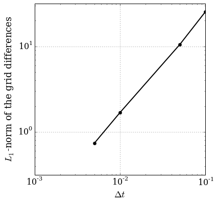
"The symbol $s_m$ is used as it's the *(measured) slope* of the best fit line through the errors, as shown on the [original lesson](http://nbviewer.ipython.org/github/numerical-mooc/numerical-mooc/blob/master/lessons/01_phugoid/01_03_PhugoidFullModel.ipynb):\n",
"\n",
"\n",
"####Figure 1. Convergence test plot taken from the original lesson."
]
},
{
"cell_type": "markdown",
"metadata": {},
"source": [
"The [original lesson](http://nbviewer.ipython.org/github/numerical-mooc/numerical-mooc/blob/master/lessons/01_phugoid/01_03_PhugoidFullModel.ipynb) does precisely this comparison (using the phugoid model, with specific parameter values, and $\\dt = 0.001$), finding a measured slope $s_m = 1.014$. Is this *close enough* to 1?"
]
},
{
"cell_type": "markdown",
"metadata": {},
"source": [
"## TL;DR: Answer"
]
},
{
"cell_type": "markdown",
"metadata": {},
"source": [
"Answer**s**\n",
"\n",
"1. [*I don't care about the algorithm: I just want the answer to be right*](http://nbviewer.ipython.org/github/IanHawke/close-enough-balloons/blob/master/01-Close-Enough-Errorbars.ipynb): $0.585 \\lesssim s_m \\lesssim 1.585$ is close enough for Euler's method.\n",
"2. [*I don't care about the answer: I just want the algorithm behaviour to be right*](http://nbviewer.ipython.org/github/IanHawke/close-enough-balloons/blob/master/02-Close-Enough-Slopes.ipynb): $s_m=1.014$ with $\\dt=0.001$ is close enough if $1 \\le s_m \\le 1.0093$ with $\\dt=0.0005$.\n",
"3. [*I don't care about the behaviour: I just want to know I've implemented Euler's method*](http://nbviewer.ipython.org/github/IanHawke/close-enough-balloons/blob/master/03-Close-Enough-Just-Euler.ipynb): measure the local truncation error instead, and check *both* the convergence rate *and* the leading order constant. $s_m$ by itself is useless."
]
}
],
"metadata": {
"kernelspec": {
"display_name": "Python 3",
"language": "python",
"name": "python3"
},
"language_info": {
"codemirror_mode": {
"name": "ipython",
"version": 3
},
"file_extension": ".py",
"mimetype": "text/x-python",
"name": "python",
"nbconvert_exporter": "python",
"pygments_lexer": "ipython3",
"version": "3.4.2"
}
},
"nbformat": 4,
"nbformat_minor": 0
}