---
title: "Session 1"
author: "T. Evgeniou"
output: html_document
---
**Note:** you can create an html file by running in your console the command:
rmarkdown::render("CourseSessions/Session1/Session1inclass.Rmd")
The purpose of this session is to become familiar with:
1. Basic functionality of R;
2. Reading/Writing data;
3. Simple data manipulations;
4. Simple plots;
4. The idea of functions
Before starting, make sure you have pulled the [session 1 files](https://github.com/InseadDataAnalytics/INSEADAnalytics/tree/master/CourseSessions/Session1) on your github repository (if you pull the course github repository you also get the session files automatically). To confirm, you can also "source" the file "update_fork.R" which you can find in your main course directory.
Note also that directory paths may sometimes be a frustrating source of problems, so it is recommended that you learn these R commands to find out your current working directory and, if needed, set it where you need to (e.g. where you have the main files for the class). For example, assuming we are now in the "MYDIRECTORY/INSEADAnalytics" directory, we can do these:
```{r echo=TRUE, eval=FALSE, tidy=TRUE}
# This command shows the directory we are at (Note: the "#" sign at the begining of a line of code indicates that the line should not be executed - it is a commented out line, so you need to remove the "#" character and then run the line):
# getwd()
# This command can change the directory if we need to:
# setwd("CourseSessions/Session1")
```
Let's start.
**Note:** you can always use the `help` command in Rstudio to find out about any R function (e.g. type `help(list.files)` to learn what the R function `list.files` does).
### Setting up
First, notice the structure of this file when you open it in your RStudio (the "raw file"). This is a so called [Markdown file](http://rmarkdown.rstudio.com/) file (ending with .Rmd). Markdown files are excellent ways to create reproducible, reusable, and easy to modify reports. Effectively one combines text with code within the same file. The code can be inserted either using *code chunks* which, as you can note below, are effectively blocks of code that start for example as:
"```{r eval = TRUE, echo=TRUE, comment=NA, warning=FALSE, message=FALSE,results='markup'}"
or by adding simple code commands in the text like the inline "r colnames(ProjectData)[2]" that you can find further below. When one compiles the file (e.g. using the "rmarkdown::render" command as shown at the beginning of this document) then all code is executed and the output is seamlessly merged within the document.
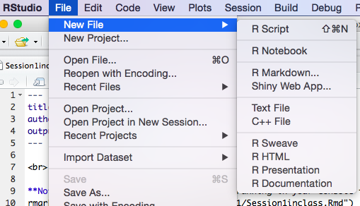
You can create a new .Rmd by creating a new "R Markdown" file as shown in this image:
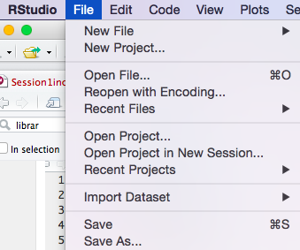
In general once you create any new file, you will be asked to give it a name when you try to save it for the first time:
Markdown (ending at .Rmd) files are not like the usual *R Script* (which end with .R) files. The latter only contain code, such as custom functions we may want to build. Here is an [example .R file](https://github.com/InseadDataAnalytics/INSEADAnalytics/blob/master/CourseSessions/Session1/library.R). One can incorporate such .R files in the .Rmd document by simply "sourcing" these files, like in this example:
```{r eval = FALSE, echo=TRUE, comment=NA, warning=FALSE, message=FALSE,results='asis'}
source("library.R")
```
(note that the directory path is defined relative to where the current .Rmd file is located - in this case they are both in the same directory).
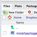
Notice also the [structure of the Session 1 directory](https://github.com/InseadDataAnalytics/INSEADAnalytics/tree/master/CourseSessions/Session1). All it has (other than a few image files) is one .Rmd file, one .R file and one directory where we keep the data (which you can create using the "New Folder" button).
#### Questions
1. Please create a new directory within the "CourseSessions/Session1/" directory (e.g. call this directory "MyProject"), and populate it with a new .Rmd file (e.g. save it as "MyProject.Rmd"), a new .R file (e.g. save it as "library.r"), and a sub-directory (name it "data") where you add a .csv file (for example copy the Boads.csv file from the data directory in Session1).
2. Please add this code chunk in your .Rmd file
```{r eval = TRUE, echo=TRUE, comment=NA, warning=FALSE, message=FALSE,results='markup'}
ProjectData <- read.csv(file = "data/Boats.csv", header = TRUE, sep=",")
ncol(ProjectData)
```
3. What happens when you create an html file (e.g. using the "rmarkdown::render" command but with your new .Rmd filename as argument)?
**Your Answer here:**
### Adding libraries
One of the major benefits of using open source software is the impressive availability of many functions as well as code people develop and share. There is a very fast growing body of (free) tools you can use (also in your jobs) - so avoid reinventing the wheel and ride the wave.
There are many ways to get new tools. First, "mature/tested" tools are available as "packages" that you can install through your RStudio. Take a look at this [list of R packages](https://cran.r-project.org/web/packages/available_packages_by_name.html) and see which ones you like.
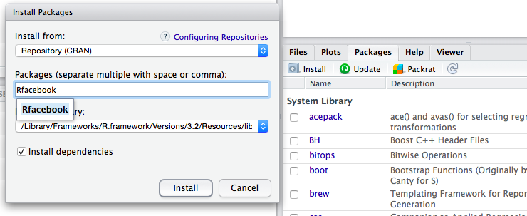
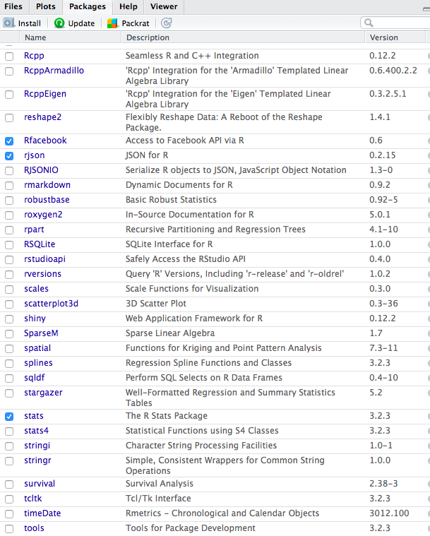
To install a package in R click on the "Packages" menu and then on "Install" and type the name of the package to install, also selecting "Install dependencies", as indicated in this figure:
This will download the package - hence you need to be online. You can then "load" the library by either selecting it in the list of packages you have or using the `library` command in R, for example `library("Rfacebook")`.
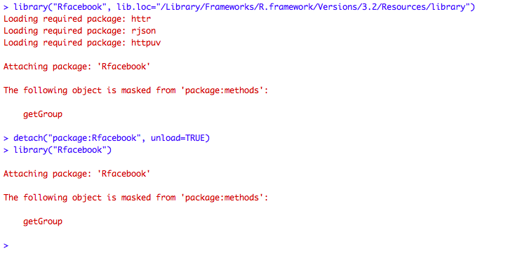
Once you have the library you can click on it (in the "Packages" menu) to see the commands available (also available on the [list of R packages](https://cran.r-project.org/web/packages/available_packages_by_name.html) page, for example in this case for the [Rfacebook documentation).](https://cran.r-project.org/web/packages/Rfacebook/Rfacebook.pdf) You can then explore - always searching the internet for sample code (e.g. for [facebook app examples](http://thinktostart.com/analyzing-facebook-with-r/) or [this](http://blog.revolutionanalytics.com/2013/11/how-to-analyze-you-facebook-friends-network-with-r.html)).
For example you can explore the `RFacebook` library (e.g. start from the `fbOAUth` command and using the [Facebook app id page](https://developers.facebook.com/apps) and the [Facebook app secret](https://developers.facebook.com/apps) pages, then create a token and use it to run commands like these:
```{r eval = FALSE, echo=TRUE, comment=NA, warning=FALSE, message=FALSE,results='asis'}
my_friends <- getFriends(token=token, simplify=TRUE)
my_likes <- getLikes(user="me", token=token)
my_checkins <- getCheckins(user="me", token=token)
my_newsfeed <- getNewsfeed(token=fb_oauth, n=100)
my_network <- getNetwork(token=token, format="adj.matrix")
```
**Note:** Some libraries may require you restart RStudio or install other software or restart your computer.
**Note:** There are efficient ways to install packages. For example one can use something like what we use [in this code.](https://github.com/InseadDataAnalytics/INSEADAnalytics/blob/master/CourseSessions/Sessions23/R/library.R)
### Getting code from Github Repositories
An alternative way to get code (and see sample code - best way to learn) is to simply browse the vast number of public github accounts online. For example this lists some [trending repositories](https://github.com/trending?l=R) (this takes time to be created!) or even the [R language source code itself](https://github.com/wch/r-source) or of course links from many other [resources on R](http://www.r-bloggers.com/tag/github/). Welcome to this new world!
#### Questions
1. Do you have, and if not, can you install these packages? `datasets`, `FactoMineR`,`png` and `stringr`
2. Please find a github repository that you would like to explore and fork it in your github account. Which one did you select?
### Read/Write Data
Let's now read some data. There are many ways to do so, including reading from .csv files using the commands `read.csv` and `write.csv`. The "native" way to read and write R data though is using the `save` and `load` commands.
Let's read some data from a .csv file for now - make sure you pulled the course github repository so that you have all the necessary files including the csv files.
```{r eval = TRUE, echo=TRUE, comment=NA, warning=FALSE, message=FALSE,results='markup'}
ProjectData <- read.csv(file = "data/Boats.csv", header = TRUE, sep=",")
```
Let's see what this data is Run these commands to see the number of rows, number of columns, and names of the rows and the columns:
```{r eval = FALSE, echo=TRUE, comment=NA, warning=FALSE, message=FALSE,results='markup'}
ncol(ProjectData)
colnames(ProjectData)
rownames(ProjectData)
```
Do these look like what you see when you open the .csv file using Excel?
### Data Exploration: A Market Segmentation Case
This data is from the case study ["Boats (A): A Segmentation Case"](http://inseaddataanalytics.github.io/INSEADAnalytics/Boats-A-prerelease.pdf) - you can see the data description in the appendix (of course the data are not the actual business data, but similar in spirit). This is based on an actual project of the company (a leader in the boats market) that did a market segmentation in order to re-define its brand and new product development strategies. Business related information on the project is provided in the [Market Segmentation Case Study slides](http://inseaddataanalytics.github.io/INSEADAnalytics/BoatsSegmentationCaseSlides.pdf). We will develop this segmentation solution step by step using the tools we will discuss in sessions 3-6 - see for example the tools of [sessions 2-3](https://github.com/InseadDataAnalytics/INSEADAnalytics/tree/master/CourseSessions/Sessions23) as well as the readings in sessions 3-6.
Let's start with some simple exploration of this data for now. Let's first get some summary statistics. For example the second column (`r colnames(ProjectData)[2]`) has the following descriptive statistics:
```{r eval = TRUE, echo=TRUE, comment=NA, warning=FALSE, message=FALSE,results='markup'}
print(colnames(ProjectData)[2])
mean(ProjectData[,2])
sd(ProjectData[,2])
range(ProjectData[,2])
min(ProjectData[,2])
max(ProjectData[,2])
quantile(ProjectData[,2],0.1)
quantile(ProjectData[,2],0.5)
quantile(ProjectData[,2],0.9)
summary(ProjectData[,2])
```
and the histogram
```{r eval = TRUE, echo=TRUE, comment=NA, warning=FALSE, message=FALSE,results='markup'}
hist(ProjectData[,2], main = "The second column", xlab = "Ratings", ylab = "Respondents")
```
We can also see how the answers of the respondents to the questions correlate with each other. For example the correlation matrix of the first 10 survey questions is:
```{r eval = TRUE, echo=TRUE, comment=NA, warning=FALSE, message=FALSE,results='markup'}
tmp = ProjectData[,2:10]
colnames(tmp) <- 2:10
print(round(cor(tmp),2))
```
The correlation matrix does not look pretty for now, but we will see example ways to make it nicer looking later (see for example the tables in the readings for [sessions 3-4](http://inseaddataanalytics.github.io/INSEADAnalytics/Report_s23.html)) - there are as usual many ways to make really great visualizations in R, using also Google Charts, see some starting points on the [course website technical resources.](http://inseaddataanalytics.github.io/INSEADAnalytics/TechResources.html)
#### Questions
1. Can you find which column asks about the name of the brand rated?
2. Can you find the average rating to question " `r gsub("_", " ", gsub("\\.", " ", "Q1_3_The.brand.of.boat.I.buy.says.a.lot.about.who.I.am"))` ".
3. Which of the R packages or github repositories you explored did you find interesting?
4. *(Extra)* What is the percentage of male in this population? How many of them responded that they plan to purchase a boat in the future?
5. Finally, once you answer all questions, please commit-then-push to your github (as shown in steps 3-5 of the [Getting Started Instructions](https://github.com/InseadDataAnalytics/INSEADAnalytics/wiki/Getting-Started) document) your file as well as all other files in the new directory you created.
**Your Answers here:**
Once done with this, we can now move to the [main project/document we will use in class](https://github.com/InseadDataAnalytics/INSEADAnalytics/blob/master/CourseSessions/InClassProcess) and make sure you can create an html file from it (see also this [issue](https://github.com/InseadDataAnalytics/INSEADAnalytics/issues/69) if needed).