# geocmeans ## An R package to perform Spatial Fuzzy C-means. [](https://github.com/JeremyGelb/geocmeans/actions/workflows/R-CMD-check.yaml) [](https://github.com/JeremyGelb/geocmeans) [](https://cran.r-project.org/package=geocmeans) [](https://cran.r-project.org/package=geocmeans) [](https://app.codecov.io/gh/JeremyGelb/geocmeans?branch=master) [](https://doi.org/10.5281/zenodo.8316593) The website of the package is available [here](https://jeremygelb.github.io/geocmeans/) ## Breaking news Here we are! We are moving from `maptools`, `sp`, `rgeos`, `raster` and `rgdal` to `sf`, `terra` and `tmap`. All the functions and the documentation were modified accordingly. If you spot an error or a bug, please open an issue on github. ## Installation The stable version of `geocmeans` is available on CRAN. You can install it with the command below. install.packages("geocmeans") You can install a development version of the `geocmeans` package using the command below. remotes::install_github(repo = "JeremyGelb/geocmeans", build_vignettes = TRUE, force = TRUE) ## Authors Jeremy Gelb, Laboratoire d’Équité Environnemental INRS (CANADA), Email: ## Contributors Philippe Apparicio, Laboratoire d’Équité Environnemental INRS (CANADA), Email: ## About the package Provides functions to apply Spatial Fuzzy c-means Algorithm, visualize and interpret results. This method is well suited when the user wants to analyze data with a fuzzy clustering algorithm and to account for the spatial dimension of the dataset. In addition, indexes for measuring the spatial consistency and classification quality are proposed. The algorithms were developed first for brain imagery as described in the articles of [Cai and al. 2007](https://doi.org/10.1016/j.patcog.2006.07.011) and [Zaho and al. 2013](https://doi.org/10.1016/j.dsp.2012.09.016). [Gelb and Apparicio](https://doi.org/10.4000/cybergeo.36414) proposed to apply the method to perform a socio-residential and environmental taxonomy in Lyon (France). The methods can be applied to dataframes or to rasters. #### Fuzzy classification algorithms Four Fuzzy classification algorithms are proposed : - FCM: Fuzzy C-Means, with the function `CMeans` - GFCM: Generalized Fuzzy C-Means, with the function `GFCMeans` - SFCM: Spatial Fuzzy C-Means, with the function `SFCMeans` - SGFCM: Spatial Generalized Fuzzy C-Means, with the function `SGFCMeans` Each function return a membership matrix, the data used for the classification (scaled if required) and the centers of the clusters. For each algorithm, it is possible to calculate a “robust version” and to add a noise group (used to catch outliers). See the parameters `robust` and `noise_cluser` in the documentation for more details. #### Parameter selections The algorithms available require different parameters to be fixed by the user. The function `selectParameters` is a useful tool to compare the results of different combinations of parameters. A multicore version, `selectParameters.mc`, using a plan from the package `future` is also available to speed up the calculus. #### Classification quality Many indices of classification quality can be calculated with the function `calcqualityIndexes`: - *Silhouette.index*: the silhouette index (`fclust::SIL.F`) - *Partition.entropy*: the partition entropy index (`fclust::PE`) - *Partition.coeff*: the partition entropy coefficient (`fclust::PC`) - *Modified.partition.coeff*: the modified partition entropy coefficient (`fclust::MPC`) - *XieBeni.index*: the Xie and Beni index (`fclust::XB`) - *FukuyamaSugeno.index*: the Fukuyama and Sugeno index (`geocmeans::calcFukuyamaSugeno`) - *DavidBoudlin.index*: the David-Bouldin index (`geocmeans::calcDavidBouldin`) - *CalinskiHarabasz.index*: the Calinski-Harabasz index (`geocmeans::calcCalinskiHarabasz`) - *GD43.index* and *GD53.index*: two version of the generalized Dunn index (`geocmeans::calcGD43` and `calcGD53`) - *Negentropy.index*: the Negentropy Increment index (`geocmeans::calcNegentropyI`) - *Explained.inertia*: the percentage of total inertia explained by the solution #### Classification consistency To assess the stability of the obtained clusters, a function for bootstrap validation is proposed: `boot_group_validation`. The results can be used to verify if the obtained clusters are stable and how much their centres vary. #### Reproductibility Clustering methods like CMeans depend on the initial centers selected. In `geocmeans`, they are selected randomly, and two runs of the functions can yield different results. To facilitate the reproductibility of the results, the main functions of the package (`CMeans`, `GFCMeans`, `SFCMeans`, `SGFCMeans`, `selectParameters`, `selectParameters.mc`) have a `seed` parameter. It can be set by the user to ensure that the results of the functions are exactly the same. 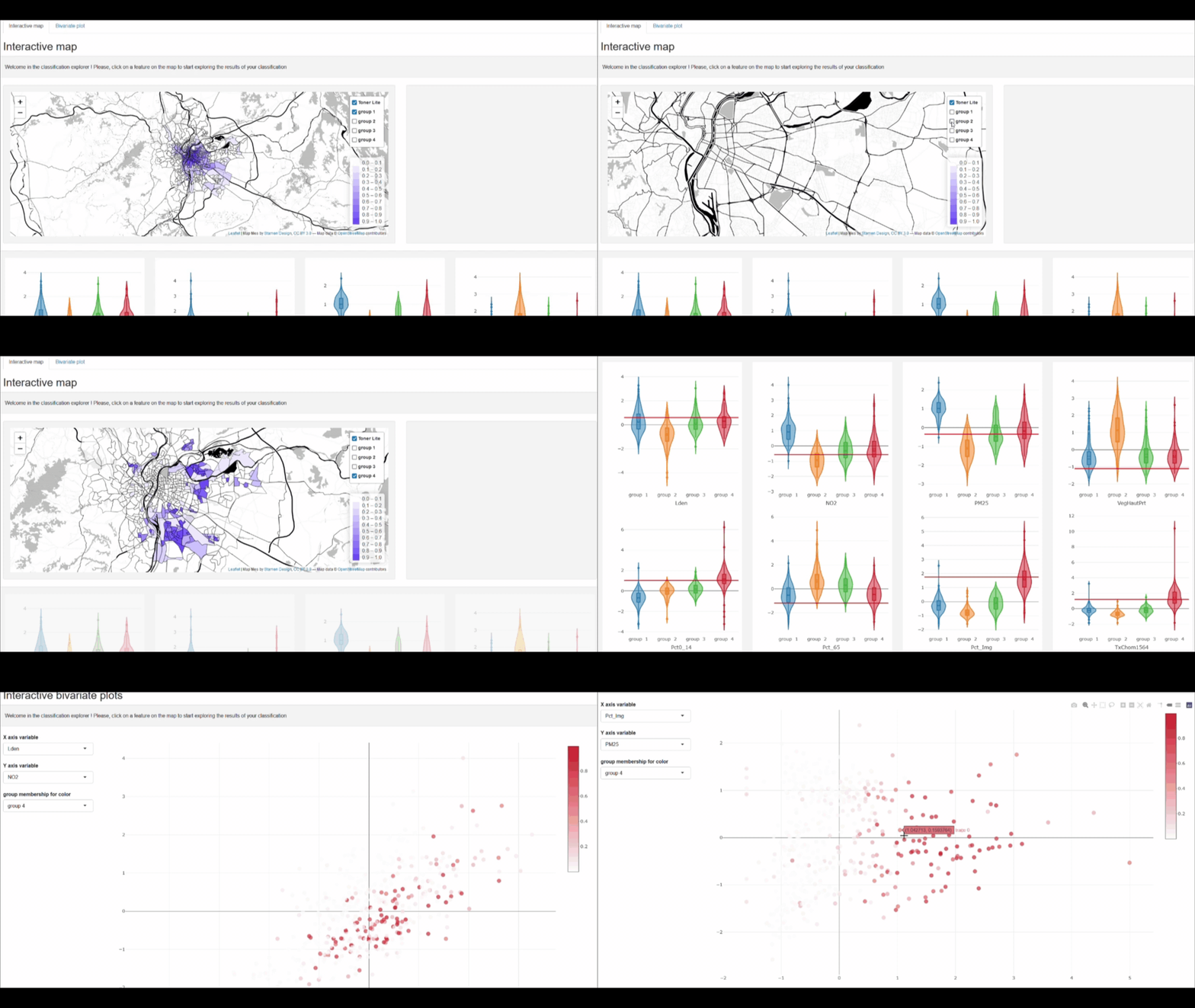#### Interpretation Several functions are also available to facilitate the interpretation of the classification: - summary statistics for each cluster: `summarizeClusters` (also accessible with the generic function `summary`) - spider charts: `spiderPlots` - violin plots: `violinPlots` - maps of the membership matrix: `mapClusters` (support polygon, points and polylines) There is also a shiny app that can be used to go deeper in the result interpretation. It requires the packages `shiny`, `leaflet`, `bslib`, `plotly`, `shinyWidgets`, `car`.

#### Spatial diagnostic Several spatial indices can be calculated to have a better spatial understanding of the obtained clusters, like the global or local Moran I calculated on the membership values, or the join-count-test on the most likely group for each observation. ELSA and Fuzzy ELSA statistics can also be calculated to identify areas with high or low multidimensional spatial autocorrelation in the membership values. See functions `spConsistency`, `calcELSA`, `calcFuzzyELSA` and `spatialDiag`. We proposed an index to quantify the spatial inconsistency of a classification ([Gelb and Apparicio](https://doi.org/10.4000/cybergeo.36414)). If in a classification close observations tend to belong to the same group, then the value of the index is close to 0. If the index is close to 1, then the belonging to groups is randomly distributed in space. A value higher than one can happen in the case of negative spatial autocorrelation. The index is described in the vignette `adjustinconsistency`. The function `spatialDiag` does a complete spatial diagnostic of the membership matrix resulting from a classification. ## Examples Detailed examples are given in the vignette `introduction` vignette("introduction","geocmeans") ## Testing If you would like to install and run the unit tests interactively, include `INSTALL_opts = "--install-tests"` in the installation code. remotes::install_github(repo = "JeremyGelb/geocmeans", build_vignettes = TRUE, force = TRUE, INSTALL_opts = "--install-tests") testthat::test_package("geocmeans", reporter = "stop") ## Contribute To contribute to `geocmeans`, please follow these [guidelines](https://github.com/JeremyGelb/geocmeans/blob/master/CONTRIBUTING.md). Please note that the `geocmeans` project is released with a [Contributor Code of Conduct](https://github.com/JeremyGelb/geocmeans/blob/master/CONDUCT.md). By contributing to this project, you agree to abide by its terms. ## License `geocmeans` version 0.3.4 is licensed under [GPL2 License](https://github.com/JeremyGelb/geocmeans/blob/master/LICENSE.txt).