{
"cells": [
{
"cell_type": "markdown",
"metadata": {
"pycharm": {
"name": "#%% md\n"
}
},
"source": [
"# Lets-Plot Usage Guide\n",
"\n",
"\n",
" \n",
"\n",
"\n",
"\n",
"- [Installation](#install)\n",
"- [Understanding architecture](#implementation)\n",
"- [Learning API](#api)\n",
"- [Getting started](#gsg)\n",
"\n",
"\n",
"**Lets-Plot** is an open-source plotting library for statistical data. It is implemented using the \n",
"[Kotlin programming language](https://kotlinlang.org/) that has a multi-platform nature.\n",
"That's why Lets-Plot provides the plotting functionality that \n",
"is packaged as a JavaScript library, a JVM library, and a native Python extension.\n",
"\n",
"The design of the Lets-Plot library is heavily influenced by [ggplot2](https://ggplot2.tidyverse.org) library.\n",
"\n",
"\n",
"## Installation\n",
"\n",
"Library is distributed via [Maven Central](https://central.sonatype.com/artifact/org.jetbrains.lets-plot/lets-plot-kotlin).\n",
"You can include it in your Kotlin or Java project using Maven or Gradle configuration files (see also [Developer guide](https://github.com/JetBrains/lets-plot-kotlin/blob/master/USAGE_BATIK_JFX_JS.md)),\n",
"or include it in your Jupyter notebook script via `%use lets-plot` annotation (see [Kotlin kernel for IPython/Jupyter](https://github.com/Kotlin/kotlin-jupyter)).\n",
"\n",
"\n",
"## Understanding Lets-Plot architecture\n",
"In `lets-plot`, the **plot** is represented at least by one\n",
"**layer**. It can be built based on the default dataset with the aesthetics mappings, set of scales, or additional \n",
"features applied.\n",
"\n",
"The **Layer** is responsible for creating the objects painted on the ‘canvas’ and it contains the following elements:\n",
"- **Data** - the set of data specified either once for all layers or on a per layer basis.\n",
"One plot can combine multiple different datasets (one per layer).\n",
"- **Aesthetic mapping** - describes how variables in the dataset are mapped to the visual properties of the layer, such as color, shape, size, or position.\n",
"- **Geometric object** - a geometric object that represents a particular type of charts.\n",
"- **Statistical transformation** - computes some kind of statistical summary on the raw input data. \n",
"For example, `bin` statistics is used for histograms and `smooth` is used for regression lines. \n",
"Most stats take additional parameters to specify details of the statistical transformation of data.\n",
"- **Position adjustment** - a method used to compute the final coordinates of geometry. \n",
"Used to build variants of the same `geom` object or to avoid overplotting.\n",
"\n",
"\n",
"\n",
"\n",
"## Learning API\n",
"The typical code fragment that plots a Lets-Plot chart looks as follows:\n",
"\n",
"```\n",
"import org.jetbrains.letsPlot.*\n",
"import org.jetbrains.letsPlot.geom.*\n",
"import org.jetbrains.letsPlot.stat.*\n",
"\n",
"p = letsPlot() \n",
"p + geom(stat=, position=) { }\n",
"```\n",
"\n",
"### Geometric objects `geom`\n",
"\n",
"You can add a new geometric object (or plot layer) by creating it using the `geomXxx()` function and then adding this object to `ggplot`:\n",
"\n",
"```\n",
"p = letsPlot(data=df)\n",
"p + geomPoint()\n",
"```\n",
"\n",
"See the [geom reference](https://lets-plot.org/kotlin/api-reference/-lets--plot--kotlin/org.jetbrains.letsPlot.geom/index.html) for more information about the supported\n",
"geometric objects, their arguments, and default values.\n",
"\n",
"There is also a few `statXxx()` functions which also create a plot layer.\n",
"Occasionally, it feels more naturally to use `statXxx()` instead of `geomXxx()` function to add a new plot layer.\n",
"For example, you might prefer to use `statCount()` instead of `geomBar()`.\n",
"\n",
"See the [stat layer reference](https://lets-plot.org/kotlin/api-reference/-lets--plot--kotlin/org.jetbrains.letsPlot.stat/index.html) for more information about the supported\n",
"stat plot-layer objects, their arguments, and default values.\n",
"\n",
"\n",
"### Collections of plots\n",
"With the [ggbunch()](https://lets-plot.org/kotlin/api-reference/-lets--plot--kotlin/org.jetbrains.letsPlot/ggbunch.html) function, you can\n",
"render a collection of plots:\n",
"\n",
"```\n",
"ggbunch(\n",
" plots = listOf(plot1, plot2),\n",
" regions = listOf(listOf(0, 0, .5, 1), listOf(.5, 0, .5, 1))\n",
") + ggsize(800, 300)\n",
"```\n",
"\n",
"See the [ggbunch.ipynb](https://nbviewer.org/github/JetBrains/lets-plot-docs/blob/master/source/kotlin_examples/cookbook/ggbunch.ipynb)\n",
" example for more information.\n",
"\n",
"### Stat `stat`\n",
"\n",
"Add `stat` as an argument to `geomXxx()` function to define statistical data transformations:\n",
"\n",
"`geomPoint(stat=Stat.count())`\n",
"\n",
"Supported statistical transformations:\n",
"\n",
"- `identity`: leave the data unchanged\n",
"- `count`: calculate the number of points with same x-axis coordinate\n",
"- `bin`: calculate the number of points falling in each of adjacent equally sized ranges along the x-axis\n",
"- `bin2d`: calculate the number of points falling in each of adjacent equal sized rectangles on the plot plane\n",
"- `smooth`: perform smoothing\n",
"- `contour`, `contourFilled`, : calculate contours of 3D data\n",
"- `boxplot`: calculate components of a box plot.\n",
"- `density`, `density2D`, `density2DFilled`: perform a kernel density estimation for 1D and 2D data\n",
"\n",
"See the [stat reference](https://lets-plot.org/kotlin/api-reference/-lets--plot--kotlin/org.jetbrains.letsPlot/-stat/index.html) for more information about the supported\n",
"stat objects, their arguments, and default values.\n",
"\n",
"\n",
"### Aesthetic mappings `mapping`\n",
"With mappings, you can define how variables in dataset are mapped to the visual elements of the chart.\n",
"Add the `{x=< >; y=< >; ...}` closure to `geom`, where:\n",
"- `x`: the dataframe column to map to the x axis. \n",
"- `y`: the dataframe column to map to the y axis.\n",
"- `...`: other visual properties of the chart, such as color, shape, size, or position.\n",
"\n",
"`geom_point() {x = \"cty\"; y = \"hwy\"; color=\"cyl\"}`\n",
"\n",
"### Position adjustment `position`\n",
"\n",
"All layers have a position adjustment that computes the final coordinates of geometry.\n",
"Position adjustment is used to build variances of the same plots and resolve overlapping.\n",
"Override the default settings by using the `position` argument in the `geom` functions:\n",
"\n",
"`geomBar(position=positionFill)`\n",
"\n",
"or\n",
"\n",
"`geomBar(position=positionDodge(width=1.01))`\n",
"\n",
"Available adjustments:\n",
"- `dodge`\n",
"- `jitter`\n",
"- `jitterdodge`\n",
"- `nudge`\n",
"- `identity`\n",
"- `fill`\n",
"- `stack`\n",
"\n",
"See [position functions reference](https://lets-plot.org/kotlin/api-reference/-lets--plot--kotlin/org.jetbrains.letsPlot.pos/index.html)\n",
"for more information about position adjustments.\n",
"\n",
"### Features affecting the entire plot\n",
"\n",
"#### Scales\n",
"\n",
"Enables choosing a reasonable scale for each mapped variable depending on the variable attributes. Override default scales to tweak\n",
"details like the axis labels or legend keys, or to use a completely different translation from data to aesthetic.\n",
"For example, to override the fill color on the histogram:\n",
"\n",
"`p + geomHistogram() + scaleFillContinuous(\"red\", \"green\")`\n",
"\n",
"See the list of the available `scale` methods in the [scale reference](https://lets-plot.org/kotlin/api-reference/-lets--plot--kotlin/org.jetbrains.letsPlot.scale/index.html)\n",
"\n",
"#### Coordinated system\n",
"\n",
"The coordinate system determines how the x and y aesthetics combine to position elements in the plot.\n",
"For example, to override the default X and Y ratio:\n",
"\n",
"`p + coordFixed(ratio=2)`\n",
"\n",
"See the list of the available methods in [coordinates reference](https://lets-plot.org/kotlin/api-reference/-lets--plot--kotlin/org.jetbrains.letsPlot.coord/index.html)\n",
"\n",
"#### Legend\n",
"The axes and legends help users interpret plots.\n",
"Use the `guide` methods or the `guide` argument of the `scale` method to customize the legend.\n",
"For example, to define the number of columns in the legend:\n",
"\n",
"`p + scaleColorDiscrete(guide=guideLegend(ncol=2))`\n",
"\n",
"See more information about the `guideColorbar, guideLegend` functions in the [scale reference](https://lets-plot.org/kotlin/api-reference/-lets--plot--kotlin/org.jetbrains.letsPlot.scale/index.html)\n",
"\n",
"Adjust legend location on plot using the `theme` legendPosition, legendJustification and legendDirection methods, see:\n",
"[theme reference](https://lets-plot.org/kotlin/api-reference/-lets--plot--kotlin/org.jetbrains.letsPlot.themes/index.html)\n",
"\n",
"#### Sampling\n",
"\n",
"Sampling is a special technique of data transformation built into Lets-Plot and it is applied after stat transformation.\n",
"Sampling helps prevents UI freezes and out-of-memory crashes when attempting to plot an excessively large number of geometries.\n",
"By default, the technique applies automatically when the data volume exceeds a certain threshold.\n",
"The `samplingNone` value disables any sampling for the given layer. The sampling methods can be chained together using the + operator.\n",
"\n",
"Available methods:\n",
"- `samplingRandomStratified`: randomly selects points from each group proportionally to the group size but also ensures\n",
"that each group is represented by at least a specified minimum number of points.\n",
"- `samplingRandom`: selects data points at randomly chosen indices without replacement.\n",
"- `samplingPick`: analyses X-values and selects all points which X-values get in the set of first `n` X-values found in the population.\n",
"- `samplingSystematic`: selects data points at evenly distributed indices.\n",
"- `samplingCertexDP`, `samplingVertexVW`: simplifies plotting of polygons.\n",
"There is a choice of two implementation algorithms: Douglas-Peucker (`DP`) and\n",
"Visvalingam-Whyatt (`VW`).\n",
"\n",
"For more details, see the [sampling reference](https://lets-plot.org/kotlin/api-reference/-lets--plot--kotlin/org.jetbrains.letsPlot.sampling/index.html)."
]
},
{
"cell_type": "markdown",
"metadata": {
"pycharm": {
"name": "#%% md\n"
}
},
"source": [
"\n",
"### Getting started\n",
"\n",
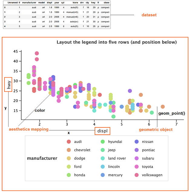
"Let's plot a point chart built using the mpg dataset.\n",
"\n",
"Create the `DataFrame` object and retrieve the data."
]
},
{
"cell_type": "code",
"execution_count": 1,
"metadata": {
"collapsed": false,
"jupyter": {
"outputs_hidden": false
},
"pycharm": {
"is_executing": false,
"name": "#%%\n"
}
},
"outputs": [
{
"data": {
"text/html": [
" \n",
" "
]
},
"metadata": {},
"output_type": "display_data"
},
{
"data": {
"text/html": [
" \n",
" "
]
},
"metadata": {},
"output_type": "display_data"
}
],
"source": [
"%useLatestDescriptors\n",
"%use lets-plot\n",
"@file:DependsOn(\"com.github.doyaaaaaken:kotlin-csv-jvm:0.7.3\")\n",
"\n",
"import com.github.doyaaaaaken.kotlincsv.client.*\n",
"\n",
"val csvData = java.io.File(\"mpg.csv\")\n",
"\n",
"val mpg: List> = CsvReader().readAllWithHeader(csvData)\n",
"\n",
"fun col(name: String, discrete: Boolean=false): List<*> {\n",
" return mpg.map {\n",
" val v = it[name]\n",
" if(discrete) v else v?.toDouble()\n",
" }\n",
"}\n",
"\n",
"val df = mapOf(\n",
" \"displ\" to col(\"displ\"),\n",
" \"hwy\" to col(\"hwy\"),\n",
" \"cyl\" to col(\"cyl\"),\n",
" \"index\" to col(\"\"),\n",
" \"cty\" to col(\"cty\"),\n",
" \"drv\" to col(\"drv\", true),\n",
" \"year\" to col(\"year\")\n",
")"
]
},
{
"cell_type": "markdown",
"metadata": {},
"source": [
"Plot the basic point chart."
]
},
{
"cell_type": "markdown",
"metadata": {},
"source": [
"Perform the following aesthetic mappings:\n",
" - `x` = displ (the **displ** column of the dataframe)\n",
" - `y` = hwy (the **hwy** column of the dataframe)\n",
" - `color` = cyl (the **cyl** column of the dataframe)"
]
},
{
"cell_type": "code",
"execution_count": 2,
"metadata": {
"collapsed": false,
"jupyter": {
"outputs_hidden": false
},
"pycharm": {
"is_executing": false,
"name": "#%%\n"
}
},
"outputs": [
{
"data": {
"text/html": [
" \n",
" "
]
},
"metadata": {},
"output_type": "display_data"
},
{
"data": {
"application/plot+json": {
"apply_color_scheme": true,
"output": {
"data": {
"cty": [
18,
21,
20,
21,
16,
18,
18,
18,
16,
20,
19,
15,
17,
17,
15,
15,
17,
16,
14,
11,
14,
13,
12,
16,
15,
16,
15,
15,
14,
11,
11,
14,
19,
22,
18,
18,
17,
18,
17,
16,
16,
17,
17,
11,
15,
15,
16,
16,
15,
14,
13,
14,
14,
14,
9,
11,
11,
13,
13,
9,
13,
11,
13,
11,
12,
9,
13,
13,
12,
9,
11,
11,
13,
11,
11,
11,
12,
14,
15,
14,
13,
13,
13,
14,
14,
13,
13,
13,
11,
13,
18,
18,
17,
16,
15,
15,
15,
15,
14,
28,
24,
25,
23,
24,
26,
25,
24,
21,
18,
18,
21,
21,
18,
18,
19,
19,
19,
20,
20,
17,
16,
17,
17,
15,
15,
14,
9,
14,
13,
11,
11,
12,
12,
11,
11,
11,
12,
14,
13,
13,
13,
21,
19,
23,
23,
19,
19,
18,
19,
19,
14,
15,
14,
12,
18,
16,
17,
18,
16,
18,
18,
20,
19,
20,
18,
21,
19,
19,
19,
20,
20,
19,
20,
15,
16,
15,
15,
16,
14,
21,
21,
21,
21,
18,
18,
19,
21,
21,
21,
22,
18,
18,
18,
24,
24,
26,
28,
26,
11,
13,
15,
16,
17,
15,
15,
15,
16,
21,
19,
21,
22,
17,
33,
21,
19,
22,
21,
21,
21,
16,
17,
35,
29,
21,
19,
20,
20,
21,
18,
19,
21,
16,
18,
17
],
"cyl": [
4,
4,
4,
4,
6,
6,
6,
4,
4,
4,
4,
6,
6,
6,
6,
6,
6,
8,
8,
8,
8,
8,
8,
8,
8,
8,
8,
8,
8,
8,
8,
8,
4,
4,
6,
6,
6,
4,
6,
6,
6,
6,
6,
6,
6,
6,
6,
6,
6,
6,
6,
6,
8,
8,
8,
8,
8,
6,
8,
8,
8,
8,
8,
8,
8,
8,
8,
8,
8,
8,
8,
8,
8,
8,
8,
8,
8,
6,
6,
6,
6,
8,
8,
6,
6,
8,
8,
8,
8,
8,
6,
6,
6,
6,
8,
8,
8,
8,
8,
4,
4,
4,
4,
4,
4,
4,
4,
4,
4,
4,
4,
4,
6,
6,
6,
4,
4,
4,
4,
6,
6,
6,
6,
6,
6,
8,
8,
8,
8,
8,
8,
8,
8,
8,
8,
8,
8,
6,
6,
8,
8,
4,
4,
4,
4,
6,
6,
6,
6,
6,
6,
6,
6,
8,
6,
6,
6,
6,
8,
4,
4,
4,
4,
4,
4,
4,
4,
4,
4,
4,
4,
4,
4,
4,
4,
6,
6,
6,
8,
4,
4,
4,
4,
6,
6,
6,
4,
4,
4,
4,
6,
6,
6,
4,
4,
4,
4,
4,
8,
8,
4,
4,
4,
6,
6,
6,
6,
4,
4,
4,
4,
6,
4,
4,
4,
4,
4,
5,
5,
6,
6,
4,
4,
4,
4,
5,
5,
4,
4,
4,
4,
6,
6,
6
],
"displ": [
1.8,
1.8,
2,
2,
2.8,
2.8,
3.1,
1.8,
1.8,
2,
2,
2.8,
2.8,
3.1,
3.1,
2.8,
3.1,
4.2,
5.3,
5.3,
5.3,
5.7,
6,
5.7,
5.7,
6.2,
6.2,
7,
5.3,
5.3,
5.7,
6.5,
2.4,
2.4,
3.1,
3.5,
3.6,
2.4,
3,
3.3,
3.3,
3.3,
3.3,
3.3,
3.8,
3.8,
3.8,
4,
3.7,
3.7,
3.9,
3.9,
4.7,
4.7,
4.7,
5.2,
5.2,
3.9,
4.7,
4.7,
4.7,
5.2,
5.7,
5.9,
4.7,
4.7,
4.7,
4.7,
4.7,
4.7,
5.2,
5.2,
5.7,
5.9,
4.6,
5.4,
5.4,
4,
4,
4,
4,
4.6,
5,
4.2,
4.2,
4.6,
4.6,
4.6,
5.4,
5.4,
3.8,
3.8,
4,
4,
4.6,
4.6,
4.6,
4.6,
5.4,
1.6,
1.6,
1.6,
1.6,
1.6,
1.8,
1.8,
1.8,
2,
2.4,
2.4,
2.4,
2.4,
2.5,
2.5,
3.3,
2,
2,
2,
2,
2.7,
2.7,
2.7,
3,
3.7,
4,
4.7,
4.7,
4.7,
5.7,
6.1,
4,
4.2,
4.4,
4.6,
5.4,
5.4,
5.4,
4,
4,
4.6,
5,
2.4,
2.4,
2.5,
2.5,
3.5,
3.5,
3,
3,
3.5,
3.3,
3.3,
4,
5.6,
3.1,
3.8,
3.8,
3.8,
5.3,
2.5,
2.5,
2.5,
2.5,
2.5,
2.5,
2.2,
2.2,
2.5,
2.5,
2.5,
2.5,
2.5,
2.5,
2.7,
2.7,
3.4,
3.4,
4,
4.7,
2.2,
2.2,
2.4,
2.4,
3,
3,
3.5,
2.2,
2.2,
2.4,
2.4,
3,
3,
3.3,
1.8,
1.8,
1.8,
1.8,
1.8,
4.7,
5.7,
2.7,
2.7,
2.7,
3.4,
3.4,
4,
4,
2,
2,
2,
2,
2.8,
1.9,
2,
2,
2,
2,
2.5,
2.5,
2.8,
2.8,
1.9,
1.9,
2,
2,
2.5,
2.5,
1.8,
1.8,
2,
2,
2.8,
2.8,
3.6
],
"drv": [
"f",
"f",
"f",
"f",
"f",
"f",
"f",
"4",
"4",
"4",
"4",
"4",
"4",
"4",
"4",
"4",
"4",
"4",
"r",
"r",
"r",
"r",
"r",
"r",
"r",
"r",
"r",
"r",
"4",
"4",
"4",
"4",
"f",
"f",
"f",
"f",
"f",
"f",
"f",
"f",
"f",
"f",
"f",
"f",
"f",
"f",
"f",
"f",
"4",
"4",
"4",
"4",
"4",
"4",
"4",
"4",
"4",
"4",
"4",
"4",
"4",
"4",
"4",
"4",
"4",
"4",
"4",
"4",
"4",
"4",
"4",
"4",
"4",
"4",
"r",
"r",
"r",
"4",
"4",
"4",
"4",
"4",
"4",
"4",
"4",
"4",
"4",
"4",
"4",
"4",
"r",
"r",
"r",
"r",
"r",
"r",
"r",
"r",
"r",
"f",
"f",
"f",
"f",
"f",
"f",
"f",
"f",
"f",
"f",
"f",
"f",
"f",
"f",
"f",
"f",
"f",
"f",
"f",
"f",
"f",
"f",
"f",
"4",
"4",
"4",
"4",
"4",
"4",
"4",
"4",
"4",
"4",
"4",
"4",
"r",
"r",
"r",
"4",
"4",
"4",
"4",
"f",
"f",
"f",
"f",
"f",
"f",
"f",
"f",
"f",
"4",
"4",
"4",
"4",
"f",
"f",
"f",
"f",
"f",
"4",
"4",
"4",
"4",
"4",
"4",
"4",
"4",
"4",
"4",
"4",
"4",
"4",
"4",
"4",
"4",
"4",
"4",
"4",
"4",
"f",
"f",
"f",
"f",
"f",
"f",
"f",
"f",
"f",
"f",
"f",
"f",
"f",
"f",
"f",
"f",
"f",
"f",
"f",
"4",
"4",
"4",
"4",
"4",
"4",
"4",
"4",
"4",
"f",
"f",
"f",
"f",
"f",
"f",
"f",
"f",
"f",
"f",
"f",
"f",
"f",
"f",
"f",
"f",
"f",
"f",
"f",
"f",
"f",
"f",
"f",
"f",
"f",
"f",
"f"
],
"hwy": [
29,
29,
31,
30,
26,
26,
27,
26,
25,
28,
27,
25,
25,
25,
25,
24,
25,
23,
20,
15,
20,
17,
17,
26,
23,
26,
25,
24,
19,
14,
15,
17,
27,
30,
26,
29,
26,
24,
24,
22,
22,
24,
24,
17,
22,
21,
23,
23,
19,
18,
17,
17,
19,
19,
12,
17,
15,
17,
17,
12,
17,
16,
18,
15,
16,
12,
17,
17,
16,
12,
15,
16,
17,
15,
17,
17,
18,
17,
19,
17,
19,
19,
17,
17,
17,
16,
16,
17,
15,
17,
26,
25,
26,
24,
21,
22,
23,
22,
20,
33,
32,
32,
29,
32,
34,
36,
36,
29,
26,
27,
30,
31,
26,
26,
28,
26,
29,
28,
27,
24,
24,
24,
22,
19,
20,
17,
12,
19,
18,
14,
15,
18,
18,
15,
17,
16,
18,
17,
19,
19,
17,
29,
27,
31,
32,
27,
26,
26,
25,
25,
17,
17,
20,
18,
26,
26,
27,
28,
25,
25,
24,
27,
25,
26,
23,
26,
26,
26,
26,
25,
27,
25,
27,
20,
20,
19,
17,
20,
17,
29,
27,
31,
31,
26,
26,
28,
27,
29,
31,
31,
26,
26,
27,
30,
33,
35,
37,
35,
15,
18,
20,
20,
22,
17,
19,
18,
20,
29,
26,
29,
29,
24,
44,
29,
26,
29,
29,
29,
29,
23,
24,
44,
41,
29,
26,
28,
29,
29,
29,
28,
29,
26,
26,
26
],
"index": [
1,
2,
3,
4,
5,
6,
7,
8,
9,
10,
11,
12,
13,
14,
15,
16,
17,
18,
19,
20,
21,
22,
23,
24,
25,
26,
27,
28,
29,
30,
31,
32,
33,
34,
35,
36,
37,
38,
39,
40,
41,
42,
43,
44,
45,
46,
47,
48,
49,
50,
51,
52,
53,
54,
55,
56,
57,
58,
59,
60,
61,
62,
63,
64,
65,
66,
67,
68,
69,
70,
71,
72,
73,
74,
75,
76,
77,
78,
79,
80,
81,
82,
83,
84,
85,
86,
87,
88,
89,
90,
91,
92,
93,
94,
95,
96,
97,
98,
99,
100,
101,
102,
103,
104,
105,
106,
107,
108,
109,
110,
111,
112,
113,
114,
115,
116,
117,
118,
119,
120,
121,
122,
123,
124,
125,
126,
127,
128,
129,
130,
131,
132,
133,
134,
135,
136,
137,
138,
139,
140,
141,
142,
143,
144,
145,
146,
147,
148,
149,
150,
151,
152,
153,
154,
155,
156,
157,
158,
159,
160,
161,
162,
163,
164,
165,
166,
167,
168,
169,
170,
171,
172,
173,
174,
175,
176,
177,
178,
179,
180,
181,
182,
183,
184,
185,
186,
187,
188,
189,
190,
191,
192,
193,
194,
195,
196,
197,
198,
199,
200,
201,
202,
203,
204,
205,
206,
207,
208,
209,
210,
211,
212,
213,
214,
215,
216,
217,
218,
219,
220,
221,
222,
223,
224,
225,
226,
227,
228,
229,
230,
231,
232,
233,
234
],
"year": [
1999,
1999,
2008,
2008,
1999,
1999,
2008,
1999,
1999,
2008,
2008,
1999,
1999,
2008,
2008,
1999,
2008,
2008,
2008,
2008,
2008,
1999,
2008,
1999,
1999,
2008,
2008,
2008,
2008,
2008,
1999,
1999,
1999,
2008,
1999,
2008,
2008,
1999,
1999,
1999,
1999,
2008,
2008,
2008,
1999,
1999,
2008,
2008,
2008,
2008,
1999,
1999,
2008,
2008,
2008,
1999,
1999,
1999,
2008,
2008,
2008,
1999,
2008,
1999,
2008,
2008,
2008,
2008,
2008,
2008,
1999,
1999,
2008,
1999,
1999,
1999,
2008,
1999,
1999,
1999,
2008,
2008,
1999,
1999,
1999,
1999,
1999,
2008,
1999,
2008,
1999,
1999,
2008,
2008,
1999,
1999,
2008,
2008,
2008,
1999,
1999,
1999,
1999,
1999,
2008,
2008,
2008,
2008,
1999,
1999,
2008,
2008,
1999,
1999,
2008,
1999,
1999,
2008,
2008,
2008,
2008,
2008,
2008,
2008,
1999,
1999,
2008,
2008,
2008,
2008,
1999,
2008,
2008,
1999,
1999,
1999,
2008,
1999,
2008,
2008,
1999,
1999,
1999,
2008,
2008,
2008,
2008,
1999,
1999,
2008,
1999,
1999,
2008,
2008,
1999,
1999,
1999,
2008,
2008,
1999,
1999,
2008,
2008,
2008,
2008,
1999,
1999,
1999,
1999,
2008,
2008,
2008,
2008,
1999,
1999,
1999,
1999,
2008,
2008,
1999,
1999,
2008,
2008,
1999,
1999,
2008,
1999,
1999,
2008,
2008,
1999,
1999,
2008,
1999,
1999,
1999,
2008,
2008,
1999,
2008,
1999,
1999,
2008,
1999,
1999,
2008,
2008,
1999,
1999,
2008,
2008,
1999,
1999,
1999,
1999,
2008,
2008,
2008,
2008,
1999,
1999,
1999,
1999,
1999,
1999,
2008,
2008,
1999,
1999,
2008,
2008,
1999,
1999,
2008
]
},
"data_meta": {
"series_annotations": [
{
"column": "displ",
"type": "float"
},
{
"column": "hwy",
"type": "float"
},
{
"column": "cyl",
"type": "float"
},
{
"column": "index",
"type": "float"
},
{
"column": "cty",
"type": "float"
},
{
"column": "drv",
"type": "str"
},
{
"column": "year",
"type": "float"
}
]
},
"kind": "plot",
"layers": [
{
"data": {
"cty": [
18,
21,
20,
21,
16,
18,
18,
18,
16,
20,
19,
15,
17,
17,
15,
15,
17,
16,
14,
11,
14,
13,
12,
16,
15,
16,
15,
15,
14,
11,
11,
14,
19,
22,
18,
18,
17,
18,
17,
16,
16,
17,
17,
11,
15,
15,
16,
16,
15,
14,
13,
14,
14,
14,
9,
11,
11,
13,
13,
9,
13,
11,
13,
11,
12,
9,
13,
13,
12,
9,
11,
11,
13,
11,
11,
11,
12,
14,
15,
14,
13,
13,
13,
14,
14,
13,
13,
13,
11,
13,
18,
18,
17,
16,
15,
15,
15,
15,
14,
28,
24,
25,
23,
24,
26,
25,
24,
21,
18,
18,
21,
21,
18,
18,
19,
19,
19,
20,
20,
17,
16,
17,
17,
15,
15,
14,
9,
14,
13,
11,
11,
12,
12,
11,
11,
11,
12,
14,
13,
13,
13,
21,
19,
23,
23,
19,
19,
18,
19,
19,
14,
15,
14,
12,
18,
16,
17,
18,
16,
18,
18,
20,
19,
20,
18,
21,
19,
19,
19,
20,
20,
19,
20,
15,
16,
15,
15,
16,
14,
21,
21,
21,
21,
18,
18,
19,
21,
21,
21,
22,
18,
18,
18,
24,
24,
26,
28,
26,
11,
13,
15,
16,
17,
15,
15,
15,
16,
21,
19,
21,
22,
17,
33,
21,
19,
22,
21,
21,
21,
16,
17,
35,
29,
21,
19,
20,
20,
21,
18,
19,
21,
16,
18,
17
],
"cyl": [
4,
4,
4,
4,
6,
6,
6,
4,
4,
4,
4,
6,
6,
6,
6,
6,
6,
8,
8,
8,
8,
8,
8,
8,
8,
8,
8,
8,
8,
8,
8,
8,
4,
4,
6,
6,
6,
4,
6,
6,
6,
6,
6,
6,
6,
6,
6,
6,
6,
6,
6,
6,
8,
8,
8,
8,
8,
6,
8,
8,
8,
8,
8,
8,
8,
8,
8,
8,
8,
8,
8,
8,
8,
8,
8,
8,
8,
6,
6,
6,
6,
8,
8,
6,
6,
8,
8,
8,
8,
8,
6,
6,
6,
6,
8,
8,
8,
8,
8,
4,
4,
4,
4,
4,
4,
4,
4,
4,
4,
4,
4,
4,
6,
6,
6,
4,
4,
4,
4,
6,
6,
6,
6,
6,
6,
8,
8,
8,
8,
8,
8,
8,
8,
8,
8,
8,
8,
6,
6,
8,
8,
4,
4,
4,
4,
6,
6,
6,
6,
6,
6,
6,
6,
8,
6,
6,
6,
6,
8,
4,
4,
4,
4,
4,
4,
4,
4,
4,
4,
4,
4,
4,
4,
4,
4,
6,
6,
6,
8,
4,
4,
4,
4,
6,
6,
6,
4,
4,
4,
4,
6,
6,
6,
4,
4,
4,
4,
4,
8,
8,
4,
4,
4,
6,
6,
6,
6,
4,
4,
4,
4,
6,
4,
4,
4,
4,
4,
5,
5,
6,
6,
4,
4,
4,
4,
5,
5,
4,
4,
4,
4,
6,
6,
6
],
"displ": [
1.8,
1.8,
2,
2,
2.8,
2.8,
3.1,
1.8,
1.8,
2,
2,
2.8,
2.8,
3.1,
3.1,
2.8,
3.1,
4.2,
5.3,
5.3,
5.3,
5.7,
6,
5.7,
5.7,
6.2,
6.2,
7,
5.3,
5.3,
5.7,
6.5,
2.4,
2.4,
3.1,
3.5,
3.6,
2.4,
3,
3.3,
3.3,
3.3,
3.3,
3.3,
3.8,
3.8,
3.8,
4,
3.7,
3.7,
3.9,
3.9,
4.7,
4.7,
4.7,
5.2,
5.2,
3.9,
4.7,
4.7,
4.7,
5.2,
5.7,
5.9,
4.7,
4.7,
4.7,
4.7,
4.7,
4.7,
5.2,
5.2,
5.7,
5.9,
4.6,
5.4,
5.4,
4,
4,
4,
4,
4.6,
5,
4.2,
4.2,
4.6,
4.6,
4.6,
5.4,
5.4,
3.8,
3.8,
4,
4,
4.6,
4.6,
4.6,
4.6,
5.4,
1.6,
1.6,
1.6,
1.6,
1.6,
1.8,
1.8,
1.8,
2,
2.4,
2.4,
2.4,
2.4,
2.5,
2.5,
3.3,
2,
2,
2,
2,
2.7,
2.7,
2.7,
3,
3.7,
4,
4.7,
4.7,
4.7,
5.7,
6.1,
4,
4.2,
4.4,
4.6,
5.4,
5.4,
5.4,
4,
4,
4.6,
5,
2.4,
2.4,
2.5,
2.5,
3.5,
3.5,
3,
3,
3.5,
3.3,
3.3,
4,
5.6,
3.1,
3.8,
3.8,
3.8,
5.3,
2.5,
2.5,
2.5,
2.5,
2.5,
2.5,
2.2,
2.2,
2.5,
2.5,
2.5,
2.5,
2.5,
2.5,
2.7,
2.7,
3.4,
3.4,
4,
4.7,
2.2,
2.2,
2.4,
2.4,
3,
3,
3.5,
2.2,
2.2,
2.4,
2.4,
3,
3,
3.3,
1.8,
1.8,
1.8,
1.8,
1.8,
4.7,
5.7,
2.7,
2.7,
2.7,
3.4,
3.4,
4,
4,
2,
2,
2,
2,
2.8,
1.9,
2,
2,
2,
2,
2.5,
2.5,
2.8,
2.8,
1.9,
1.9,
2,
2,
2.5,
2.5,
1.8,
1.8,
2,
2,
2.8,
2.8,
3.6
],
"drv": [
"f",
"f",
"f",
"f",
"f",
"f",
"f",
"4",
"4",
"4",
"4",
"4",
"4",
"4",
"4",
"4",
"4",
"4",
"r",
"r",
"r",
"r",
"r",
"r",
"r",
"r",
"r",
"r",
"4",
"4",
"4",
"4",
"f",
"f",
"f",
"f",
"f",
"f",
"f",
"f",
"f",
"f",
"f",
"f",
"f",
"f",
"f",
"f",
"4",
"4",
"4",
"4",
"4",
"4",
"4",
"4",
"4",
"4",
"4",
"4",
"4",
"4",
"4",
"4",
"4",
"4",
"4",
"4",
"4",
"4",
"4",
"4",
"4",
"4",
"r",
"r",
"r",
"4",
"4",
"4",
"4",
"4",
"4",
"4",
"4",
"4",
"4",
"4",
"4",
"4",
"r",
"r",
"r",
"r",
"r",
"r",
"r",
"r",
"r",
"f",
"f",
"f",
"f",
"f",
"f",
"f",
"f",
"f",
"f",
"f",
"f",
"f",
"f",
"f",
"f",
"f",
"f",
"f",
"f",
"f",
"f",
"f",
"4",
"4",
"4",
"4",
"4",
"4",
"4",
"4",
"4",
"4",
"4",
"4",
"r",
"r",
"r",
"4",
"4",
"4",
"4",
"f",
"f",
"f",
"f",
"f",
"f",
"f",
"f",
"f",
"4",
"4",
"4",
"4",
"f",
"f",
"f",
"f",
"f",
"4",
"4",
"4",
"4",
"4",
"4",
"4",
"4",
"4",
"4",
"4",
"4",
"4",
"4",
"4",
"4",
"4",
"4",
"4",
"4",
"f",
"f",
"f",
"f",
"f",
"f",
"f",
"f",
"f",
"f",
"f",
"f",
"f",
"f",
"f",
"f",
"f",
"f",
"f",
"4",
"4",
"4",
"4",
"4",
"4",
"4",
"4",
"4",
"f",
"f",
"f",
"f",
"f",
"f",
"f",
"f",
"f",
"f",
"f",
"f",
"f",
"f",
"f",
"f",
"f",
"f",
"f",
"f",
"f",
"f",
"f",
"f",
"f",
"f",
"f"
],
"hwy": [
29,
29,
31,
30,
26,
26,
27,
26,
25,
28,
27,
25,
25,
25,
25,
24,
25,
23,
20,
15,
20,
17,
17,
26,
23,
26,
25,
24,
19,
14,
15,
17,
27,
30,
26,
29,
26,
24,
24,
22,
22,
24,
24,
17,
22,
21,
23,
23,
19,
18,
17,
17,
19,
19,
12,
17,
15,
17,
17,
12,
17,
16,
18,
15,
16,
12,
17,
17,
16,
12,
15,
16,
17,
15,
17,
17,
18,
17,
19,
17,
19,
19,
17,
17,
17,
16,
16,
17,
15,
17,
26,
25,
26,
24,
21,
22,
23,
22,
20,
33,
32,
32,
29,
32,
34,
36,
36,
29,
26,
27,
30,
31,
26,
26,
28,
26,
29,
28,
27,
24,
24,
24,
22,
19,
20,
17,
12,
19,
18,
14,
15,
18,
18,
15,
17,
16,
18,
17,
19,
19,
17,
29,
27,
31,
32,
27,
26,
26,
25,
25,
17,
17,
20,
18,
26,
26,
27,
28,
25,
25,
24,
27,
25,
26,
23,
26,
26,
26,
26,
25,
27,
25,
27,
20,
20,
19,
17,
20,
17,
29,
27,
31,
31,
26,
26,
28,
27,
29,
31,
31,
26,
26,
27,
30,
33,
35,
37,
35,
15,
18,
20,
20,
22,
17,
19,
18,
20,
29,
26,
29,
29,
24,
44,
29,
26,
29,
29,
29,
29,
23,
24,
44,
41,
29,
26,
28,
29,
29,
29,
28,
29,
26,
26,
26
],
"index": [
1,
2,
3,
4,
5,
6,
7,
8,
9,
10,
11,
12,
13,
14,
15,
16,
17,
18,
19,
20,
21,
22,
23,
24,
25,
26,
27,
28,
29,
30,
31,
32,
33,
34,
35,
36,
37,
38,
39,
40,
41,
42,
43,
44,
45,
46,
47,
48,
49,
50,
51,
52,
53,
54,
55,
56,
57,
58,
59,
60,
61,
62,
63,
64,
65,
66,
67,
68,
69,
70,
71,
72,
73,
74,
75,
76,
77,
78,
79,
80,
81,
82,
83,
84,
85,
86,
87,
88,
89,
90,
91,
92,
93,
94,
95,
96,
97,
98,
99,
100,
101,
102,
103,
104,
105,
106,
107,
108,
109,
110,
111,
112,
113,
114,
115,
116,
117,
118,
119,
120,
121,
122,
123,
124,
125,
126,
127,
128,
129,
130,
131,
132,
133,
134,
135,
136,
137,
138,
139,
140,
141,
142,
143,
144,
145,
146,
147,
148,
149,
150,
151,
152,
153,
154,
155,
156,
157,
158,
159,
160,
161,
162,
163,
164,
165,
166,
167,
168,
169,
170,
171,
172,
173,
174,
175,
176,
177,
178,
179,
180,
181,
182,
183,
184,
185,
186,
187,
188,
189,
190,
191,
192,
193,
194,
195,
196,
197,
198,
199,
200,
201,
202,
203,
204,
205,
206,
207,
208,
209,
210,
211,
212,
213,
214,
215,
216,
217,
218,
219,
220,
221,
222,
223,
224,
225,
226,
227,
228,
229,
230,
231,
232,
233,
234
],
"year": [
1999,
1999,
2008,
2008,
1999,
1999,
2008,
1999,
1999,
2008,
2008,
1999,
1999,
2008,
2008,
1999,
2008,
2008,
2008,
2008,
2008,
1999,
2008,
1999,
1999,
2008,
2008,
2008,
2008,
2008,
1999,
1999,
1999,
2008,
1999,
2008,
2008,
1999,
1999,
1999,
1999,
2008,
2008,
2008,
1999,
1999,
2008,
2008,
2008,
2008,
1999,
1999,
2008,
2008,
2008,
1999,
1999,
1999,
2008,
2008,
2008,
1999,
2008,
1999,
2008,
2008,
2008,
2008,
2008,
2008,
1999,
1999,
2008,
1999,
1999,
1999,
2008,
1999,
1999,
1999,
2008,
2008,
1999,
1999,
1999,
1999,
1999,
2008,
1999,
2008,
1999,
1999,
2008,
2008,
1999,
1999,
2008,
2008,
2008,
1999,
1999,
1999,
1999,
1999,
2008,
2008,
2008,
2008,
1999,
1999,
2008,
2008,
1999,
1999,
2008,
1999,
1999,
2008,
2008,
2008,
2008,
2008,
2008,
2008,
1999,
1999,
2008,
2008,
2008,
2008,
1999,
2008,
2008,
1999,
1999,
1999,
2008,
1999,
2008,
2008,
1999,
1999,
1999,
2008,
2008,
2008,
2008,
1999,
1999,
2008,
1999,
1999,
2008,
2008,
1999,
1999,
1999,
2008,
2008,
1999,
1999,
2008,
2008,
2008,
2008,
1999,
1999,
1999,
1999,
2008,
2008,
2008,
2008,
1999,
1999,
1999,
1999,
2008,
2008,
1999,
1999,
2008,
2008,
1999,
1999,
2008,
1999,
1999,
2008,
2008,
1999,
1999,
2008,
1999,
1999,
1999,
2008,
2008,
1999,
2008,
1999,
1999,
2008,
1999,
1999,
2008,
2008,
1999,
1999,
2008,
2008,
1999,
1999,
1999,
1999,
2008,
2008,
2008,
2008,
1999,
1999,
1999,
1999,
1999,
1999,
2008,
2008,
1999,
1999,
2008,
2008,
1999,
1999,
2008
]
},
"data_meta": {
"series_annotations": [
{
"column": "displ",
"type": "float"
},
{
"column": "hwy",
"type": "float"
},
{
"column": "cyl",
"type": "float"
},
{
"column": "index",
"type": "float"
},
{
"column": "cty",
"type": "float"
},
{
"column": "drv",
"type": "str"
},
{
"column": "year",
"type": "float"
}
]
},
"geom": "point",
"mapping": {},
"position": "identity",
"stat": "identity"
}
],
"mapping": {
"color": "cyl",
"x": "displ",
"y": "hwy"
},
"scales": []
},
"output_type": "lets_plot_spec",
"swing_enabled": true
},
"text/html": [
" \n",
" \n",
" "
]
},
"execution_count": 2,
"metadata": {},
"output_type": "execute_result"
}
],
"source": [
"// Mapping\n",
"letsPlot(df) {x = \"displ\"; y = \"hwy\"; color = \"cyl\"} + geomPoint(df)"
]
},
{
"cell_type": "markdown",
"metadata": {},
"source": [
"Apply statistical data transformation to count the number of cases at each x position."
]
},
{
"cell_type": "code",
"execution_count": 3,
"metadata": {
"collapsed": false,
"jupyter": {
"outputs_hidden": false
},
"pycharm": {
"is_executing": false,
"name": "#%%\n"
}
},
"outputs": [
{
"data": {
"application/plot+json": {
"apply_color_scheme": true,
"output": {
"data": {
"cty": [
18,
21,
20,
21,
16,
18,
18,
18,
16,
20,
19,
15,
17,
17,
15,
15,
17,
16,
14,
11,
14,
13,
12,
16,
15,
16,
15,
15,
14,
11,
11,
14,
19,
22,
18,
18,
17,
18,
17,
16,
16,
17,
17,
11,
15,
15,
16,
16,
15,
14,
13,
14,
14,
14,
9,
11,
11,
13,
13,
9,
13,
11,
13,
11,
12,
9,
13,
13,
12,
9,
11,
11,
13,
11,
11,
11,
12,
14,
15,
14,
13,
13,
13,
14,
14,
13,
13,
13,
11,
13,
18,
18,
17,
16,
15,
15,
15,
15,
14,
28,
24,
25,
23,
24,
26,
25,
24,
21,
18,
18,
21,
21,
18,
18,
19,
19,
19,
20,
20,
17,
16,
17,
17,
15,
15,
14,
9,
14,
13,
11,
11,
12,
12,
11,
11,
11,
12,
14,
13,
13,
13,
21,
19,
23,
23,
19,
19,
18,
19,
19,
14,
15,
14,
12,
18,
16,
17,
18,
16,
18,
18,
20,
19,
20,
18,
21,
19,
19,
19,
20,
20,
19,
20,
15,
16,
15,
15,
16,
14,
21,
21,
21,
21,
18,
18,
19,
21,
21,
21,
22,
18,
18,
18,
24,
24,
26,
28,
26,
11,
13,
15,
16,
17,
15,
15,
15,
16,
21,
19,
21,
22,
17,
33,
21,
19,
22,
21,
21,
21,
16,
17,
35,
29,
21,
19,
20,
20,
21,
18,
19,
21,
16,
18,
17
],
"cyl": [
4,
4,
4,
4,
6,
6,
6,
4,
4,
4,
4,
6,
6,
6,
6,
6,
6,
8,
8,
8,
8,
8,
8,
8,
8,
8,
8,
8,
8,
8,
8,
8,
4,
4,
6,
6,
6,
4,
6,
6,
6,
6,
6,
6,
6,
6,
6,
6,
6,
6,
6,
6,
8,
8,
8,
8,
8,
6,
8,
8,
8,
8,
8,
8,
8,
8,
8,
8,
8,
8,
8,
8,
8,
8,
8,
8,
8,
6,
6,
6,
6,
8,
8,
6,
6,
8,
8,
8,
8,
8,
6,
6,
6,
6,
8,
8,
8,
8,
8,
4,
4,
4,
4,
4,
4,
4,
4,
4,
4,
4,
4,
4,
6,
6,
6,
4,
4,
4,
4,
6,
6,
6,
6,
6,
6,
8,
8,
8,
8,
8,
8,
8,
8,
8,
8,
8,
8,
6,
6,
8,
8,
4,
4,
4,
4,
6,
6,
6,
6,
6,
6,
6,
6,
8,
6,
6,
6,
6,
8,
4,
4,
4,
4,
4,
4,
4,
4,
4,
4,
4,
4,
4,
4,
4,
4,
6,
6,
6,
8,
4,
4,
4,
4,
6,
6,
6,
4,
4,
4,
4,
6,
6,
6,
4,
4,
4,
4,
4,
8,
8,
4,
4,
4,
6,
6,
6,
6,
4,
4,
4,
4,
6,
4,
4,
4,
4,
4,
5,
5,
6,
6,
4,
4,
4,
4,
5,
5,
4,
4,
4,
4,
6,
6,
6
],
"displ": [
1.8,
1.8,
2,
2,
2.8,
2.8,
3.1,
1.8,
1.8,
2,
2,
2.8,
2.8,
3.1,
3.1,
2.8,
3.1,
4.2,
5.3,
5.3,
5.3,
5.7,
6,
5.7,
5.7,
6.2,
6.2,
7,
5.3,
5.3,
5.7,
6.5,
2.4,
2.4,
3.1,
3.5,
3.6,
2.4,
3,
3.3,
3.3,
3.3,
3.3,
3.3,
3.8,
3.8,
3.8,
4,
3.7,
3.7,
3.9,
3.9,
4.7,
4.7,
4.7,
5.2,
5.2,
3.9,
4.7,
4.7,
4.7,
5.2,
5.7,
5.9,
4.7,
4.7,
4.7,
4.7,
4.7,
4.7,
5.2,
5.2,
5.7,
5.9,
4.6,
5.4,
5.4,
4,
4,
4,
4,
4.6,
5,
4.2,
4.2,
4.6,
4.6,
4.6,
5.4,
5.4,
3.8,
3.8,
4,
4,
4.6,
4.6,
4.6,
4.6,
5.4,
1.6,
1.6,
1.6,
1.6,
1.6,
1.8,
1.8,
1.8,
2,
2.4,
2.4,
2.4,
2.4,
2.5,
2.5,
3.3,
2,
2,
2,
2,
2.7,
2.7,
2.7,
3,
3.7,
4,
4.7,
4.7,
4.7,
5.7,
6.1,
4,
4.2,
4.4,
4.6,
5.4,
5.4,
5.4,
4,
4,
4.6,
5,
2.4,
2.4,
2.5,
2.5,
3.5,
3.5,
3,
3,
3.5,
3.3,
3.3,
4,
5.6,
3.1,
3.8,
3.8,
3.8,
5.3,
2.5,
2.5,
2.5,
2.5,
2.5,
2.5,
2.2,
2.2,
2.5,
2.5,
2.5,
2.5,
2.5,
2.5,
2.7,
2.7,
3.4,
3.4,
4,
4.7,
2.2,
2.2,
2.4,
2.4,
3,
3,
3.5,
2.2,
2.2,
2.4,
2.4,
3,
3,
3.3,
1.8,
1.8,
1.8,
1.8,
1.8,
4.7,
5.7,
2.7,
2.7,
2.7,
3.4,
3.4,
4,
4,
2,
2,
2,
2,
2.8,
1.9,
2,
2,
2,
2,
2.5,
2.5,
2.8,
2.8,
1.9,
1.9,
2,
2,
2.5,
2.5,
1.8,
1.8,
2,
2,
2.8,
2.8,
3.6
],
"drv": [
"f",
"f",
"f",
"f",
"f",
"f",
"f",
"4",
"4",
"4",
"4",
"4",
"4",
"4",
"4",
"4",
"4",
"4",
"r",
"r",
"r",
"r",
"r",
"r",
"r",
"r",
"r",
"r",
"4",
"4",
"4",
"4",
"f",
"f",
"f",
"f",
"f",
"f",
"f",
"f",
"f",
"f",
"f",
"f",
"f",
"f",
"f",
"f",
"4",
"4",
"4",
"4",
"4",
"4",
"4",
"4",
"4",
"4",
"4",
"4",
"4",
"4",
"4",
"4",
"4",
"4",
"4",
"4",
"4",
"4",
"4",
"4",
"4",
"4",
"r",
"r",
"r",
"4",
"4",
"4",
"4",
"4",
"4",
"4",
"4",
"4",
"4",
"4",
"4",
"4",
"r",
"r",
"r",
"r",
"r",
"r",
"r",
"r",
"r",
"f",
"f",
"f",
"f",
"f",
"f",
"f",
"f",
"f",
"f",
"f",
"f",
"f",
"f",
"f",
"f",
"f",
"f",
"f",
"f",
"f",
"f",
"f",
"4",
"4",
"4",
"4",
"4",
"4",
"4",
"4",
"4",
"4",
"4",
"4",
"r",
"r",
"r",
"4",
"4",
"4",
"4",
"f",
"f",
"f",
"f",
"f",
"f",
"f",
"f",
"f",
"4",
"4",
"4",
"4",
"f",
"f",
"f",
"f",
"f",
"4",
"4",
"4",
"4",
"4",
"4",
"4",
"4",
"4",
"4",
"4",
"4",
"4",
"4",
"4",
"4",
"4",
"4",
"4",
"4",
"f",
"f",
"f",
"f",
"f",
"f",
"f",
"f",
"f",
"f",
"f",
"f",
"f",
"f",
"f",
"f",
"f",
"f",
"f",
"4",
"4",
"4",
"4",
"4",
"4",
"4",
"4",
"4",
"f",
"f",
"f",
"f",
"f",
"f",
"f",
"f",
"f",
"f",
"f",
"f",
"f",
"f",
"f",
"f",
"f",
"f",
"f",
"f",
"f",
"f",
"f",
"f",
"f",
"f",
"f"
],
"hwy": [
29,
29,
31,
30,
26,
26,
27,
26,
25,
28,
27,
25,
25,
25,
25,
24,
25,
23,
20,
15,
20,
17,
17,
26,
23,
26,
25,
24,
19,
14,
15,
17,
27,
30,
26,
29,
26,
24,
24,
22,
22,
24,
24,
17,
22,
21,
23,
23,
19,
18,
17,
17,
19,
19,
12,
17,
15,
17,
17,
12,
17,
16,
18,
15,
16,
12,
17,
17,
16,
12,
15,
16,
17,
15,
17,
17,
18,
17,
19,
17,
19,
19,
17,
17,
17,
16,
16,
17,
15,
17,
26,
25,
26,
24,
21,
22,
23,
22,
20,
33,
32,
32,
29,
32,
34,
36,
36,
29,
26,
27,
30,
31,
26,
26,
28,
26,
29,
28,
27,
24,
24,
24,
22,
19,
20,
17,
12,
19,
18,
14,
15,
18,
18,
15,
17,
16,
18,
17,
19,
19,
17,
29,
27,
31,
32,
27,
26,
26,
25,
25,
17,
17,
20,
18,
26,
26,
27,
28,
25,
25,
24,
27,
25,
26,
23,
26,
26,
26,
26,
25,
27,
25,
27,
20,
20,
19,
17,
20,
17,
29,
27,
31,
31,
26,
26,
28,
27,
29,
31,
31,
26,
26,
27,
30,
33,
35,
37,
35,
15,
18,
20,
20,
22,
17,
19,
18,
20,
29,
26,
29,
29,
24,
44,
29,
26,
29,
29,
29,
29,
23,
24,
44,
41,
29,
26,
28,
29,
29,
29,
28,
29,
26,
26,
26
],
"index": [
1,
2,
3,
4,
5,
6,
7,
8,
9,
10,
11,
12,
13,
14,
15,
16,
17,
18,
19,
20,
21,
22,
23,
24,
25,
26,
27,
28,
29,
30,
31,
32,
33,
34,
35,
36,
37,
38,
39,
40,
41,
42,
43,
44,
45,
46,
47,
48,
49,
50,
51,
52,
53,
54,
55,
56,
57,
58,
59,
60,
61,
62,
63,
64,
65,
66,
67,
68,
69,
70,
71,
72,
73,
74,
75,
76,
77,
78,
79,
80,
81,
82,
83,
84,
85,
86,
87,
88,
89,
90,
91,
92,
93,
94,
95,
96,
97,
98,
99,
100,
101,
102,
103,
104,
105,
106,
107,
108,
109,
110,
111,
112,
113,
114,
115,
116,
117,
118,
119,
120,
121,
122,
123,
124,
125,
126,
127,
128,
129,
130,
131,
132,
133,
134,
135,
136,
137,
138,
139,
140,
141,
142,
143,
144,
145,
146,
147,
148,
149,
150,
151,
152,
153,
154,
155,
156,
157,
158,
159,
160,
161,
162,
163,
164,
165,
166,
167,
168,
169,
170,
171,
172,
173,
174,
175,
176,
177,
178,
179,
180,
181,
182,
183,
184,
185,
186,
187,
188,
189,
190,
191,
192,
193,
194,
195,
196,
197,
198,
199,
200,
201,
202,
203,
204,
205,
206,
207,
208,
209,
210,
211,
212,
213,
214,
215,
216,
217,
218,
219,
220,
221,
222,
223,
224,
225,
226,
227,
228,
229,
230,
231,
232,
233,
234
],
"year": [
1999,
1999,
2008,
2008,
1999,
1999,
2008,
1999,
1999,
2008,
2008,
1999,
1999,
2008,
2008,
1999,
2008,
2008,
2008,
2008,
2008,
1999,
2008,
1999,
1999,
2008,
2008,
2008,
2008,
2008,
1999,
1999,
1999,
2008,
1999,
2008,
2008,
1999,
1999,
1999,
1999,
2008,
2008,
2008,
1999,
1999,
2008,
2008,
2008,
2008,
1999,
1999,
2008,
2008,
2008,
1999,
1999,
1999,
2008,
2008,
2008,
1999,
2008,
1999,
2008,
2008,
2008,
2008,
2008,
2008,
1999,
1999,
2008,
1999,
1999,
1999,
2008,
1999,
1999,
1999,
2008,
2008,
1999,
1999,
1999,
1999,
1999,
2008,
1999,
2008,
1999,
1999,
2008,
2008,
1999,
1999,
2008,
2008,
2008,
1999,
1999,
1999,
1999,
1999,
2008,
2008,
2008,
2008,
1999,
1999,
2008,
2008,
1999,
1999,
2008,
1999,
1999,
2008,
2008,
2008,
2008,
2008,
2008,
2008,
1999,
1999,
2008,
2008,
2008,
2008,
1999,
2008,
2008,
1999,
1999,
1999,
2008,
1999,
2008,
2008,
1999,
1999,
1999,
2008,
2008,
2008,
2008,
1999,
1999,
2008,
1999,
1999,
2008,
2008,
1999,
1999,
1999,
2008,
2008,
1999,
1999,
2008,
2008,
2008,
2008,
1999,
1999,
1999,
1999,
2008,
2008,
2008,
2008,
1999,
1999,
1999,
1999,
2008,
2008,
1999,
1999,
2008,
2008,
1999,
1999,
2008,
1999,
1999,
2008,
2008,
1999,
1999,
2008,
1999,
1999,
1999,
2008,
2008,
1999,
2008,
1999,
1999,
2008,
1999,
1999,
2008,
2008,
1999,
1999,
2008,
2008,
1999,
1999,
1999,
1999,
2008,
2008,
2008,
2008,
1999,
1999,
1999,
1999,
1999,
1999,
2008,
2008,
1999,
1999,
2008,
2008,
1999,
1999,
2008
]
},
"data_meta": {
"series_annotations": [
{
"column": "displ",
"type": "float"
},
{
"column": "hwy",
"type": "float"
},
{
"column": "cyl",
"type": "float"
},
{
"column": "index",
"type": "float"
},
{
"column": "cty",
"type": "float"
},
{
"column": "drv",
"type": "str"
},
{
"column": "year",
"type": "float"
}
]
},
"kind": "plot",
"layers": [
{
"data": {
"cty": [
18,
21,
20,
21,
16,
18,
18,
18,
16,
20,
19,
15,
17,
17,
15,
15,
17,
16,
14,
11,
14,
13,
12,
16,
15,
16,
15,
15,
14,
11,
11,
14,
19,
22,
18,
18,
17,
18,
17,
16,
16,
17,
17,
11,
15,
15,
16,
16,
15,
14,
13,
14,
14,
14,
9,
11,
11,
13,
13,
9,
13,
11,
13,
11,
12,
9,
13,
13,
12,
9,
11,
11,
13,
11,
11,
11,
12,
14,
15,
14,
13,
13,
13,
14,
14,
13,
13,
13,
11,
13,
18,
18,
17,
16,
15,
15,
15,
15,
14,
28,
24,
25,
23,
24,
26,
25,
24,
21,
18,
18,
21,
21,
18,
18,
19,
19,
19,
20,
20,
17,
16,
17,
17,
15,
15,
14,
9,
14,
13,
11,
11,
12,
12,
11,
11,
11,
12,
14,
13,
13,
13,
21,
19,
23,
23,
19,
19,
18,
19,
19,
14,
15,
14,
12,
18,
16,
17,
18,
16,
18,
18,
20,
19,
20,
18,
21,
19,
19,
19,
20,
20,
19,
20,
15,
16,
15,
15,
16,
14,
21,
21,
21,
21,
18,
18,
19,
21,
21,
21,
22,
18,
18,
18,
24,
24,
26,
28,
26,
11,
13,
15,
16,
17,
15,
15,
15,
16,
21,
19,
21,
22,
17,
33,
21,
19,
22,
21,
21,
21,
16,
17,
35,
29,
21,
19,
20,
20,
21,
18,
19,
21,
16,
18,
17
],
"cyl": [
4,
4,
4,
4,
6,
6,
6,
4,
4,
4,
4,
6,
6,
6,
6,
6,
6,
8,
8,
8,
8,
8,
8,
8,
8,
8,
8,
8,
8,
8,
8,
8,
4,
4,
6,
6,
6,
4,
6,
6,
6,
6,
6,
6,
6,
6,
6,
6,
6,
6,
6,
6,
8,
8,
8,
8,
8,
6,
8,
8,
8,
8,
8,
8,
8,
8,
8,
8,
8,
8,
8,
8,
8,
8,
8,
8,
8,
6,
6,
6,
6,
8,
8,
6,
6,
8,
8,
8,
8,
8,
6,
6,
6,
6,
8,
8,
8,
8,
8,
4,
4,
4,
4,
4,
4,
4,
4,
4,
4,
4,
4,
4,
6,
6,
6,
4,
4,
4,
4,
6,
6,
6,
6,
6,
6,
8,
8,
8,
8,
8,
8,
8,
8,
8,
8,
8,
8,
6,
6,
8,
8,
4,
4,
4,
4,
6,
6,
6,
6,
6,
6,
6,
6,
8,
6,
6,
6,
6,
8,
4,
4,
4,
4,
4,
4,
4,
4,
4,
4,
4,
4,
4,
4,
4,
4,
6,
6,
6,
8,
4,
4,
4,
4,
6,
6,
6,
4,
4,
4,
4,
6,
6,
6,
4,
4,
4,
4,
4,
8,
8,
4,
4,
4,
6,
6,
6,
6,
4,
4,
4,
4,
6,
4,
4,
4,
4,
4,
5,
5,
6,
6,
4,
4,
4,
4,
5,
5,
4,
4,
4,
4,
6,
6,
6
],
"displ": [
1.8,
1.8,
2,
2,
2.8,
2.8,
3.1,
1.8,
1.8,
2,
2,
2.8,
2.8,
3.1,
3.1,
2.8,
3.1,
4.2,
5.3,
5.3,
5.3,
5.7,
6,
5.7,
5.7,
6.2,
6.2,
7,
5.3,
5.3,
5.7,
6.5,
2.4,
2.4,
3.1,
3.5,
3.6,
2.4,
3,
3.3,
3.3,
3.3,
3.3,
3.3,
3.8,
3.8,
3.8,
4,
3.7,
3.7,
3.9,
3.9,
4.7,
4.7,
4.7,
5.2,
5.2,
3.9,
4.7,
4.7,
4.7,
5.2,
5.7,
5.9,
4.7,
4.7,
4.7,
4.7,
4.7,
4.7,
5.2,
5.2,
5.7,
5.9,
4.6,
5.4,
5.4,
4,
4,
4,
4,
4.6,
5,
4.2,
4.2,
4.6,
4.6,
4.6,
5.4,
5.4,
3.8,
3.8,
4,
4,
4.6,
4.6,
4.6,
4.6,
5.4,
1.6,
1.6,
1.6,
1.6,
1.6,
1.8,
1.8,
1.8,
2,
2.4,
2.4,
2.4,
2.4,
2.5,
2.5,
3.3,
2,
2,
2,
2,
2.7,
2.7,
2.7,
3,
3.7,
4,
4.7,
4.7,
4.7,
5.7,
6.1,
4,
4.2,
4.4,
4.6,
5.4,
5.4,
5.4,
4,
4,
4.6,
5,
2.4,
2.4,
2.5,
2.5,
3.5,
3.5,
3,
3,
3.5,
3.3,
3.3,
4,
5.6,
3.1,
3.8,
3.8,
3.8,
5.3,
2.5,
2.5,
2.5,
2.5,
2.5,
2.5,
2.2,
2.2,
2.5,
2.5,
2.5,
2.5,
2.5,
2.5,
2.7,
2.7,
3.4,
3.4,
4,
4.7,
2.2,
2.2,
2.4,
2.4,
3,
3,
3.5,
2.2,
2.2,
2.4,
2.4,
3,
3,
3.3,
1.8,
1.8,
1.8,
1.8,
1.8,
4.7,
5.7,
2.7,
2.7,
2.7,
3.4,
3.4,
4,
4,
2,
2,
2,
2,
2.8,
1.9,
2,
2,
2,
2,
2.5,
2.5,
2.8,
2.8,
1.9,
1.9,
2,
2,
2.5,
2.5,
1.8,
1.8,
2,
2,
2.8,
2.8,
3.6
],
"drv": [
"f",
"f",
"f",
"f",
"f",
"f",
"f",
"4",
"4",
"4",
"4",
"4",
"4",
"4",
"4",
"4",
"4",
"4",
"r",
"r",
"r",
"r",
"r",
"r",
"r",
"r",
"r",
"r",
"4",
"4",
"4",
"4",
"f",
"f",
"f",
"f",
"f",
"f",
"f",
"f",
"f",
"f",
"f",
"f",
"f",
"f",
"f",
"f",
"4",
"4",
"4",
"4",
"4",
"4",
"4",
"4",
"4",
"4",
"4",
"4",
"4",
"4",
"4",
"4",
"4",
"4",
"4",
"4",
"4",
"4",
"4",
"4",
"4",
"4",
"r",
"r",
"r",
"4",
"4",
"4",
"4",
"4",
"4",
"4",
"4",
"4",
"4",
"4",
"4",
"4",
"r",
"r",
"r",
"r",
"r",
"r",
"r",
"r",
"r",
"f",
"f",
"f",
"f",
"f",
"f",
"f",
"f",
"f",
"f",
"f",
"f",
"f",
"f",
"f",
"f",
"f",
"f",
"f",
"f",
"f",
"f",
"f",
"4",
"4",
"4",
"4",
"4",
"4",
"4",
"4",
"4",
"4",
"4",
"4",
"r",
"r",
"r",
"4",
"4",
"4",
"4",
"f",
"f",
"f",
"f",
"f",
"f",
"f",
"f",
"f",
"4",
"4",
"4",
"4",
"f",
"f",
"f",
"f",
"f",
"4",
"4",
"4",
"4",
"4",
"4",
"4",
"4",
"4",
"4",
"4",
"4",
"4",
"4",
"4",
"4",
"4",
"4",
"4",
"4",
"f",
"f",
"f",
"f",
"f",
"f",
"f",
"f",
"f",
"f",
"f",
"f",
"f",
"f",
"f",
"f",
"f",
"f",
"f",
"4",
"4",
"4",
"4",
"4",
"4",
"4",
"4",
"4",
"f",
"f",
"f",
"f",
"f",
"f",
"f",
"f",
"f",
"f",
"f",
"f",
"f",
"f",
"f",
"f",
"f",
"f",
"f",
"f",
"f",
"f",
"f",
"f",
"f",
"f",
"f"
],
"hwy": [
29,
29,
31,
30,
26,
26,
27,
26,
25,
28,
27,
25,
25,
25,
25,
24,
25,
23,
20,
15,
20,
17,
17,
26,
23,
26,
25,
24,
19,
14,
15,
17,
27,
30,
26,
29,
26,
24,
24,
22,
22,
24,
24,
17,
22,
21,
23,
23,
19,
18,
17,
17,
19,
19,
12,
17,
15,
17,
17,
12,
17,
16,
18,
15,
16,
12,
17,
17,
16,
12,
15,
16,
17,
15,
17,
17,
18,
17,
19,
17,
19,
19,
17,
17,
17,
16,
16,
17,
15,
17,
26,
25,
26,
24,
21,
22,
23,
22,
20,
33,
32,
32,
29,
32,
34,
36,
36,
29,
26,
27,
30,
31,
26,
26,
28,
26,
29,
28,
27,
24,
24,
24,
22,
19,
20,
17,
12,
19,
18,
14,
15,
18,
18,
15,
17,
16,
18,
17,
19,
19,
17,
29,
27,
31,
32,
27,
26,
26,
25,
25,
17,
17,
20,
18,
26,
26,
27,
28,
25,
25,
24,
27,
25,
26,
23,
26,
26,
26,
26,
25,
27,
25,
27,
20,
20,
19,
17,
20,
17,
29,
27,
31,
31,
26,
26,
28,
27,
29,
31,
31,
26,
26,
27,
30,
33,
35,
37,
35,
15,
18,
20,
20,
22,
17,
19,
18,
20,
29,
26,
29,
29,
24,
44,
29,
26,
29,
29,
29,
29,
23,
24,
44,
41,
29,
26,
28,
29,
29,
29,
28,
29,
26,
26,
26
],
"index": [
1,
2,
3,
4,
5,
6,
7,
8,
9,
10,
11,
12,
13,
14,
15,
16,
17,
18,
19,
20,
21,
22,
23,
24,
25,
26,
27,
28,
29,
30,
31,
32,
33,
34,
35,
36,
37,
38,
39,
40,
41,
42,
43,
44,
45,
46,
47,
48,
49,
50,
51,
52,
53,
54,
55,
56,
57,
58,
59,
60,
61,
62,
63,
64,
65,
66,
67,
68,
69,
70,
71,
72,
73,
74,
75,
76,
77,
78,
79,
80,
81,
82,
83,
84,
85,
86,
87,
88,
89,
90,
91,
92,
93,
94,
95,
96,
97,
98,
99,
100,
101,
102,
103,
104,
105,
106,
107,
108,
109,
110,
111,
112,
113,
114,
115,
116,
117,
118,
119,
120,
121,
122,
123,
124,
125,
126,
127,
128,
129,
130,
131,
132,
133,
134,
135,
136,
137,
138,
139,
140,
141,
142,
143,
144,
145,
146,
147,
148,
149,
150,
151,
152,
153,
154,
155,
156,
157,
158,
159,
160,
161,
162,
163,
164,
165,
166,
167,
168,
169,
170,
171,
172,
173,
174,
175,
176,
177,
178,
179,
180,
181,
182,
183,
184,
185,
186,
187,
188,
189,
190,
191,
192,
193,
194,
195,
196,
197,
198,
199,
200,
201,
202,
203,
204,
205,
206,
207,
208,
209,
210,
211,
212,
213,
214,
215,
216,
217,
218,
219,
220,
221,
222,
223,
224,
225,
226,
227,
228,
229,
230,
231,
232,
233,
234
],
"year": [
1999,
1999,
2008,
2008,
1999,
1999,
2008,
1999,
1999,
2008,
2008,
1999,
1999,
2008,
2008,
1999,
2008,
2008,
2008,
2008,
2008,
1999,
2008,
1999,
1999,
2008,
2008,
2008,
2008,
2008,
1999,
1999,
1999,
2008,
1999,
2008,
2008,
1999,
1999,
1999,
1999,
2008,
2008,
2008,
1999,
1999,
2008,
2008,
2008,
2008,
1999,
1999,
2008,
2008,
2008,
1999,
1999,
1999,
2008,
2008,
2008,
1999,
2008,
1999,
2008,
2008,
2008,
2008,
2008,
2008,
1999,
1999,
2008,
1999,
1999,
1999,
2008,
1999,
1999,
1999,
2008,
2008,
1999,
1999,
1999,
1999,
1999,
2008,
1999,
2008,
1999,
1999,
2008,
2008,
1999,
1999,
2008,
2008,
2008,
1999,
1999,
1999,
1999,
1999,
2008,
2008,
2008,
2008,
1999,
1999,
2008,
2008,
1999,
1999,
2008,
1999,
1999,
2008,
2008,
2008,
2008,
2008,
2008,
2008,
1999,
1999,
2008,
2008,
2008,
2008,
1999,
2008,
2008,
1999,
1999,
1999,
2008,
1999,
2008,
2008,
1999,
1999,
1999,
2008,
2008,
2008,
2008,
1999,
1999,
2008,
1999,
1999,
2008,
2008,
1999,
1999,
1999,
2008,
2008,
1999,
1999,
2008,
2008,
2008,
2008,
1999,
1999,
1999,
1999,
2008,
2008,
2008,
2008,
1999,
1999,
1999,
1999,
2008,
2008,
1999,
1999,
2008,
2008,
1999,
1999,
2008,
1999,
1999,
2008,
2008,
1999,
1999,
2008,
1999,
1999,
1999,
2008,
2008,
1999,
2008,
1999,
1999,
2008,
1999,
1999,
2008,
2008,
1999,
1999,
2008,
2008,
1999,
1999,
1999,
1999,
2008,
2008,
2008,
2008,
1999,
1999,
1999,
1999,
1999,
1999,
2008,
2008,
1999,
1999,
2008,
2008,
1999,
1999,
2008
]
},
"data_meta": {
"series_annotations": [
{
"column": "displ",
"type": "float"
},
{
"column": "hwy",
"type": "float"
},
{
"column": "cyl",
"type": "float"
},
{
"column": "index",
"type": "float"
},
{
"column": "cty",
"type": "float"
},
{
"column": "drv",
"type": "str"
},
{
"column": "year",
"type": "float"
}
]
},
"geom": "point",
"mapping": {
"color": "..count..",
"size": "..count..",
"x": "displ"
},
"position": "identity",
"stat": "count"
}
],
"mapping": {},
"scales": []
},
"output_type": "lets_plot_spec",
"swing_enabled": true
},
"text/html": [
" \n",
" \n",
" "
]
},
"execution_count": 3,
"metadata": {},
"output_type": "execute_result"
}
],
"source": [
"val p = letsPlot(df)\n",
"p + geomPoint(df, stat = Stat.count()) {x = \"displ\"; color = \"..count..\"; size = \"..count..\"}"
]
},
{
"cell_type": "markdown",
"metadata": {},
"source": [
"Change the pallete and the legend, add the title. "
]
},
{
"cell_type": "code",
"execution_count": 4,
"metadata": {
"collapsed": false,
"jupyter": {
"outputs_hidden": false
},
"pycharm": {
"is_executing": false,
"name": "#%%\n"
}
},
"outputs": [
{
"data": {
"application/plot+json": {
"apply_color_scheme": true,
"output": {
"data": {
"cty": [
18,
21,
20,
21,
16,
18,
18,
18,
16,
20,
19,
15,
17,
17,
15,
15,
17,
16,
14,
11,
14,
13,
12,
16,
15,
16,
15,
15,
14,
11,
11,
14,
19,
22,
18,
18,
17,
18,
17,
16,
16,
17,
17,
11,
15,
15,
16,
16,
15,
14,
13,
14,
14,
14,
9,
11,
11,
13,
13,
9,
13,
11,
13,
11,
12,
9,
13,
13,
12,
9,
11,
11,
13,
11,
11,
11,
12,
14,
15,
14,
13,
13,
13,
14,
14,
13,
13,
13,
11,
13,
18,
18,
17,
16,
15,
15,
15,
15,
14,
28,
24,
25,
23,
24,
26,
25,
24,
21,
18,
18,
21,
21,
18,
18,
19,
19,
19,
20,
20,
17,
16,
17,
17,
15,
15,
14,
9,
14,
13,
11,
11,
12,
12,
11,
11,
11,
12,
14,
13,
13,
13,
21,
19,
23,
23,
19,
19,
18,
19,
19,
14,
15,
14,
12,
18,
16,
17,
18,
16,
18,
18,
20,
19,
20,
18,
21,
19,
19,
19,
20,
20,
19,
20,
15,
16,
15,
15,
16,
14,
21,
21,
21,
21,
18,
18,
19,
21,
21,
21,
22,
18,
18,
18,
24,
24,
26,
28,
26,
11,
13,
15,
16,
17,
15,
15,
15,
16,
21,
19,
21,
22,
17,
33,
21,
19,
22,
21,
21,
21,
16,
17,
35,
29,
21,
19,
20,
20,
21,
18,
19,
21,
16,
18,
17
],
"cyl": [
4,
4,
4,
4,
6,
6,
6,
4,
4,
4,
4,
6,
6,
6,
6,
6,
6,
8,
8,
8,
8,
8,
8,
8,
8,
8,
8,
8,
8,
8,
8,
8,
4,
4,
6,
6,
6,
4,
6,
6,
6,
6,
6,
6,
6,
6,
6,
6,
6,
6,
6,
6,
8,
8,
8,
8,
8,
6,
8,
8,
8,
8,
8,
8,
8,
8,
8,
8,
8,
8,
8,
8,
8,
8,
8,
8,
8,
6,
6,
6,
6,
8,
8,
6,
6,
8,
8,
8,
8,
8,
6,
6,
6,
6,
8,
8,
8,
8,
8,
4,
4,
4,
4,
4,
4,
4,
4,
4,
4,
4,
4,
4,
6,
6,
6,
4,
4,
4,
4,
6,
6,
6,
6,
6,
6,
8,
8,
8,
8,
8,
8,
8,
8,
8,
8,
8,
8,
6,
6,
8,
8,
4,
4,
4,
4,
6,
6,
6,
6,
6,
6,
6,
6,
8,
6,
6,
6,
6,
8,
4,
4,
4,
4,
4,
4,
4,
4,
4,
4,
4,
4,
4,
4,
4,
4,
6,
6,
6,
8,
4,
4,
4,
4,
6,
6,
6,
4,
4,
4,
4,
6,
6,
6,
4,
4,
4,
4,
4,
8,
8,
4,
4,
4,
6,
6,
6,
6,
4,
4,
4,
4,
6,
4,
4,
4,
4,
4,
5,
5,
6,
6,
4,
4,
4,
4,
5,
5,
4,
4,
4,
4,
6,
6,
6
],
"displ": [
1.8,
1.8,
2,
2,
2.8,
2.8,
3.1,
1.8,
1.8,
2,
2,
2.8,
2.8,
3.1,
3.1,
2.8,
3.1,
4.2,
5.3,
5.3,
5.3,
5.7,
6,
5.7,
5.7,
6.2,
6.2,
7,
5.3,
5.3,
5.7,
6.5,
2.4,
2.4,
3.1,
3.5,
3.6,
2.4,
3,
3.3,
3.3,
3.3,
3.3,
3.3,
3.8,
3.8,
3.8,
4,
3.7,
3.7,
3.9,
3.9,
4.7,
4.7,
4.7,
5.2,
5.2,
3.9,
4.7,
4.7,
4.7,
5.2,
5.7,
5.9,
4.7,
4.7,
4.7,
4.7,
4.7,
4.7,
5.2,
5.2,
5.7,
5.9,
4.6,
5.4,
5.4,
4,
4,
4,
4,
4.6,
5,
4.2,
4.2,
4.6,
4.6,
4.6,
5.4,
5.4,
3.8,
3.8,
4,
4,
4.6,
4.6,
4.6,
4.6,
5.4,
1.6,
1.6,
1.6,
1.6,
1.6,
1.8,
1.8,
1.8,
2,
2.4,
2.4,
2.4,
2.4,
2.5,
2.5,
3.3,
2,
2,
2,
2,
2.7,
2.7,
2.7,
3,
3.7,
4,
4.7,
4.7,
4.7,
5.7,
6.1,
4,
4.2,
4.4,
4.6,
5.4,
5.4,
5.4,
4,
4,
4.6,
5,
2.4,
2.4,
2.5,
2.5,
3.5,
3.5,
3,
3,
3.5,
3.3,
3.3,
4,
5.6,
3.1,
3.8,
3.8,
3.8,
5.3,
2.5,
2.5,
2.5,
2.5,
2.5,
2.5,
2.2,
2.2,
2.5,
2.5,
2.5,
2.5,
2.5,
2.5,
2.7,
2.7,
3.4,
3.4,
4,
4.7,
2.2,
2.2,
2.4,
2.4,
3,
3,
3.5,
2.2,
2.2,
2.4,
2.4,
3,
3,
3.3,
1.8,
1.8,
1.8,
1.8,
1.8,
4.7,
5.7,
2.7,
2.7,
2.7,
3.4,
3.4,
4,
4,
2,
2,
2,
2,
2.8,
1.9,
2,
2,
2,
2,
2.5,
2.5,
2.8,
2.8,
1.9,
1.9,
2,
2,
2.5,
2.5,
1.8,
1.8,
2,
2,
2.8,
2.8,
3.6
],
"drv": [
"f",
"f",
"f",
"f",
"f",
"f",
"f",
"4",
"4",
"4",
"4",
"4",
"4",
"4",
"4",
"4",
"4",
"4",
"r",
"r",
"r",
"r",
"r",
"r",
"r",
"r",
"r",
"r",
"4",
"4",
"4",
"4",
"f",
"f",
"f",
"f",
"f",
"f",
"f",
"f",
"f",
"f",
"f",
"f",
"f",
"f",
"f",
"f",
"4",
"4",
"4",
"4",
"4",
"4",
"4",
"4",
"4",
"4",
"4",
"4",
"4",
"4",
"4",
"4",
"4",
"4",
"4",
"4",
"4",
"4",
"4",
"4",
"4",
"4",
"r",
"r",
"r",
"4",
"4",
"4",
"4",
"4",
"4",
"4",
"4",
"4",
"4",
"4",
"4",
"4",
"r",
"r",
"r",
"r",
"r",
"r",
"r",
"r",
"r",
"f",
"f",
"f",
"f",
"f",
"f",
"f",
"f",
"f",
"f",
"f",
"f",
"f",
"f",
"f",
"f",
"f",
"f",
"f",
"f",
"f",
"f",
"f",
"4",
"4",
"4",
"4",
"4",
"4",
"4",
"4",
"4",
"4",
"4",
"4",
"r",
"r",
"r",
"4",
"4",
"4",
"4",
"f",
"f",
"f",
"f",
"f",
"f",
"f",
"f",
"f",
"4",
"4",
"4",
"4",
"f",
"f",
"f",
"f",
"f",
"4",
"4",
"4",
"4",
"4",
"4",
"4",
"4",
"4",
"4",
"4",
"4",
"4",
"4",
"4",
"4",
"4",
"4",
"4",
"4",
"f",
"f",
"f",
"f",
"f",
"f",
"f",
"f",
"f",
"f",
"f",
"f",
"f",
"f",
"f",
"f",
"f",
"f",
"f",
"4",
"4",
"4",
"4",
"4",
"4",
"4",
"4",
"4",
"f",
"f",
"f",
"f",
"f",
"f",
"f",
"f",
"f",
"f",
"f",
"f",
"f",
"f",
"f",
"f",
"f",
"f",
"f",
"f",
"f",
"f",
"f",
"f",
"f",
"f",
"f"
],
"hwy": [
29,
29,
31,
30,
26,
26,
27,
26,
25,
28,
27,
25,
25,
25,
25,
24,
25,
23,
20,
15,
20,
17,
17,
26,
23,
26,
25,
24,
19,
14,
15,
17,
27,
30,
26,
29,
26,
24,
24,
22,
22,
24,
24,
17,
22,
21,
23,
23,
19,
18,
17,
17,
19,
19,
12,
17,
15,
17,
17,
12,
17,
16,
18,
15,
16,
12,
17,
17,
16,
12,
15,
16,
17,
15,
17,
17,
18,
17,
19,
17,
19,
19,
17,
17,
17,
16,
16,
17,
15,
17,
26,
25,
26,
24,
21,
22,
23,
22,
20,
33,
32,
32,
29,
32,
34,
36,
36,
29,
26,
27,
30,
31,
26,
26,
28,
26,
29,
28,
27,
24,
24,
24,
22,
19,
20,
17,
12,
19,
18,
14,
15,
18,
18,
15,
17,
16,
18,
17,
19,
19,
17,
29,
27,
31,
32,
27,
26,
26,
25,
25,
17,
17,
20,
18,
26,
26,
27,
28,
25,
25,
24,
27,
25,
26,
23,
26,
26,
26,
26,
25,
27,
25,
27,
20,
20,
19,
17,
20,
17,
29,
27,
31,
31,
26,
26,
28,
27,
29,
31,
31,
26,
26,
27,
30,
33,
35,
37,
35,
15,
18,
20,
20,
22,
17,
19,
18,
20,
29,
26,
29,
29,
24,
44,
29,
26,
29,
29,
29,
29,
23,
24,
44,
41,
29,
26,
28,
29,
29,
29,
28,
29,
26,
26,
26
],
"index": [
1,
2,
3,
4,
5,
6,
7,
8,
9,
10,
11,
12,
13,
14,
15,
16,
17,
18,
19,
20,
21,
22,
23,
24,
25,
26,
27,
28,
29,
30,
31,
32,
33,
34,
35,
36,
37,
38,
39,
40,
41,
42,
43,
44,
45,
46,
47,
48,
49,
50,
51,
52,
53,
54,
55,
56,
57,
58,
59,
60,
61,
62,
63,
64,
65,
66,
67,
68,
69,
70,
71,
72,
73,
74,
75,
76,
77,
78,
79,
80,
81,
82,
83,
84,
85,
86,
87,
88,
89,
90,
91,
92,
93,
94,
95,
96,
97,
98,
99,
100,
101,
102,
103,
104,
105,
106,
107,
108,
109,
110,
111,
112,
113,
114,
115,
116,
117,
118,
119,
120,
121,
122,
123,
124,
125,
126,
127,
128,
129,
130,
131,
132,
133,
134,
135,
136,
137,
138,
139,
140,
141,
142,
143,
144,
145,
146,
147,
148,
149,
150,
151,
152,
153,
154,
155,
156,
157,
158,
159,
160,
161,
162,
163,
164,
165,
166,
167,
168,
169,
170,
171,
172,
173,
174,
175,
176,
177,
178,
179,
180,
181,
182,
183,
184,
185,
186,
187,
188,
189,
190,
191,
192,
193,
194,
195,
196,
197,
198,
199,
200,
201,
202,
203,
204,
205,
206,
207,
208,
209,
210,
211,
212,
213,
214,
215,
216,
217,
218,
219,
220,
221,
222,
223,
224,
225,
226,
227,
228,
229,
230,
231,
232,
233,
234
],
"year": [
1999,
1999,
2008,
2008,
1999,
1999,
2008,
1999,
1999,
2008,
2008,
1999,
1999,
2008,
2008,
1999,
2008,
2008,
2008,
2008,
2008,
1999,
2008,
1999,
1999,
2008,
2008,
2008,
2008,
2008,
1999,
1999,
1999,
2008,
1999,
2008,
2008,
1999,
1999,
1999,
1999,
2008,
2008,
2008,
1999,
1999,
2008,
2008,
2008,
2008,
1999,
1999,
2008,
2008,
2008,
1999,
1999,
1999,
2008,
2008,
2008,
1999,
2008,
1999,
2008,
2008,
2008,
2008,
2008,
2008,
1999,
1999,
2008,
1999,
1999,
1999,
2008,
1999,
1999,
1999,
2008,
2008,
1999,
1999,
1999,
1999,
1999,
2008,
1999,
2008,
1999,
1999,
2008,
2008,
1999,
1999,
2008,
2008,
2008,
1999,
1999,
1999,
1999,
1999,
2008,
2008,
2008,
2008,
1999,
1999,
2008,
2008,
1999,
1999,
2008,
1999,
1999,
2008,
2008,
2008,
2008,
2008,
2008,
2008,
1999,
1999,
2008,
2008,
2008,
2008,
1999,
2008,
2008,
1999,
1999,
1999,
2008,
1999,
2008,
2008,
1999,
1999,
1999,
2008,
2008,
2008,
2008,
1999,
1999,
2008,
1999,
1999,
2008,
2008,
1999,
1999,
1999,
2008,
2008,
1999,
1999,
2008,
2008,
2008,
2008,
1999,
1999,
1999,
1999,
2008,
2008,
2008,
2008,
1999,
1999,
1999,
1999,
2008,
2008,
1999,
1999,
2008,
2008,
1999,
1999,
2008,
1999,
1999,
2008,
2008,
1999,
1999,
2008,
1999,
1999,
1999,
2008,
2008,
1999,
2008,
1999,
1999,
2008,
1999,
1999,
2008,
2008,
1999,
1999,
2008,
2008,
1999,
1999,
1999,
1999,
2008,
2008,
2008,
2008,
1999,
1999,
1999,
1999,
1999,
1999,
2008,
2008,
1999,
1999,
2008,
2008,
1999,
1999,
2008
]
},
"data_meta": {
"series_annotations": [
{
"column": "displ",
"type": "float"
},
{
"column": "hwy",
"type": "float"
},
{
"column": "cyl",
"type": "float"
},
{
"column": "index",
"type": "float"
},
{
"column": "cty",
"type": "float"
},
{
"column": "drv",
"type": "str"
},
{
"column": "year",
"type": "float"
}
]
},
"ggtitle": {
"text": "Displacement by horsepower"
},
"kind": "plot",
"layers": [
{
"data": {
"cty": [
18,
21,
20,
21,
16,
18,
18,
18,
16,
20,
19,
15,
17,
17,
15,
15,
17,
16,
14,
11,
14,
13,
12,
16,
15,
16,
15,
15,
14,
11,
11,
14,
19,
22,
18,
18,
17,
18,
17,
16,
16,
17,
17,
11,
15,
15,
16,
16,
15,
14,
13,
14,
14,
14,
9,
11,
11,
13,
13,
9,
13,
11,
13,
11,
12,
9,
13,
13,
12,
9,
11,
11,
13,
11,
11,
11,
12,
14,
15,
14,
13,
13,
13,
14,
14,
13,
13,
13,
11,
13,
18,
18,
17,
16,
15,
15,
15,
15,
14,
28,
24,
25,
23,
24,
26,
25,
24,
21,
18,
18,
21,
21,
18,
18,
19,
19,
19,
20,
20,
17,
16,
17,
17,
15,
15,
14,
9,
14,
13,
11,
11,
12,
12,
11,
11,
11,
12,
14,
13,
13,
13,
21,
19,
23,
23,
19,
19,
18,
19,
19,
14,
15,
14,
12,
18,
16,
17,
18,
16,
18,
18,
20,
19,
20,
18,
21,
19,
19,
19,
20,
20,
19,
20,
15,
16,
15,
15,
16,
14,
21,
21,
21,
21,
18,
18,
19,
21,
21,
21,
22,
18,
18,
18,
24,
24,
26,
28,
26,
11,
13,
15,
16,
17,
15,
15,
15,
16,
21,
19,
21,
22,
17,
33,
21,
19,
22,
21,
21,
21,
16,
17,
35,
29,
21,
19,
20,
20,
21,
18,
19,
21,
16,
18,
17
],
"cyl": [
4,
4,
4,
4,
6,
6,
6,
4,
4,
4,
4,
6,
6,
6,
6,
6,
6,
8,
8,
8,
8,
8,
8,
8,
8,
8,
8,
8,
8,
8,
8,
8,
4,
4,
6,
6,
6,
4,
6,
6,
6,
6,
6,
6,
6,
6,
6,
6,
6,
6,
6,
6,
8,
8,
8,
8,
8,
6,
8,
8,
8,
8,
8,
8,
8,
8,
8,
8,
8,
8,
8,
8,
8,
8,
8,
8,
8,
6,
6,
6,
6,
8,
8,
6,
6,
8,
8,
8,
8,
8,
6,
6,
6,
6,
8,
8,
8,
8,
8,
4,
4,
4,
4,
4,
4,
4,
4,
4,
4,
4,
4,
4,
6,
6,
6,
4,
4,
4,
4,
6,
6,
6,
6,
6,
6,
8,
8,
8,
8,
8,
8,
8,
8,
8,
8,
8,
8,
6,
6,
8,
8,
4,
4,
4,
4,
6,
6,
6,
6,
6,
6,
6,
6,
8,
6,
6,
6,
6,
8,
4,
4,
4,
4,
4,
4,
4,
4,
4,
4,
4,
4,
4,
4,
4,
4,
6,
6,
6,
8,
4,
4,
4,
4,
6,
6,
6,
4,
4,
4,
4,
6,
6,
6,
4,
4,
4,
4,
4,
8,
8,
4,
4,
4,
6,
6,
6,
6,
4,
4,
4,
4,
6,
4,
4,
4,
4,
4,
5,
5,
6,
6,
4,
4,
4,
4,
5,
5,
4,
4,
4,
4,
6,
6,
6
],
"displ": [
1.8,
1.8,
2,
2,
2.8,
2.8,
3.1,
1.8,
1.8,
2,
2,
2.8,
2.8,
3.1,
3.1,
2.8,
3.1,
4.2,
5.3,
5.3,
5.3,
5.7,
6,
5.7,
5.7,
6.2,
6.2,
7,
5.3,
5.3,
5.7,
6.5,
2.4,
2.4,
3.1,
3.5,
3.6,
2.4,
3,
3.3,
3.3,
3.3,
3.3,
3.3,
3.8,
3.8,
3.8,
4,
3.7,
3.7,
3.9,
3.9,
4.7,
4.7,
4.7,
5.2,
5.2,
3.9,
4.7,
4.7,
4.7,
5.2,
5.7,
5.9,
4.7,
4.7,
4.7,
4.7,
4.7,
4.7,
5.2,
5.2,
5.7,
5.9,
4.6,
5.4,
5.4,
4,
4,
4,
4,
4.6,
5,
4.2,
4.2,
4.6,
4.6,
4.6,
5.4,
5.4,
3.8,
3.8,
4,
4,
4.6,
4.6,
4.6,
4.6,
5.4,
1.6,
1.6,
1.6,
1.6,
1.6,
1.8,
1.8,
1.8,
2,
2.4,
2.4,
2.4,
2.4,
2.5,
2.5,
3.3,
2,
2,
2,
2,
2.7,
2.7,
2.7,
3,
3.7,
4,
4.7,
4.7,
4.7,
5.7,
6.1,
4,
4.2,
4.4,
4.6,
5.4,
5.4,
5.4,
4,
4,
4.6,
5,
2.4,
2.4,
2.5,
2.5,
3.5,
3.5,
3,
3,
3.5,
3.3,
3.3,
4,
5.6,
3.1,
3.8,
3.8,
3.8,
5.3,
2.5,
2.5,
2.5,
2.5,
2.5,
2.5,
2.2,
2.2,
2.5,
2.5,
2.5,
2.5,
2.5,
2.5,
2.7,
2.7,
3.4,
3.4,
4,
4.7,
2.2,
2.2,
2.4,
2.4,
3,
3,
3.5,
2.2,
2.2,
2.4,
2.4,
3,
3,
3.3,
1.8,
1.8,
1.8,
1.8,
1.8,
4.7,
5.7,
2.7,
2.7,
2.7,
3.4,
3.4,
4,
4,
2,
2,
2,
2,
2.8,
1.9,
2,
2,
2,
2,
2.5,
2.5,
2.8,
2.8,
1.9,
1.9,
2,
2,
2.5,
2.5,
1.8,
1.8,
2,
2,
2.8,
2.8,
3.6
],
"drv": [
"f",
"f",
"f",
"f",
"f",
"f",
"f",
"4",
"4",
"4",
"4",
"4",
"4",
"4",
"4",
"4",
"4",
"4",
"r",
"r",
"r",
"r",
"r",
"r",
"r",
"r",
"r",
"r",
"4",
"4",
"4",
"4",
"f",
"f",
"f",
"f",
"f",
"f",
"f",
"f",
"f",
"f",
"f",
"f",
"f",
"f",
"f",
"f",
"4",
"4",
"4",
"4",
"4",
"4",
"4",
"4",
"4",
"4",
"4",
"4",
"4",
"4",
"4",
"4",
"4",
"4",
"4",
"4",
"4",
"4",
"4",
"4",
"4",
"4",
"r",
"r",
"r",
"4",
"4",
"4",
"4",
"4",
"4",
"4",
"4",
"4",
"4",
"4",
"4",
"4",
"r",
"r",
"r",
"r",
"r",
"r",
"r",
"r",
"r",
"f",
"f",
"f",
"f",
"f",
"f",
"f",
"f",
"f",
"f",
"f",
"f",
"f",
"f",
"f",
"f",
"f",
"f",
"f",
"f",
"f",
"f",
"f",
"4",
"4",
"4",
"4",
"4",
"4",
"4",
"4",
"4",
"4",
"4",
"4",
"r",
"r",
"r",
"4",
"4",
"4",
"4",
"f",
"f",
"f",
"f",
"f",
"f",
"f",
"f",
"f",
"4",
"4",
"4",
"4",
"f",
"f",
"f",
"f",
"f",
"4",
"4",
"4",
"4",
"4",
"4",
"4",
"4",
"4",
"4",
"4",
"4",
"4",
"4",
"4",
"4",
"4",
"4",
"4",
"4",
"f",
"f",
"f",
"f",
"f",
"f",
"f",
"f",
"f",
"f",
"f",
"f",
"f",
"f",
"f",
"f",
"f",
"f",
"f",
"4",
"4",
"4",
"4",
"4",
"4",
"4",
"4",
"4",
"f",
"f",
"f",
"f",
"f",
"f",
"f",
"f",
"f",
"f",
"f",
"f",
"f",
"f",
"f",
"f",
"f",
"f",
"f",
"f",
"f",
"f",
"f",
"f",
"f",
"f",
"f"
],
"hwy": [
29,
29,
31,
30,
26,
26,
27,
26,
25,
28,
27,
25,
25,
25,
25,
24,
25,
23,
20,
15,
20,
17,
17,
26,
23,
26,
25,
24,
19,
14,
15,
17,
27,
30,
26,
29,
26,
24,
24,
22,
22,
24,
24,
17,
22,
21,
23,
23,
19,
18,
17,
17,
19,
19,
12,
17,
15,
17,
17,
12,
17,
16,
18,
15,
16,
12,
17,
17,
16,
12,
15,
16,
17,
15,
17,
17,
18,
17,
19,
17,
19,
19,
17,
17,
17,
16,
16,
17,
15,
17,
26,
25,
26,
24,
21,
22,
23,
22,
20,
33,
32,
32,
29,
32,
34,
36,
36,
29,
26,
27,
30,
31,
26,
26,
28,
26,
29,
28,
27,
24,
24,
24,
22,
19,
20,
17,
12,
19,
18,
14,
15,
18,
18,
15,
17,
16,
18,
17,
19,
19,
17,
29,
27,
31,
32,
27,
26,
26,
25,
25,
17,
17,
20,
18,
26,
26,
27,
28,
25,
25,
24,
27,
25,
26,
23,
26,
26,
26,
26,
25,
27,
25,
27,
20,
20,
19,
17,
20,
17,
29,
27,
31,
31,
26,
26,
28,
27,
29,
31,
31,
26,
26,
27,
30,
33,
35,
37,
35,
15,
18,
20,
20,
22,
17,
19,
18,
20,
29,
26,
29,
29,
24,
44,
29,
26,
29,
29,
29,
29,
23,
24,
44,
41,
29,
26,
28,
29,
29,
29,
28,
29,
26,
26,
26
],
"index": [
1,
2,
3,
4,
5,
6,
7,
8,
9,
10,
11,
12,
13,
14,
15,
16,
17,
18,
19,
20,
21,
22,
23,
24,
25,
26,
27,
28,
29,
30,
31,
32,
33,
34,
35,
36,
37,
38,
39,
40,
41,
42,
43,
44,
45,
46,
47,
48,
49,
50,
51,
52,
53,
54,
55,
56,
57,
58,
59,
60,
61,
62,
63,
64,
65,
66,
67,
68,
69,
70,
71,
72,
73,
74,
75,
76,
77,
78,
79,
80,
81,
82,
83,
84,
85,
86,
87,
88,
89,
90,
91,
92,
93,
94,
95,
96,
97,
98,
99,
100,
101,
102,
103,
104,
105,
106,
107,
108,
109,
110,
111,
112,
113,
114,
115,
116,
117,
118,
119,
120,
121,
122,
123,
124,
125,
126,
127,
128,
129,
130,
131,
132,
133,
134,
135,
136,
137,
138,
139,
140,
141,
142,
143,
144,
145,
146,
147,
148,
149,
150,
151,
152,
153,
154,
155,
156,
157,
158,
159,
160,
161,
162,
163,
164,
165,
166,
167,
168,
169,
170,
171,
172,
173,
174,
175,
176,
177,
178,
179,
180,
181,
182,
183,
184,
185,
186,
187,
188,
189,
190,
191,
192,
193,
194,
195,
196,
197,
198,
199,
200,
201,
202,
203,
204,
205,
206,
207,
208,
209,
210,
211,
212,
213,
214,
215,
216,
217,
218,
219,
220,
221,
222,
223,
224,
225,
226,
227,
228,
229,
230,
231,
232,
233,
234
],
"year": [
1999,
1999,
2008,
2008,
1999,
1999,
2008,
1999,
1999,
2008,
2008,
1999,
1999,
2008,
2008,
1999,
2008,
2008,
2008,
2008,
2008,
1999,
2008,
1999,
1999,
2008,
2008,
2008,
2008,
2008,
1999,
1999,
1999,
2008,
1999,
2008,
2008,
1999,
1999,
1999,
1999,
2008,
2008,
2008,
1999,
1999,
2008,
2008,
2008,
2008,
1999,
1999,
2008,
2008,
2008,
1999,
1999,
1999,
2008,
2008,
2008,
1999,
2008,
1999,
2008,
2008,
2008,
2008,
2008,
2008,
1999,
1999,
2008,
1999,
1999,
1999,
2008,
1999,
1999,
1999,
2008,
2008,
1999,
1999,
1999,
1999,
1999,
2008,
1999,
2008,
1999,
1999,
2008,
2008,
1999,
1999,
2008,
2008,
2008,
1999,
1999,
1999,
1999,
1999,
2008,
2008,
2008,
2008,
1999,
1999,
2008,
2008,
1999,
1999,
2008,
1999,
1999,
2008,
2008,
2008,
2008,
2008,
2008,
2008,
1999,
1999,
2008,
2008,
2008,
2008,
1999,
2008,
2008,
1999,
1999,
1999,
2008,
1999,
2008,
2008,
1999,
1999,
1999,
2008,
2008,
2008,
2008,
1999,
1999,
2008,
1999,
1999,
2008,
2008,
1999,
1999,
1999,
2008,
2008,
1999,
1999,
2008,
2008,
2008,
2008,
1999,
1999,
1999,
1999,
2008,
2008,
2008,
2008,
1999,
1999,
1999,
1999,
2008,
2008,
1999,
1999,
2008,
2008,
1999,
1999,
2008,
1999,
1999,
2008,
2008,
1999,
1999,
2008,
1999,
1999,
1999,
2008,
2008,
1999,
2008,
1999,
1999,
2008,
1999,
1999,
2008,
2008,
1999,
1999,
2008,
2008,
1999,
1999,
1999,
1999,
2008,
2008,
2008,
2008,
1999,
1999,
1999,
1999,
1999,
1999,
2008,
2008,
1999,
1999,
2008,
2008,
1999,
1999,
2008
]
},
"data_meta": {
"series_annotations": [
{
"column": "displ",
"type": "float"
},
{
"column": "hwy",
"type": "float"
},
{
"column": "cyl",
"type": "float"
},
{
"column": "index",
"type": "float"
},
{
"column": "cty",
"type": "float"
},
{
"column": "drv",
"type": "str"
},
{
"column": "year",
"type": "float"
}
]
},
"geom": "point",
"mapping": {},
"position": "nudge",
"stat": "identity"
}
],
"mapping": {
"color": "cyl",
"x": "displ",
"y": "hwy"
},
"scales": [
{
"aesthetic": "color",
"guide": {
"name": "legend",
"ncol": 2
},
"high": "green",
"low": "red",
"scale_mapper_kind": "color_gradient"
}
]
},
"output_type": "lets_plot_spec",
"swing_enabled": true
},
"text/html": [
" \n",
" \n",
" "
]
},
"execution_count": 4,
"metadata": {},
"output_type": "execute_result"
}
],
"source": [
"val p = letsPlot(df) {x = \"displ\"; y = \"hwy\"; color = \"cyl\"}\n",
"p + \n",
" geomPoint(df, position = positionNudge()) + \n",
" scaleGradient(\"color\", low = \"red\", high = \"green\", guide = guideLegend(ncol=2)) + \n",
" ggtitle(\"Displacement by horsepower\")"
]
},
{
"cell_type": "markdown",
"metadata": {},
"source": [
"Apply the randomly stratified sampling to select points from each group proportionally \n",
"to the group size."
]
},
{
"cell_type": "code",
"execution_count": 5,
"metadata": {
"collapsed": false,
"jupyter": {
"outputs_hidden": false
},
"pycharm": {
"is_executing": false,
"name": "#%%\n"
}
},
"outputs": [
{
"data": {
"application/plot+json": {
"apply_color_scheme": true,
"output": {
"data": {
"cty": [
18,
21,
20,
21,
16,
18,
18,
18,
16,
20,
19,
15,
17,
17,
15,
15,
17,
16,
14,
11,
14,
13,
12,
16,
15,
16,
15,
15,
14,
11,
11,
14,
19,
22,
18,
18,
17,
18,
17,
16,
16,
17,
17,
11,
15,
15,
16,
16,
15,
14,
13,
14,
14,
14,
9,
11,
11,
13,
13,
9,
13,
11,
13,
11,
12,
9,
13,
13,
12,
9,
11,
11,
13,
11,
11,
11,
12,
14,
15,
14,
13,
13,
13,
14,
14,
13,
13,
13,
11,
13,
18,
18,
17,
16,
15,
15,
15,
15,
14,
28,
24,
25,
23,
24,
26,
25,
24,
21,
18,
18,
21,
21,
18,
18,
19,
19,
19,
20,
20,
17,
16,
17,
17,
15,
15,
14,
9,
14,
13,
11,
11,
12,
12,
11,
11,
11,
12,
14,
13,
13,
13,
21,
19,
23,
23,
19,
19,
18,
19,
19,
14,
15,
14,
12,
18,
16,
17,
18,
16,
18,
18,
20,
19,
20,
18,
21,
19,
19,
19,
20,
20,
19,
20,
15,
16,
15,
15,
16,
14,
21,
21,
21,
21,
18,
18,
19,
21,
21,
21,
22,
18,
18,
18,
24,
24,
26,
28,
26,
11,
13,
15,
16,
17,
15,
15,
15,
16,
21,
19,
21,
22,
17,
33,
21,
19,
22,
21,
21,
21,
16,
17,
35,
29,
21,
19,
20,
20,
21,
18,
19,
21,
16,
18,
17
],
"cyl": [
4,
4,
4,
4,
6,
6,
6,
4,
4,
4,
4,
6,
6,
6,
6,
6,
6,
8,
8,
8,
8,
8,
8,
8,
8,
8,
8,
8,
8,
8,
8,
8,
4,
4,
6,
6,
6,
4,
6,
6,
6,
6,
6,
6,
6,
6,
6,
6,
6,
6,
6,
6,
8,
8,
8,
8,
8,
6,
8,
8,
8,
8,
8,
8,
8,
8,
8,
8,
8,
8,
8,
8,
8,
8,
8,
8,
8,
6,
6,
6,
6,
8,
8,
6,
6,
8,
8,
8,
8,
8,
6,
6,
6,
6,
8,
8,
8,
8,
8,
4,
4,
4,
4,
4,
4,
4,
4,
4,
4,
4,
4,
4,
6,
6,
6,
4,
4,
4,
4,
6,
6,
6,
6,
6,
6,
8,
8,
8,
8,
8,
8,
8,
8,
8,
8,
8,
8,
6,
6,
8,
8,
4,
4,
4,
4,
6,
6,
6,
6,
6,
6,
6,
6,
8,
6,
6,
6,
6,
8,
4,
4,
4,
4,
4,
4,
4,
4,
4,
4,
4,
4,
4,
4,
4,
4,
6,
6,
6,
8,
4,
4,
4,
4,
6,
6,
6,
4,
4,
4,
4,
6,
6,
6,
4,
4,
4,
4,
4,
8,
8,
4,
4,
4,
6,
6,
6,
6,
4,
4,
4,
4,
6,
4,
4,
4,
4,
4,
5,
5,
6,
6,
4,
4,
4,
4,
5,
5,
4,
4,
4,
4,
6,
6,
6
],
"displ": [
1.8,
1.8,
2,
2,
2.8,
2.8,
3.1,
1.8,
1.8,
2,
2,
2.8,
2.8,
3.1,
3.1,
2.8,
3.1,
4.2,
5.3,
5.3,
5.3,
5.7,
6,
5.7,
5.7,
6.2,
6.2,
7,
5.3,
5.3,
5.7,
6.5,
2.4,
2.4,
3.1,
3.5,
3.6,
2.4,
3,
3.3,
3.3,
3.3,
3.3,
3.3,
3.8,
3.8,
3.8,
4,
3.7,
3.7,
3.9,
3.9,
4.7,
4.7,
4.7,
5.2,
5.2,
3.9,
4.7,
4.7,
4.7,
5.2,
5.7,
5.9,
4.7,
4.7,
4.7,
4.7,
4.7,
4.7,
5.2,
5.2,
5.7,
5.9,
4.6,
5.4,
5.4,
4,
4,
4,
4,
4.6,
5,
4.2,
4.2,
4.6,
4.6,
4.6,
5.4,
5.4,
3.8,
3.8,
4,
4,
4.6,
4.6,
4.6,
4.6,
5.4,
1.6,
1.6,
1.6,
1.6,
1.6,
1.8,
1.8,
1.8,
2,
2.4,
2.4,
2.4,
2.4,
2.5,
2.5,
3.3,
2,
2,
2,
2,
2.7,
2.7,
2.7,
3,
3.7,
4,
4.7,
4.7,
4.7,
5.7,
6.1,
4,
4.2,
4.4,
4.6,
5.4,
5.4,
5.4,
4,
4,
4.6,
5,
2.4,
2.4,
2.5,
2.5,
3.5,
3.5,
3,
3,
3.5,
3.3,
3.3,
4,
5.6,
3.1,
3.8,
3.8,
3.8,
5.3,
2.5,
2.5,
2.5,
2.5,
2.5,
2.5,
2.2,
2.2,
2.5,
2.5,
2.5,
2.5,
2.5,
2.5,
2.7,
2.7,
3.4,
3.4,
4,
4.7,
2.2,
2.2,
2.4,
2.4,
3,
3,
3.5,
2.2,
2.2,
2.4,
2.4,
3,
3,
3.3,
1.8,
1.8,
1.8,
1.8,
1.8,
4.7,
5.7,
2.7,
2.7,
2.7,
3.4,
3.4,
4,
4,
2,
2,
2,
2,
2.8,
1.9,
2,
2,
2,
2,
2.5,
2.5,
2.8,
2.8,
1.9,
1.9,
2,
2,
2.5,
2.5,
1.8,
1.8,
2,
2,
2.8,
2.8,
3.6
],
"drv": [
"f",
"f",
"f",
"f",
"f",
"f",
"f",
"4",
"4",
"4",
"4",
"4",
"4",
"4",
"4",
"4",
"4",
"4",
"r",
"r",
"r",
"r",
"r",
"r",
"r",
"r",
"r",
"r",
"4",
"4",
"4",
"4",
"f",
"f",
"f",
"f",
"f",
"f",
"f",
"f",
"f",
"f",
"f",
"f",
"f",
"f",
"f",
"f",
"4",
"4",
"4",
"4",
"4",
"4",
"4",
"4",
"4",
"4",
"4",
"4",
"4",
"4",
"4",
"4",
"4",
"4",
"4",
"4",
"4",
"4",
"4",
"4",
"4",
"4",
"r",
"r",
"r",
"4",
"4",
"4",
"4",
"4",
"4",
"4",
"4",
"4",
"4",
"4",
"4",
"4",
"r",
"r",
"r",
"r",
"r",
"r",
"r",
"r",
"r",
"f",
"f",
"f",
"f",
"f",
"f",
"f",
"f",
"f",
"f",
"f",
"f",
"f",
"f",
"f",
"f",
"f",
"f",
"f",
"f",
"f",
"f",
"f",
"4",
"4",
"4",
"4",
"4",
"4",
"4",
"4",
"4",
"4",
"4",
"4",
"r",
"r",
"r",
"4",
"4",
"4",
"4",
"f",
"f",
"f",
"f",
"f",
"f",
"f",
"f",
"f",
"4",
"4",
"4",
"4",
"f",
"f",
"f",
"f",
"f",
"4",
"4",
"4",
"4",
"4",
"4",
"4",
"4",
"4",
"4",
"4",
"4",
"4",
"4",
"4",
"4",
"4",
"4",
"4",
"4",
"f",
"f",
"f",
"f",
"f",
"f",
"f",
"f",
"f",
"f",
"f",
"f",
"f",
"f",
"f",
"f",
"f",
"f",
"f",
"4",
"4",
"4",
"4",
"4",
"4",
"4",
"4",
"4",
"f",
"f",
"f",
"f",
"f",
"f",
"f",
"f",
"f",
"f",
"f",
"f",
"f",
"f",
"f",
"f",
"f",
"f",
"f",
"f",
"f",
"f",
"f",
"f",
"f",
"f",
"f"
],
"hwy": [
29,
29,
31,
30,
26,
26,
27,
26,
25,
28,
27,
25,
25,
25,
25,
24,
25,
23,
20,
15,
20,
17,
17,
26,
23,
26,
25,
24,
19,
14,
15,
17,
27,
30,
26,
29,
26,
24,
24,
22,
22,
24,
24,
17,
22,
21,
23,
23,
19,
18,
17,
17,
19,
19,
12,
17,
15,
17,
17,
12,
17,
16,
18,
15,
16,
12,
17,
17,
16,
12,
15,
16,
17,
15,
17,
17,
18,
17,
19,
17,
19,
19,
17,
17,
17,
16,
16,
17,
15,
17,
26,
25,
26,
24,
21,
22,
23,
22,
20,
33,
32,
32,
29,
32,
34,
36,
36,
29,
26,
27,
30,
31,
26,
26,
28,
26,
29,
28,
27,
24,
24,
24,
22,
19,
20,
17,
12,
19,
18,
14,
15,
18,
18,
15,
17,
16,
18,
17,
19,
19,
17,
29,
27,
31,
32,
27,
26,
26,
25,
25,
17,
17,
20,
18,
26,
26,
27,
28,
25,
25,
24,
27,
25,
26,
23,
26,
26,
26,
26,
25,
27,
25,
27,
20,
20,
19,
17,
20,
17,
29,
27,
31,
31,
26,
26,
28,
27,
29,
31,
31,
26,
26,
27,
30,
33,
35,
37,
35,
15,
18,
20,
20,
22,
17,
19,
18,
20,
29,
26,
29,
29,
24,
44,
29,
26,
29,
29,
29,
29,
23,
24,
44,
41,
29,
26,
28,
29,
29,
29,
28,
29,
26,
26,
26
],
"index": [
1,
2,
3,
4,
5,
6,
7,
8,
9,
10,
11,
12,
13,
14,
15,
16,
17,
18,
19,
20,
21,
22,
23,
24,
25,
26,
27,
28,
29,
30,
31,
32,
33,
34,
35,
36,
37,
38,
39,
40,
41,
42,
43,
44,
45,
46,
47,
48,
49,
50,
51,
52,
53,
54,
55,
56,
57,
58,
59,
60,
61,
62,
63,
64,
65,
66,
67,
68,
69,
70,
71,
72,
73,
74,
75,
76,
77,
78,
79,
80,
81,
82,
83,
84,
85,
86,
87,
88,
89,
90,
91,
92,
93,
94,
95,
96,
97,
98,
99,
100,
101,
102,
103,
104,
105,
106,
107,
108,
109,
110,
111,
112,
113,
114,
115,
116,
117,
118,
119,
120,
121,
122,
123,
124,
125,
126,
127,
128,
129,
130,
131,
132,
133,
134,
135,
136,
137,
138,
139,
140,
141,
142,
143,
144,
145,
146,
147,
148,
149,
150,
151,
152,
153,
154,
155,
156,
157,
158,
159,
160,
161,
162,
163,
164,
165,
166,
167,
168,
169,
170,
171,
172,
173,
174,
175,
176,
177,
178,
179,
180,
181,
182,
183,
184,
185,
186,
187,
188,
189,
190,
191,
192,
193,
194,
195,
196,
197,
198,
199,
200,
201,
202,
203,
204,
205,
206,
207,
208,
209,
210,
211,
212,
213,
214,
215,
216,
217,
218,
219,
220,
221,
222,
223,
224,
225,
226,
227,
228,
229,
230,
231,
232,
233,
234
],
"year": [
1999,
1999,
2008,
2008,
1999,
1999,
2008,
1999,
1999,
2008,
2008,
1999,
1999,
2008,
2008,
1999,
2008,
2008,
2008,
2008,
2008,
1999,
2008,
1999,
1999,
2008,
2008,
2008,
2008,
2008,
1999,
1999,
1999,
2008,
1999,
2008,
2008,
1999,
1999,
1999,
1999,
2008,
2008,
2008,
1999,
1999,
2008,
2008,
2008,
2008,
1999,
1999,
2008,
2008,
2008,
1999,
1999,
1999,
2008,
2008,
2008,
1999,
2008,
1999,
2008,
2008,
2008,
2008,
2008,
2008,
1999,
1999,
2008,
1999,
1999,
1999,
2008,
1999,
1999,
1999,
2008,
2008,
1999,
1999,
1999,
1999,
1999,
2008,
1999,
2008,
1999,
1999,
2008,
2008,
1999,
1999,
2008,
2008,
2008,
1999,
1999,
1999,
1999,
1999,
2008,
2008,
2008,
2008,
1999,
1999,
2008,
2008,
1999,
1999,
2008,
1999,
1999,
2008,
2008,
2008,
2008,
2008,
2008,
2008,
1999,
1999,
2008,
2008,
2008,
2008,
1999,
2008,
2008,
1999,
1999,
1999,
2008,
1999,
2008,
2008,
1999,
1999,
1999,
2008,
2008,
2008,
2008,
1999,
1999,
2008,
1999,
1999,
2008,
2008,
1999,
1999,
1999,
2008,
2008,
1999,
1999,
2008,
2008,
2008,
2008,
1999,
1999,
1999,
1999,
2008,
2008,
2008,
2008,
1999,
1999,
1999,
1999,
2008,
2008,
1999,
1999,
2008,
2008,
1999,
1999,
2008,
1999,
1999,
2008,
2008,
1999,
1999,
2008,
1999,
1999,
1999,
2008,
2008,
1999,
2008,
1999,
1999,
2008,
1999,
1999,
2008,
2008,
1999,
1999,
2008,
2008,
1999,
1999,
1999,
1999,
2008,
2008,
2008,
2008,
1999,
1999,
1999,
1999,
1999,
1999,
2008,
2008,
1999,
1999,
2008,
2008,
1999,
1999,
2008
]
},
"data_meta": {
"series_annotations": [
{
"column": "displ",
"type": "float"
},
{
"column": "hwy",
"type": "float"
},
{
"column": "cyl",
"type": "float"
},
{
"column": "index",
"type": "float"
},
{
"column": "cty",
"type": "float"
},
{
"column": "drv",
"type": "str"
},
{
"column": "year",
"type": "float"
}
]
},
"kind": "plot",
"layers": [
{
"data": {
"cty": [
18,
21,
20,
21,
16,
18,
18,
18,
16,
20,
19,
15,
17,
17,
15,
15,
17,
16,
14,
11,
14,
13,
12,
16,
15,
16,
15,
15,
14,
11,
11,
14,
19,
22,
18,
18,
17,
18,
17,
16,
16,
17,
17,
11,
15,
15,
16,
16,
15,
14,
13,
14,
14,
14,
9,
11,
11,
13,
13,
9,
13,
11,
13,
11,
12,
9,
13,
13,
12,
9,
11,
11,
13,
11,
11,
11,
12,
14,
15,
14,
13,
13,
13,
14,
14,
13,
13,
13,
11,
13,
18,
18,
17,
16,
15,
15,
15,
15,
14,
28,
24,
25,
23,
24,
26,
25,
24,
21,
18,
18,
21,
21,
18,
18,
19,
19,
19,
20,
20,
17,
16,
17,
17,
15,
15,
14,
9,
14,
13,
11,
11,
12,
12,
11,
11,
11,
12,
14,
13,
13,
13,
21,
19,
23,
23,
19,
19,
18,
19,
19,
14,
15,
14,
12,
18,
16,
17,
18,
16,
18,
18,
20,
19,
20,
18,
21,
19,
19,
19,
20,
20,
19,
20,
15,
16,
15,
15,
16,
14,
21,
21,
21,
21,
18,
18,
19,
21,
21,
21,
22,
18,
18,
18,
24,
24,
26,
28,
26,
11,
13,
15,
16,
17,
15,
15,
15,
16,
21,
19,
21,
22,
17,
33,
21,
19,
22,
21,
21,
21,
16,
17,
35,
29,
21,
19,
20,
20,
21,
18,
19,
21,
16,
18,
17
],
"cyl": [
4,
4,
4,
4,
6,
6,
6,
4,
4,
4,
4,
6,
6,
6,
6,
6,
6,
8,
8,
8,
8,
8,
8,
8,
8,
8,
8,
8,
8,
8,
8,
8,
4,
4,
6,
6,
6,
4,
6,
6,
6,
6,
6,
6,
6,
6,
6,
6,
6,
6,
6,
6,
8,
8,
8,
8,
8,
6,
8,
8,
8,
8,
8,
8,
8,
8,
8,
8,
8,
8,
8,
8,
8,
8,
8,
8,
8,
6,
6,
6,
6,
8,
8,
6,
6,
8,
8,
8,
8,
8,
6,
6,
6,
6,
8,
8,
8,
8,
8,
4,
4,
4,
4,
4,
4,
4,
4,
4,
4,
4,
4,
4,
6,
6,
6,
4,
4,
4,
4,
6,
6,
6,
6,
6,
6,
8,
8,
8,
8,
8,
8,
8,
8,
8,
8,
8,
8,
6,
6,
8,
8,
4,
4,
4,
4,
6,
6,
6,
6,
6,
6,
6,
6,
8,
6,
6,
6,
6,
8,
4,
4,
4,
4,
4,
4,
4,
4,
4,
4,
4,
4,
4,
4,
4,
4,
6,
6,
6,
8,
4,
4,
4,
4,
6,
6,
6,
4,
4,
4,
4,
6,
6,
6,
4,
4,
4,
4,
4,
8,
8,
4,
4,
4,
6,
6,
6,
6,
4,
4,
4,
4,
6,
4,
4,
4,
4,
4,
5,
5,
6,
6,
4,
4,
4,
4,
5,
5,
4,
4,
4,
4,
6,
6,
6
],
"displ": [
1.8,
1.8,
2,
2,
2.8,
2.8,
3.1,
1.8,
1.8,
2,
2,
2.8,
2.8,
3.1,
3.1,
2.8,
3.1,
4.2,
5.3,
5.3,
5.3,
5.7,
6,
5.7,
5.7,
6.2,
6.2,
7,
5.3,
5.3,
5.7,
6.5,
2.4,
2.4,
3.1,
3.5,
3.6,
2.4,
3,
3.3,
3.3,
3.3,
3.3,
3.3,
3.8,
3.8,
3.8,
4,
3.7,
3.7,
3.9,
3.9,
4.7,
4.7,
4.7,
5.2,
5.2,
3.9,
4.7,
4.7,
4.7,
5.2,
5.7,
5.9,
4.7,
4.7,
4.7,
4.7,
4.7,
4.7,
5.2,
5.2,
5.7,
5.9,
4.6,
5.4,
5.4,
4,
4,
4,
4,
4.6,
5,
4.2,
4.2,
4.6,
4.6,
4.6,
5.4,
5.4,
3.8,
3.8,
4,
4,
4.6,
4.6,
4.6,
4.6,
5.4,
1.6,
1.6,
1.6,
1.6,
1.6,
1.8,
1.8,
1.8,
2,
2.4,
2.4,
2.4,
2.4,
2.5,
2.5,
3.3,
2,
2,
2,
2,
2.7,
2.7,
2.7,
3,
3.7,
4,
4.7,
4.7,
4.7,
5.7,
6.1,
4,
4.2,
4.4,
4.6,
5.4,
5.4,
5.4,
4,
4,
4.6,
5,
2.4,
2.4,
2.5,
2.5,
3.5,
3.5,
3,
3,
3.5,
3.3,
3.3,
4,
5.6,
3.1,
3.8,
3.8,
3.8,
5.3,
2.5,
2.5,
2.5,
2.5,
2.5,
2.5,
2.2,
2.2,
2.5,
2.5,
2.5,
2.5,
2.5,
2.5,
2.7,
2.7,
3.4,
3.4,
4,
4.7,
2.2,
2.2,
2.4,
2.4,
3,
3,
3.5,
2.2,
2.2,
2.4,
2.4,
3,
3,
3.3,
1.8,
1.8,
1.8,
1.8,
1.8,
4.7,
5.7,
2.7,
2.7,
2.7,
3.4,
3.4,
4,
4,
2,
2,
2,
2,
2.8,
1.9,
2,
2,
2,
2,
2.5,
2.5,
2.8,
2.8,
1.9,
1.9,
2,
2,
2.5,
2.5,
1.8,
1.8,
2,
2,
2.8,
2.8,
3.6
],
"drv": [
"f",
"f",
"f",
"f",
"f",
"f",
"f",
"4",
"4",
"4",
"4",
"4",
"4",
"4",
"4",
"4",
"4",
"4",
"r",
"r",
"r",
"r",
"r",
"r",
"r",
"r",
"r",
"r",
"4",
"4",
"4",
"4",
"f",
"f",
"f",
"f",
"f",
"f",
"f",
"f",
"f",
"f",
"f",
"f",
"f",
"f",
"f",
"f",
"4",
"4",
"4",
"4",
"4",
"4",
"4",
"4",
"4",
"4",
"4",
"4",
"4",
"4",
"4",
"4",
"4",
"4",
"4",
"4",
"4",
"4",
"4",
"4",
"4",
"4",
"r",
"r",
"r",
"4",
"4",
"4",
"4",
"4",
"4",
"4",
"4",
"4",
"4",
"4",
"4",
"4",
"r",
"r",
"r",
"r",
"r",
"r",
"r",
"r",
"r",
"f",
"f",
"f",
"f",
"f",
"f",
"f",
"f",
"f",
"f",
"f",
"f",
"f",
"f",
"f",
"f",
"f",
"f",
"f",
"f",
"f",
"f",
"f",
"4",
"4",
"4",
"4",
"4",
"4",
"4",
"4",
"4",
"4",
"4",
"4",
"r",
"r",
"r",
"4",
"4",
"4",
"4",
"f",
"f",
"f",
"f",
"f",
"f",
"f",
"f",
"f",
"4",
"4",
"4",
"4",
"f",
"f",
"f",
"f",
"f",
"4",
"4",
"4",
"4",
"4",
"4",
"4",
"4",
"4",
"4",
"4",
"4",
"4",
"4",
"4",
"4",
"4",
"4",
"4",
"4",
"f",
"f",
"f",
"f",
"f",
"f",
"f",
"f",
"f",
"f",
"f",
"f",
"f",
"f",
"f",
"f",
"f",
"f",
"f",
"4",
"4",
"4",
"4",
"4",
"4",
"4",
"4",
"4",
"f",
"f",
"f",
"f",
"f",
"f",
"f",
"f",
"f",
"f",
"f",
"f",
"f",
"f",
"f",
"f",
"f",
"f",
"f",
"f",
"f",
"f",
"f",
"f",
"f",
"f",
"f"
],
"hwy": [
29,
29,
31,
30,
26,
26,
27,
26,
25,
28,
27,
25,
25,
25,
25,
24,
25,
23,
20,
15,
20,
17,
17,
26,
23,
26,
25,
24,
19,
14,
15,
17,
27,
30,
26,
29,
26,
24,
24,
22,
22,
24,
24,
17,
22,
21,
23,
23,
19,
18,
17,
17,
19,
19,
12,
17,
15,
17,
17,
12,
17,
16,
18,
15,
16,
12,
17,
17,
16,
12,
15,
16,
17,
15,
17,
17,
18,
17,
19,
17,
19,
19,
17,
17,
17,
16,
16,
17,
15,
17,
26,
25,
26,
24,
21,
22,
23,
22,
20,
33,
32,
32,
29,
32,
34,
36,
36,
29,
26,
27,
30,
31,
26,
26,
28,
26,
29,
28,
27,
24,
24,
24,
22,
19,
20,
17,
12,
19,
18,
14,
15,
18,
18,
15,
17,
16,
18,
17,
19,
19,
17,
29,
27,
31,
32,
27,
26,
26,
25,
25,
17,
17,
20,
18,
26,
26,
27,
28,
25,
25,
24,
27,
25,
26,
23,
26,
26,
26,
26,
25,
27,
25,
27,
20,
20,
19,
17,
20,
17,
29,
27,
31,
31,
26,
26,
28,
27,
29,
31,
31,
26,
26,
27,
30,
33,
35,
37,
35,
15,
18,
20,
20,
22,
17,
19,
18,
20,
29,
26,
29,
29,
24,
44,
29,
26,
29,
29,
29,
29,
23,
24,
44,
41,
29,
26,
28,
29,
29,
29,
28,
29,
26,
26,
26
],
"index": [
1,
2,
3,
4,
5,
6,
7,
8,
9,
10,
11,
12,
13,
14,
15,
16,
17,
18,
19,
20,
21,
22,
23,
24,
25,
26,
27,
28,
29,
30,
31,
32,
33,
34,
35,
36,
37,
38,
39,
40,
41,
42,
43,
44,
45,
46,
47,
48,
49,
50,
51,
52,
53,
54,
55,
56,
57,
58,
59,
60,
61,
62,
63,
64,
65,
66,
67,
68,
69,
70,
71,
72,
73,
74,
75,
76,
77,
78,
79,
80,
81,
82,
83,
84,
85,
86,
87,
88,
89,
90,
91,
92,
93,
94,
95,
96,
97,
98,
99,
100,
101,
102,
103,
104,
105,
106,
107,
108,
109,
110,
111,
112,
113,
114,
115,
116,
117,
118,
119,
120,
121,
122,
123,
124,
125,
126,
127,
128,
129,
130,
131,
132,
133,
134,
135,
136,
137,
138,
139,
140,
141,
142,
143,
144,
145,
146,
147,
148,
149,
150,
151,
152,
153,
154,
155,
156,
157,
158,
159,
160,
161,
162,
163,
164,
165,
166,
167,
168,
169,
170,
171,
172,
173,
174,
175,
176,
177,
178,
179,
180,
181,
182,
183,
184,
185,
186,
187,
188,
189,
190,
191,
192,
193,
194,
195,
196,
197,
198,
199,
200,
201,
202,
203,
204,
205,
206,
207,
208,
209,
210,
211,
212,
213,
214,
215,
216,
217,
218,
219,
220,
221,
222,
223,
224,
225,
226,
227,
228,
229,
230,
231,
232,
233,
234
],
"year": [
1999,
1999,
2008,
2008,
1999,
1999,
2008,
1999,
1999,
2008,
2008,
1999,
1999,
2008,
2008,
1999,
2008,
2008,
2008,
2008,
2008,
1999,
2008,
1999,
1999,
2008,
2008,
2008,
2008,
2008,
1999,
1999,
1999,
2008,
1999,
2008,
2008,
1999,
1999,
1999,
1999,
2008,
2008,
2008,
1999,
1999,
2008,
2008,
2008,
2008,
1999,
1999,
2008,
2008,
2008,
1999,
1999,
1999,
2008,
2008,
2008,
1999,
2008,
1999,
2008,
2008,
2008,
2008,
2008,
2008,
1999,
1999,
2008,
1999,
1999,
1999,
2008,
1999,
1999,
1999,
2008,
2008,
1999,
1999,
1999,
1999,
1999,
2008,
1999,
2008,
1999,
1999,
2008,
2008,
1999,
1999,
2008,
2008,
2008,
1999,
1999,
1999,
1999,
1999,
2008,
2008,
2008,
2008,
1999,
1999,
2008,
2008,
1999,
1999,
2008,
1999,
1999,
2008,
2008,
2008,
2008,
2008,
2008,
2008,
1999,
1999,
2008,
2008,
2008,
2008,
1999,
2008,
2008,
1999,
1999,
1999,
2008,
1999,
2008,
2008,
1999,
1999,
1999,
2008,
2008,
2008,
2008,
1999,
1999,
2008,
1999,
1999,
2008,
2008,
1999,
1999,
1999,
2008,
2008,
1999,
1999,
2008,
2008,
2008,
2008,
1999,
1999,
1999,
1999,
2008,
2008,
2008,
2008,
1999,
1999,
1999,
1999,
2008,
2008,
1999,
1999,
2008,
2008,
1999,
1999,
2008,
1999,
1999,
2008,
2008,
1999,
1999,
2008,
1999,
1999,
1999,
2008,
2008,
1999,
2008,
1999,
1999,
2008,
1999,
1999,
2008,
2008,
1999,
1999,
2008,
2008,
1999,
1999,
1999,
1999,
2008,
2008,
2008,
2008,
1999,
1999,
1999,
1999,
1999,
1999,
2008,
2008,
1999,
1999,
2008,
2008,
1999,
1999,
2008
]
},
"data_meta": {
"series_annotations": [
{
"column": "displ",
"type": "float"
},
{
"column": "hwy",
"type": "float"
},
{
"column": "cyl",
"type": "float"
},
{
"column": "index",
"type": "float"
},
{
"column": "cty",
"type": "float"
},
{
"column": "drv",
"type": "str"
},
{
"column": "year",
"type": "float"
}
]
},
"geom": "point",
"mapping": {},
"position": "nudge",
"sampling": {
"n": 40,
"name": "random_stratified"
},
"stat": "identity"
}
],
"mapping": {
"color": "cyl",
"x": "displ",
"y": "hwy"
},
"scales": [
{
"aesthetic": "color",
"guide": {
"name": "legend",
"ncol": 2
},
"high": "pink",
"low": "blue",
"scale_mapper_kind": "color_gradient"
}
]
},
"output_type": "lets_plot_spec",
"swing_enabled": true
},
"text/html": [
" \n",
" \n",
" "
]
},
"execution_count": 5,
"metadata": {},
"output_type": "execute_result"
}
],
"source": [
"val p = letsPlot(df) {x = \"displ\"; y = \"hwy\"; color = \"cyl\"}\n",
"p + geomPoint(\n",
" data=df, position = positionNudge(), \n",
" sampling = samplingRandomStratified(40)\n",
" ) + scaleGradient(\n",
" \"color\", low = \"blue\", high = \"pink\",\n",
" guide = guideLegend(ncol=2)\n",
" )"
]
}
],
"metadata": {
"kernelspec": {
"display_name": "Kotlin",
"language": "kotlin",
"name": "kotlin"
},
"language_info": {
"codemirror_mode": "text/x-kotlin",
"file_extension": ".kt",
"mimetype": "text/x-kotlin",
"name": "kotlin",
"nbconvert_exporter": "",
"pygments_lexer": "kotlin",
"version": "1.9.23"
}
},
"nbformat": 4,
"nbformat_minor": 4
}
\n",
"\n",
"\n",
"\n",
"- [Installation](#install)\n",
"- [Understanding architecture](#implementation)\n",
"- [Learning API](#api)\n",
"- [Getting started](#gsg)\n",
"\n",
"\n",
"**Lets-Plot** is an open-source plotting library for statistical data. It is implemented using the \n",
"[Kotlin programming language](https://kotlinlang.org/) that has a multi-platform nature.\n",
"That's why Lets-Plot provides the plotting functionality that \n",
"is packaged as a JavaScript library, a JVM library, and a native Python extension.\n",
"\n",
"The design of the Lets-Plot library is heavily influenced by [ggplot2](https://ggplot2.tidyverse.org) library.\n",
"\n",
"\n",
"## Installation\n",
"\n",
"Library is distributed via [Maven Central](https://central.sonatype.com/artifact/org.jetbrains.lets-plot/lets-plot-kotlin).\n",
"You can include it in your Kotlin or Java project using Maven or Gradle configuration files (see also [Developer guide](https://github.com/JetBrains/lets-plot-kotlin/blob/master/USAGE_BATIK_JFX_JS.md)),\n",
"or include it in your Jupyter notebook script via `%use lets-plot` annotation (see [Kotlin kernel for IPython/Jupyter](https://github.com/Kotlin/kotlin-jupyter)).\n",
"\n",
"\n",
"## Understanding Lets-Plot architecture\n",
"In `lets-plot`, the **plot** is represented at least by one\n",
"**layer**. It can be built based on the default dataset with the aesthetics mappings, set of scales, or additional \n",
"features applied.\n",
"\n",
"The **Layer** is responsible for creating the objects painted on the ‘canvas’ and it contains the following elements:\n",
"- **Data** - the set of data specified either once for all layers or on a per layer basis.\n",
"One plot can combine multiple different datasets (one per layer).\n",
"- **Aesthetic mapping** - describes how variables in the dataset are mapped to the visual properties of the layer, such as color, shape, size, or position.\n",
"- **Geometric object** - a geometric object that represents a particular type of charts.\n",
"- **Statistical transformation** - computes some kind of statistical summary on the raw input data. \n",
"For example, `bin` statistics is used for histograms and `smooth` is used for regression lines. \n",
"Most stats take additional parameters to specify details of the statistical transformation of data.\n",
"- **Position adjustment** - a method used to compute the final coordinates of geometry. \n",
"Used to build variants of the same `geom` object or to avoid overplotting.\n",
"\n",
"\n",
"\n",
"\n",
"## Learning API\n",
"The typical code fragment that plots a Lets-Plot chart looks as follows:\n",
"\n",
"```\n",
"import org.jetbrains.letsPlot.*\n",
"import org.jetbrains.letsPlot.geom.*\n",
"import org.jetbrains.letsPlot.stat.*\n",
"\n",
"p = letsPlot() \n",
"p + geom(stat=, position=) { }\n",
"```\n",
"\n",
"### Geometric objects `geom`\n",
"\n",
"You can add a new geometric object (or plot layer) by creating it using the `geomXxx()` function and then adding this object to `ggplot`:\n",
"\n",
"```\n",
"p = letsPlot(data=df)\n",
"p + geomPoint()\n",
"```\n",
"\n",
"See the [geom reference](https://lets-plot.org/kotlin/api-reference/-lets--plot--kotlin/org.jetbrains.letsPlot.geom/index.html) for more information about the supported\n",
"geometric objects, their arguments, and default values.\n",
"\n",
"There is also a few `statXxx()` functions which also create a plot layer.\n",
"Occasionally, it feels more naturally to use `statXxx()` instead of `geomXxx()` function to add a new plot layer.\n",
"For example, you might prefer to use `statCount()` instead of `geomBar()`.\n",
"\n",
"See the [stat layer reference](https://lets-plot.org/kotlin/api-reference/-lets--plot--kotlin/org.jetbrains.letsPlot.stat/index.html) for more information about the supported\n",
"stat plot-layer objects, their arguments, and default values.\n",
"\n",
"\n",
"### Collections of plots\n",
"With the [ggbunch()](https://lets-plot.org/kotlin/api-reference/-lets--plot--kotlin/org.jetbrains.letsPlot/ggbunch.html) function, you can\n",
"render a collection of plots:\n",
"\n",
"```\n",
"ggbunch(\n",
" plots = listOf(plot1, plot2),\n",
" regions = listOf(listOf(0, 0, .5, 1), listOf(.5, 0, .5, 1))\n",
") + ggsize(800, 300)\n",
"```\n",
"\n",
"See the [ggbunch.ipynb](https://nbviewer.org/github/JetBrains/lets-plot-docs/blob/master/source/kotlin_examples/cookbook/ggbunch.ipynb)\n",
" example for more information.\n",
"\n",
"### Stat `stat`\n",
"\n",
"Add `stat` as an argument to `geomXxx()` function to define statistical data transformations:\n",
"\n",
"`geomPoint(stat=Stat.count())`\n",
"\n",
"Supported statistical transformations:\n",
"\n",
"- `identity`: leave the data unchanged\n",
"- `count`: calculate the number of points with same x-axis coordinate\n",
"- `bin`: calculate the number of points falling in each of adjacent equally sized ranges along the x-axis\n",
"- `bin2d`: calculate the number of points falling in each of adjacent equal sized rectangles on the plot plane\n",
"- `smooth`: perform smoothing\n",
"- `contour`, `contourFilled`, : calculate contours of 3D data\n",
"- `boxplot`: calculate components of a box plot.\n",
"- `density`, `density2D`, `density2DFilled`: perform a kernel density estimation for 1D and 2D data\n",
"\n",
"See the [stat reference](https://lets-plot.org/kotlin/api-reference/-lets--plot--kotlin/org.jetbrains.letsPlot/-stat/index.html) for more information about the supported\n",
"stat objects, their arguments, and default values.\n",
"\n",
"\n",
"### Aesthetic mappings `mapping`\n",
"With mappings, you can define how variables in dataset are mapped to the visual elements of the chart.\n",
"Add the `{x=< >; y=< >; ...}` closure to `geom`, where:\n",
"- `x`: the dataframe column to map to the x axis. \n",
"- `y`: the dataframe column to map to the y axis.\n",
"- `...`: other visual properties of the chart, such as color, shape, size, or position.\n",
"\n",
"`geom_point() {x = \"cty\"; y = \"hwy\"; color=\"cyl\"}`\n",
"\n",
"### Position adjustment `position`\n",
"\n",
"All layers have a position adjustment that computes the final coordinates of geometry.\n",
"Position adjustment is used to build variances of the same plots and resolve overlapping.\n",
"Override the default settings by using the `position` argument in the `geom` functions:\n",
"\n",
"`geomBar(position=positionFill)`\n",
"\n",
"or\n",
"\n",
"`geomBar(position=positionDodge(width=1.01))`\n",
"\n",
"Available adjustments:\n",
"- `dodge`\n",
"- `jitter`\n",
"- `jitterdodge`\n",
"- `nudge`\n",
"- `identity`\n",
"- `fill`\n",
"- `stack`\n",
"\n",
"See [position functions reference](https://lets-plot.org/kotlin/api-reference/-lets--plot--kotlin/org.jetbrains.letsPlot.pos/index.html)\n",
"for more information about position adjustments.\n",
"\n",
"### Features affecting the entire plot\n",
"\n",
"#### Scales\n",
"\n",
"Enables choosing a reasonable scale for each mapped variable depending on the variable attributes. Override default scales to tweak\n",
"details like the axis labels or legend keys, or to use a completely different translation from data to aesthetic.\n",
"For example, to override the fill color on the histogram:\n",
"\n",
"`p + geomHistogram() + scaleFillContinuous(\"red\", \"green\")`\n",
"\n",
"See the list of the available `scale` methods in the [scale reference](https://lets-plot.org/kotlin/api-reference/-lets--plot--kotlin/org.jetbrains.letsPlot.scale/index.html)\n",
"\n",
"#### Coordinated system\n",
"\n",
"The coordinate system determines how the x and y aesthetics combine to position elements in the plot.\n",
"For example, to override the default X and Y ratio:\n",
"\n",
"`p + coordFixed(ratio=2)`\n",
"\n",
"See the list of the available methods in [coordinates reference](https://lets-plot.org/kotlin/api-reference/-lets--plot--kotlin/org.jetbrains.letsPlot.coord/index.html)\n",
"\n",
"#### Legend\n",
"The axes and legends help users interpret plots.\n",
"Use the `guide` methods or the `guide` argument of the `scale` method to customize the legend.\n",
"For example, to define the number of columns in the legend:\n",
"\n",
"`p + scaleColorDiscrete(guide=guideLegend(ncol=2))`\n",
"\n",
"See more information about the `guideColorbar, guideLegend` functions in the [scale reference](https://lets-plot.org/kotlin/api-reference/-lets--plot--kotlin/org.jetbrains.letsPlot.scale/index.html)\n",
"\n",
"Adjust legend location on plot using the `theme` legendPosition, legendJustification and legendDirection methods, see:\n",
"[theme reference](https://lets-plot.org/kotlin/api-reference/-lets--plot--kotlin/org.jetbrains.letsPlot.themes/index.html)\n",
"\n",
"#### Sampling\n",
"\n",
"Sampling is a special technique of data transformation built into Lets-Plot and it is applied after stat transformation.\n",
"Sampling helps prevents UI freezes and out-of-memory crashes when attempting to plot an excessively large number of geometries.\n",
"By default, the technique applies automatically when the data volume exceeds a certain threshold.\n",
"The `samplingNone` value disables any sampling for the given layer. The sampling methods can be chained together using the + operator.\n",
"\n",
"Available methods:\n",
"- `samplingRandomStratified`: randomly selects points from each group proportionally to the group size but also ensures\n",
"that each group is represented by at least a specified minimum number of points.\n",
"- `samplingRandom`: selects data points at randomly chosen indices without replacement.\n",
"- `samplingPick`: analyses X-values and selects all points which X-values get in the set of first `n` X-values found in the population.\n",
"- `samplingSystematic`: selects data points at evenly distributed indices.\n",
"- `samplingCertexDP`, `samplingVertexVW`: simplifies plotting of polygons.\n",
"There is a choice of two implementation algorithms: Douglas-Peucker (`DP`) and\n",
"Visvalingam-Whyatt (`VW`).\n",
"\n",
"For more details, see the [sampling reference](https://lets-plot.org/kotlin/api-reference/-lets--plot--kotlin/org.jetbrains.letsPlot.sampling/index.html)."
]
},
{
"cell_type": "markdown",
"metadata": {
"pycharm": {
"name": "#%% md\n"
}
},
"source": [
"\n",
"### Getting started\n",
"\n",
"Let's plot a point chart built using the mpg dataset.\n",
"\n",
"Create the `DataFrame` object and retrieve the data."
]
},
{
"cell_type": "code",
"execution_count": 1,
"metadata": {
"collapsed": false,
"jupyter": {
"outputs_hidden": false
},
"pycharm": {
"is_executing": false,
"name": "#%%\n"
}
},
"outputs": [
{
"data": {
"text/html": [
" \n",
" "
]
},
"metadata": {},
"output_type": "display_data"
},
{
"data": {
"text/html": [
" \n",
" "
]
},
"metadata": {},
"output_type": "display_data"
}
],
"source": [
"%useLatestDescriptors\n",
"%use lets-plot\n",
"@file:DependsOn(\"com.github.doyaaaaaken:kotlin-csv-jvm:0.7.3\")\n",
"\n",
"import com.github.doyaaaaaken.kotlincsv.client.*\n",
"\n",
"val csvData = java.io.File(\"mpg.csv\")\n",
"\n",
"val mpg: List> = CsvReader().readAllWithHeader(csvData)\n",
"\n",
"fun col(name: String, discrete: Boolean=false): List<*> {\n",
" return mpg.map {\n",
" val v = it[name]\n",
" if(discrete) v else v?.toDouble()\n",
" }\n",
"}\n",
"\n",
"val df = mapOf(\n",
" \"displ\" to col(\"displ\"),\n",
" \"hwy\" to col(\"hwy\"),\n",
" \"cyl\" to col(\"cyl\"),\n",
" \"index\" to col(\"\"),\n",
" \"cty\" to col(\"cty\"),\n",
" \"drv\" to col(\"drv\", true),\n",
" \"year\" to col(\"year\")\n",
")"
]
},
{
"cell_type": "markdown",
"metadata": {},
"source": [
"Plot the basic point chart."
]
},
{
"cell_type": "markdown",
"metadata": {},
"source": [
"Perform the following aesthetic mappings:\n",
" - `x` = displ (the **displ** column of the dataframe)\n",
" - `y` = hwy (the **hwy** column of the dataframe)\n",
" - `color` = cyl (the **cyl** column of the dataframe)"
]
},
{
"cell_type": "code",
"execution_count": 2,
"metadata": {
"collapsed": false,
"jupyter": {
"outputs_hidden": false
},
"pycharm": {
"is_executing": false,
"name": "#%%\n"
}
},
"outputs": [
{
"data": {
"text/html": [
" \n",
" "
]
},
"metadata": {},
"output_type": "display_data"
},
{
"data": {
"application/plot+json": {
"apply_color_scheme": true,
"output": {
"data": {
"cty": [
18,
21,
20,
21,
16,
18,
18,
18,
16,
20,
19,
15,
17,
17,
15,
15,
17,
16,
14,
11,
14,
13,
12,
16,
15,
16,
15,
15,
14,
11,
11,
14,
19,
22,
18,
18,
17,
18,
17,
16,
16,
17,
17,
11,
15,
15,
16,
16,
15,
14,
13,
14,
14,
14,
9,
11,
11,
13,
13,
9,
13,
11,
13,
11,
12,
9,
13,
13,
12,
9,
11,
11,
13,
11,
11,
11,
12,
14,
15,
14,
13,
13,
13,
14,
14,
13,
13,
13,
11,
13,
18,
18,
17,
16,
15,
15,
15,
15,
14,
28,
24,
25,
23,
24,
26,
25,
24,
21,
18,
18,
21,
21,
18,
18,
19,
19,
19,
20,
20,
17,
16,
17,
17,
15,
15,
14,
9,
14,
13,
11,
11,
12,
12,
11,
11,
11,
12,
14,
13,
13,
13,
21,
19,
23,
23,
19,
19,
18,
19,
19,
14,
15,
14,
12,
18,
16,
17,
18,
16,
18,
18,
20,
19,
20,
18,
21,
19,
19,
19,
20,
20,
19,
20,
15,
16,
15,
15,
16,
14,
21,
21,
21,
21,
18,
18,
19,
21,
21,
21,
22,
18,
18,
18,
24,
24,
26,
28,
26,
11,
13,
15,
16,
17,
15,
15,
15,
16,
21,
19,
21,
22,
17,
33,
21,
19,
22,
21,
21,
21,
16,
17,
35,
29,
21,
19,
20,
20,
21,
18,
19,
21,
16,
18,
17
],
"cyl": [
4,
4,
4,
4,
6,
6,
6,
4,
4,
4,
4,
6,
6,
6,
6,
6,
6,
8,
8,
8,
8,
8,
8,
8,
8,
8,
8,
8,
8,
8,
8,
8,
4,
4,
6,
6,
6,
4,
6,
6,
6,
6,
6,
6,
6,
6,
6,
6,
6,
6,
6,
6,
8,
8,
8,
8,
8,
6,
8,
8,
8,
8,
8,
8,
8,
8,
8,
8,
8,
8,
8,
8,
8,
8,
8,
8,
8,
6,
6,
6,
6,
8,
8,
6,
6,
8,
8,
8,
8,
8,
6,
6,
6,
6,
8,
8,
8,
8,
8,
4,
4,
4,
4,
4,
4,
4,
4,
4,
4,
4,
4,
4,
6,
6,
6,
4,
4,
4,
4,
6,
6,
6,
6,
6,
6,
8,
8,
8,
8,
8,
8,
8,
8,
8,
8,
8,
8,
6,
6,
8,
8,
4,
4,
4,
4,
6,
6,
6,
6,
6,
6,
6,
6,
8,
6,
6,
6,
6,
8,
4,
4,
4,
4,
4,
4,
4,
4,
4,
4,
4,
4,
4,
4,
4,
4,
6,
6,
6,
8,
4,
4,
4,
4,
6,
6,
6,
4,
4,
4,
4,
6,
6,
6,
4,
4,
4,
4,
4,
8,
8,
4,
4,
4,
6,
6,
6,
6,
4,
4,
4,
4,
6,
4,
4,
4,
4,
4,
5,
5,
6,
6,
4,
4,
4,
4,
5,
5,
4,
4,
4,
4,
6,
6,
6
],
"displ": [
1.8,
1.8,
2,
2,
2.8,
2.8,
3.1,
1.8,
1.8,
2,
2,
2.8,
2.8,
3.1,
3.1,
2.8,
3.1,
4.2,
5.3,
5.3,
5.3,
5.7,
6,
5.7,
5.7,
6.2,
6.2,
7,
5.3,
5.3,
5.7,
6.5,
2.4,
2.4,
3.1,
3.5,
3.6,
2.4,
3,
3.3,
3.3,
3.3,
3.3,
3.3,
3.8,
3.8,
3.8,
4,
3.7,
3.7,
3.9,
3.9,
4.7,
4.7,
4.7,
5.2,
5.2,
3.9,
4.7,
4.7,
4.7,
5.2,
5.7,
5.9,
4.7,
4.7,
4.7,
4.7,
4.7,
4.7,
5.2,
5.2,
5.7,
5.9,
4.6,
5.4,
5.4,
4,
4,
4,
4,
4.6,
5,
4.2,
4.2,
4.6,
4.6,
4.6,
5.4,
5.4,
3.8,
3.8,
4,
4,
4.6,
4.6,
4.6,
4.6,
5.4,
1.6,
1.6,
1.6,
1.6,
1.6,
1.8,
1.8,
1.8,
2,
2.4,
2.4,
2.4,
2.4,
2.5,
2.5,
3.3,
2,
2,
2,
2,
2.7,
2.7,
2.7,
3,
3.7,
4,
4.7,
4.7,
4.7,
5.7,
6.1,
4,
4.2,
4.4,
4.6,
5.4,
5.4,
5.4,
4,
4,
4.6,
5,
2.4,
2.4,
2.5,
2.5,
3.5,
3.5,
3,
3,
3.5,
3.3,
3.3,
4,
5.6,
3.1,
3.8,
3.8,
3.8,
5.3,
2.5,
2.5,
2.5,
2.5,
2.5,
2.5,
2.2,
2.2,
2.5,
2.5,
2.5,
2.5,
2.5,
2.5,
2.7,
2.7,
3.4,
3.4,
4,
4.7,
2.2,
2.2,
2.4,
2.4,
3,
3,
3.5,
2.2,
2.2,
2.4,
2.4,
3,
3,
3.3,
1.8,
1.8,
1.8,
1.8,
1.8,
4.7,
5.7,
2.7,
2.7,
2.7,
3.4,
3.4,
4,
4,
2,
2,
2,
2,
2.8,
1.9,
2,
2,
2,
2,
2.5,
2.5,
2.8,
2.8,
1.9,
1.9,
2,
2,
2.5,
2.5,
1.8,
1.8,
2,
2,
2.8,
2.8,
3.6
],
"drv": [
"f",
"f",
"f",
"f",
"f",
"f",
"f",
"4",
"4",
"4",
"4",
"4",
"4",
"4",
"4",
"4",
"4",
"4",
"r",
"r",
"r",
"r",
"r",
"r",
"r",
"r",
"r",
"r",
"4",
"4",
"4",
"4",
"f",
"f",
"f",
"f",
"f",
"f",
"f",
"f",
"f",
"f",
"f",
"f",
"f",
"f",
"f",
"f",
"4",
"4",
"4",
"4",
"4",
"4",
"4",
"4",
"4",
"4",
"4",
"4",
"4",
"4",
"4",
"4",
"4",
"4",
"4",
"4",
"4",
"4",
"4",
"4",
"4",
"4",
"r",
"r",
"r",
"4",
"4",
"4",
"4",
"4",
"4",
"4",
"4",
"4",
"4",
"4",
"4",
"4",
"r",
"r",
"r",
"r",
"r",
"r",
"r",
"r",
"r",
"f",
"f",
"f",
"f",
"f",
"f",
"f",
"f",
"f",
"f",
"f",
"f",
"f",
"f",
"f",
"f",
"f",
"f",
"f",
"f",
"f",
"f",
"f",
"4",
"4",
"4",
"4",
"4",
"4",
"4",
"4",
"4",
"4",
"4",
"4",
"r",
"r",
"r",
"4",
"4",
"4",
"4",
"f",
"f",
"f",
"f",
"f",
"f",
"f",
"f",
"f",
"4",
"4",
"4",
"4",
"f",
"f",
"f",
"f",
"f",
"4",
"4",
"4",
"4",
"4",
"4",
"4",
"4",
"4",
"4",
"4",
"4",
"4",
"4",
"4",
"4",
"4",
"4",
"4",
"4",
"f",
"f",
"f",
"f",
"f",
"f",
"f",
"f",
"f",
"f",
"f",
"f",
"f",
"f",
"f",
"f",
"f",
"f",
"f",
"4",
"4",
"4",
"4",
"4",
"4",
"4",
"4",
"4",
"f",
"f",
"f",
"f",
"f",
"f",
"f",
"f",
"f",
"f",
"f",
"f",
"f",
"f",
"f",
"f",
"f",
"f",
"f",
"f",
"f",
"f",
"f",
"f",
"f",
"f",
"f"
],
"hwy": [
29,
29,
31,
30,
26,
26,
27,
26,
25,
28,
27,
25,
25,
25,
25,
24,
25,
23,
20,
15,
20,
17,
17,
26,
23,
26,
25,
24,
19,
14,
15,
17,
27,
30,
26,
29,
26,
24,
24,
22,
22,
24,
24,
17,
22,
21,
23,
23,
19,
18,
17,
17,
19,
19,
12,
17,
15,
17,
17,
12,
17,
16,
18,
15,
16,
12,
17,
17,
16,
12,
15,
16,
17,
15,
17,
17,
18,
17,
19,
17,
19,
19,
17,
17,
17,
16,
16,
17,
15,
17,
26,
25,
26,
24,
21,
22,
23,
22,
20,
33,
32,
32,
29,
32,
34,
36,
36,
29,
26,
27,
30,
31,
26,
26,
28,
26,
29,
28,
27,
24,
24,
24,
22,
19,
20,
17,
12,
19,
18,
14,
15,
18,
18,
15,
17,
16,
18,
17,
19,
19,
17,
29,
27,
31,
32,
27,
26,
26,
25,
25,
17,
17,
20,
18,
26,
26,
27,
28,
25,
25,
24,
27,
25,
26,
23,
26,
26,
26,
26,
25,
27,
25,
27,
20,
20,
19,
17,
20,
17,
29,
27,
31,
31,
26,
26,
28,
27,
29,
31,
31,
26,
26,
27,
30,
33,
35,
37,
35,
15,
18,
20,
20,
22,
17,
19,
18,
20,
29,
26,
29,
29,
24,
44,
29,
26,
29,
29,
29,
29,
23,
24,
44,
41,
29,
26,
28,
29,
29,
29,
28,
29,
26,
26,
26
],
"index": [
1,
2,
3,
4,
5,
6,
7,
8,
9,
10,
11,
12,
13,
14,
15,
16,
17,
18,
19,
20,
21,
22,
23,
24,
25,
26,
27,
28,
29,
30,
31,
32,
33,
34,
35,
36,
37,
38,
39,
40,
41,
42,
43,
44,
45,
46,
47,
48,
49,
50,
51,
52,
53,
54,
55,
56,
57,
58,
59,
60,
61,
62,
63,
64,
65,
66,
67,
68,
69,
70,
71,
72,
73,
74,
75,
76,
77,
78,
79,
80,
81,
82,
83,
84,
85,
86,
87,
88,
89,
90,
91,
92,
93,
94,
95,
96,
97,
98,
99,
100,
101,
102,
103,
104,
105,
106,
107,
108,
109,
110,
111,
112,
113,
114,
115,
116,
117,
118,
119,
120,
121,
122,
123,
124,
125,
126,
127,
128,
129,
130,
131,
132,
133,
134,
135,
136,
137,
138,
139,
140,
141,
142,
143,
144,
145,
146,
147,
148,
149,
150,
151,
152,
153,
154,
155,
156,
157,
158,
159,
160,
161,
162,
163,
164,
165,
166,
167,
168,
169,
170,
171,
172,
173,
174,
175,
176,
177,
178,
179,
180,
181,
182,
183,
184,
185,
186,
187,
188,
189,
190,
191,
192,
193,
194,
195,
196,
197,
198,
199,
200,
201,
202,
203,
204,
205,
206,
207,
208,
209,
210,
211,
212,
213,
214,
215,
216,
217,
218,
219,
220,
221,
222,
223,
224,
225,
226,
227,
228,
229,
230,
231,
232,
233,
234
],
"year": [
1999,
1999,
2008,
2008,
1999,
1999,
2008,
1999,
1999,
2008,
2008,
1999,
1999,
2008,
2008,
1999,
2008,
2008,
2008,
2008,
2008,
1999,
2008,
1999,
1999,
2008,
2008,
2008,
2008,
2008,
1999,
1999,
1999,
2008,
1999,
2008,
2008,
1999,
1999,
1999,
1999,
2008,
2008,
2008,
1999,
1999,
2008,
2008,
2008,
2008,
1999,
1999,
2008,
2008,
2008,
1999,
1999,
1999,
2008,
2008,
2008,
1999,
2008,
1999,
2008,
2008,
2008,
2008,
2008,
2008,
1999,
1999,
2008,
1999,
1999,
1999,
2008,
1999,
1999,
1999,
2008,
2008,
1999,
1999,
1999,
1999,
1999,
2008,
1999,
2008,
1999,
1999,
2008,
2008,
1999,
1999,
2008,
2008,
2008,
1999,
1999,
1999,
1999,
1999,
2008,
2008,
2008,
2008,
1999,
1999,
2008,
2008,
1999,
1999,
2008,
1999,
1999,
2008,
2008,
2008,
2008,
2008,
2008,
2008,
1999,
1999,
2008,
2008,
2008,
2008,
1999,
2008,
2008,
1999,
1999,
1999,
2008,
1999,
2008,
2008,
1999,
1999,
1999,
2008,
2008,
2008,
2008,
1999,
1999,
2008,
1999,
1999,
2008,
2008,
1999,
1999,
1999,
2008,
2008,
1999,
1999,
2008,
2008,
2008,
2008,
1999,
1999,
1999,
1999,
2008,
2008,
2008,
2008,
1999,
1999,
1999,
1999,
2008,
2008,
1999,
1999,
2008,
2008,
1999,
1999,
2008,
1999,
1999,
2008,
2008,
1999,
1999,
2008,
1999,
1999,
1999,
2008,
2008,
1999,
2008,
1999,
1999,
2008,
1999,
1999,
2008,
2008,
1999,
1999,
2008,
2008,
1999,
1999,
1999,
1999,
2008,
2008,
2008,
2008,
1999,
1999,
1999,
1999,
1999,
1999,
2008,
2008,
1999,
1999,
2008,
2008,
1999,
1999,
2008
]
},
"data_meta": {
"series_annotations": [
{
"column": "displ",
"type": "float"
},
{
"column": "hwy",
"type": "float"
},
{
"column": "cyl",
"type": "float"
},
{
"column": "index",
"type": "float"
},
{
"column": "cty",
"type": "float"
},
{
"column": "drv",
"type": "str"
},
{
"column": "year",
"type": "float"
}
]
},
"kind": "plot",
"layers": [
{
"data": {
"cty": [
18,
21,
20,
21,
16,
18,
18,
18,
16,
20,
19,
15,
17,
17,
15,
15,
17,
16,
14,
11,
14,
13,
12,
16,
15,
16,
15,
15,
14,
11,
11,
14,
19,
22,
18,
18,
17,
18,
17,
16,
16,
17,
17,
11,
15,
15,
16,
16,
15,
14,
13,
14,
14,
14,
9,
11,
11,
13,
13,
9,
13,
11,
13,
11,
12,
9,
13,
13,
12,
9,
11,
11,
13,
11,
11,
11,
12,
14,
15,
14,
13,
13,
13,
14,
14,
13,
13,
13,
11,
13,
18,
18,
17,
16,
15,
15,
15,
15,
14,
28,
24,
25,
23,
24,
26,
25,
24,
21,
18,
18,
21,
21,
18,
18,
19,
19,
19,
20,
20,
17,
16,
17,
17,
15,
15,
14,
9,
14,
13,
11,
11,
12,
12,
11,
11,
11,
12,
14,
13,
13,
13,
21,
19,
23,
23,
19,
19,
18,
19,
19,
14,
15,
14,
12,
18,
16,
17,
18,
16,
18,
18,
20,
19,
20,
18,
21,
19,
19,
19,
20,
20,
19,
20,
15,
16,
15,
15,
16,
14,
21,
21,
21,
21,
18,
18,
19,
21,
21,
21,
22,
18,
18,
18,
24,
24,
26,
28,
26,
11,
13,
15,
16,
17,
15,
15,
15,
16,
21,
19,
21,
22,
17,
33,
21,
19,
22,
21,
21,
21,
16,
17,
35,
29,
21,
19,
20,
20,
21,
18,
19,
21,
16,
18,
17
],
"cyl": [
4,
4,
4,
4,
6,
6,
6,
4,
4,
4,
4,
6,
6,
6,
6,
6,
6,
8,
8,
8,
8,
8,
8,
8,
8,
8,
8,
8,
8,
8,
8,
8,
4,
4,
6,
6,
6,
4,
6,
6,
6,
6,
6,
6,
6,
6,
6,
6,
6,
6,
6,
6,
8,
8,
8,
8,
8,
6,
8,
8,
8,
8,
8,
8,
8,
8,
8,
8,
8,
8,
8,
8,
8,
8,
8,
8,
8,
6,
6,
6,
6,
8,
8,
6,
6,
8,
8,
8,
8,
8,
6,
6,
6,
6,
8,
8,
8,
8,
8,
4,
4,
4,
4,
4,
4,
4,
4,
4,
4,
4,
4,
4,
6,
6,
6,
4,
4,
4,
4,
6,
6,
6,
6,
6,
6,
8,
8,
8,
8,
8,
8,
8,
8,
8,
8,
8,
8,
6,
6,
8,
8,
4,
4,
4,
4,
6,
6,
6,
6,
6,
6,
6,
6,
8,
6,
6,
6,
6,
8,
4,
4,
4,
4,
4,
4,
4,
4,
4,
4,
4,
4,
4,
4,
4,
4,
6,
6,
6,
8,
4,
4,
4,
4,
6,
6,
6,
4,
4,
4,
4,
6,
6,
6,
4,
4,
4,
4,
4,
8,
8,
4,
4,
4,
6,
6,
6,
6,
4,
4,
4,
4,
6,
4,
4,
4,
4,
4,
5,
5,
6,
6,
4,
4,
4,
4,
5,
5,
4,
4,
4,
4,
6,
6,
6
],
"displ": [
1.8,
1.8,
2,
2,
2.8,
2.8,
3.1,
1.8,
1.8,
2,
2,
2.8,
2.8,
3.1,
3.1,
2.8,
3.1,
4.2,
5.3,
5.3,
5.3,
5.7,
6,
5.7,
5.7,
6.2,
6.2,
7,
5.3,
5.3,
5.7,
6.5,
2.4,
2.4,
3.1,
3.5,
3.6,
2.4,
3,
3.3,
3.3,
3.3,
3.3,
3.3,
3.8,
3.8,
3.8,
4,
3.7,
3.7,
3.9,
3.9,
4.7,
4.7,
4.7,
5.2,
5.2,
3.9,
4.7,
4.7,
4.7,
5.2,
5.7,
5.9,
4.7,
4.7,
4.7,
4.7,
4.7,
4.7,
5.2,
5.2,
5.7,
5.9,
4.6,
5.4,
5.4,
4,
4,
4,
4,
4.6,
5,
4.2,
4.2,
4.6,
4.6,
4.6,
5.4,
5.4,
3.8,
3.8,
4,
4,
4.6,
4.6,
4.6,
4.6,
5.4,
1.6,
1.6,
1.6,
1.6,
1.6,
1.8,
1.8,
1.8,
2,
2.4,
2.4,
2.4,
2.4,
2.5,
2.5,
3.3,
2,
2,
2,
2,
2.7,
2.7,
2.7,
3,
3.7,
4,
4.7,
4.7,
4.7,
5.7,
6.1,
4,
4.2,
4.4,
4.6,
5.4,
5.4,
5.4,
4,
4,
4.6,
5,
2.4,
2.4,
2.5,
2.5,
3.5,
3.5,
3,
3,
3.5,
3.3,
3.3,
4,
5.6,
3.1,
3.8,
3.8,
3.8,
5.3,
2.5,
2.5,
2.5,
2.5,
2.5,
2.5,
2.2,
2.2,
2.5,
2.5,
2.5,
2.5,
2.5,
2.5,
2.7,
2.7,
3.4,
3.4,
4,
4.7,
2.2,
2.2,
2.4,
2.4,
3,
3,
3.5,
2.2,
2.2,
2.4,
2.4,
3,
3,
3.3,
1.8,
1.8,
1.8,
1.8,
1.8,
4.7,
5.7,
2.7,
2.7,
2.7,
3.4,
3.4,
4,
4,
2,
2,
2,
2,
2.8,
1.9,
2,
2,
2,
2,
2.5,
2.5,
2.8,
2.8,
1.9,
1.9,
2,
2,
2.5,
2.5,
1.8,
1.8,
2,
2,
2.8,
2.8,
3.6
],
"drv": [
"f",
"f",
"f",
"f",
"f",
"f",
"f",
"4",
"4",
"4",
"4",
"4",
"4",
"4",
"4",
"4",
"4",
"4",
"r",
"r",
"r",
"r",
"r",
"r",
"r",
"r",
"r",
"r",
"4",
"4",
"4",
"4",
"f",
"f",
"f",
"f",
"f",
"f",
"f",
"f",
"f",
"f",
"f",
"f",
"f",
"f",
"f",
"f",
"4",
"4",
"4",
"4",
"4",
"4",
"4",
"4",
"4",
"4",
"4",
"4",
"4",
"4",
"4",
"4",
"4",
"4",
"4",
"4",
"4",
"4",
"4",
"4",
"4",
"4",
"r",
"r",
"r",
"4",
"4",
"4",
"4",
"4",
"4",
"4",
"4",
"4",
"4",
"4",
"4",
"4",
"r",
"r",
"r",
"r",
"r",
"r",
"r",
"r",
"r",
"f",
"f",
"f",
"f",
"f",
"f",
"f",
"f",
"f",
"f",
"f",
"f",
"f",
"f",
"f",
"f",
"f",
"f",
"f",
"f",
"f",
"f",
"f",
"4",
"4",
"4",
"4",
"4",
"4",
"4",
"4",
"4",
"4",
"4",
"4",
"r",
"r",
"r",
"4",
"4",
"4",
"4",
"f",
"f",
"f",
"f",
"f",
"f",
"f",
"f",
"f",
"4",
"4",
"4",
"4",
"f",
"f",
"f",
"f",
"f",
"4",
"4",
"4",
"4",
"4",
"4",
"4",
"4",
"4",
"4",
"4",
"4",
"4",
"4",
"4",
"4",
"4",
"4",
"4",
"4",
"f",
"f",
"f",
"f",
"f",
"f",
"f",
"f",
"f",
"f",
"f",
"f",
"f",
"f",
"f",
"f",
"f",
"f",
"f",
"4",
"4",
"4",
"4",
"4",
"4",
"4",
"4",
"4",
"f",
"f",
"f",
"f",
"f",
"f",
"f",
"f",
"f",
"f",
"f",
"f",
"f",
"f",
"f",
"f",
"f",
"f",
"f",
"f",
"f",
"f",
"f",
"f",
"f",
"f",
"f"
],
"hwy": [
29,
29,
31,
30,
26,
26,
27,
26,
25,
28,
27,
25,
25,
25,
25,
24,
25,
23,
20,
15,
20,
17,
17,
26,
23,
26,
25,
24,
19,
14,
15,
17,
27,
30,
26,
29,
26,
24,
24,
22,
22,
24,
24,
17,
22,
21,
23,
23,
19,
18,
17,
17,
19,
19,
12,
17,
15,
17,
17,
12,
17,
16,
18,
15,
16,
12,
17,
17,
16,
12,
15,
16,
17,
15,
17,
17,
18,
17,
19,
17,
19,
19,
17,
17,
17,
16,
16,
17,
15,
17,
26,
25,
26,
24,
21,
22,
23,
22,
20,
33,
32,
32,
29,
32,
34,
36,
36,
29,
26,
27,
30,
31,
26,
26,
28,
26,
29,
28,
27,
24,
24,
24,
22,
19,
20,
17,
12,
19,
18,
14,
15,
18,
18,
15,
17,
16,
18,
17,
19,
19,
17,
29,
27,
31,
32,
27,
26,
26,
25,
25,
17,
17,
20,
18,
26,
26,
27,
28,
25,
25,
24,
27,
25,
26,
23,
26,
26,
26,
26,
25,
27,
25,
27,
20,
20,
19,
17,
20,
17,
29,
27,
31,
31,
26,
26,
28,
27,
29,
31,
31,
26,
26,
27,
30,
33,
35,
37,
35,
15,
18,
20,
20,
22,
17,
19,
18,
20,
29,
26,
29,
29,
24,
44,
29,
26,
29,
29,
29,
29,
23,
24,
44,
41,
29,
26,
28,
29,
29,
29,
28,
29,
26,
26,
26
],
"index": [
1,
2,
3,
4,
5,
6,
7,
8,
9,
10,
11,
12,
13,
14,
15,
16,
17,
18,
19,
20,
21,
22,
23,
24,
25,
26,
27,
28,
29,
30,
31,
32,
33,
34,
35,
36,
37,
38,
39,
40,
41,
42,
43,
44,
45,
46,
47,
48,
49,
50,
51,
52,
53,
54,
55,
56,
57,
58,
59,
60,
61,
62,
63,
64,
65,
66,
67,
68,
69,
70,
71,
72,
73,
74,
75,
76,
77,
78,
79,
80,
81,
82,
83,
84,
85,
86,
87,
88,
89,
90,
91,
92,
93,
94,
95,
96,
97,
98,
99,
100,
101,
102,
103,
104,
105,
106,
107,
108,
109,
110,
111,
112,
113,
114,
115,
116,
117,
118,
119,
120,
121,
122,
123,
124,
125,
126,
127,
128,
129,
130,
131,
132,
133,
134,
135,
136,
137,
138,
139,
140,
141,
142,
143,
144,
145,
146,
147,
148,
149,
150,
151,
152,
153,
154,
155,
156,
157,
158,
159,
160,
161,
162,
163,
164,
165,
166,
167,
168,
169,
170,
171,
172,
173,
174,
175,
176,
177,
178,
179,
180,
181,
182,
183,
184,
185,
186,
187,
188,
189,
190,
191,
192,
193,
194,
195,
196,
197,
198,
199,
200,
201,
202,
203,
204,
205,
206,
207,
208,
209,
210,
211,
212,
213,
214,
215,
216,
217,
218,
219,
220,
221,
222,
223,
224,
225,
226,
227,
228,
229,
230,
231,
232,
233,
234
],
"year": [
1999,
1999,
2008,
2008,
1999,
1999,
2008,
1999,
1999,
2008,
2008,
1999,
1999,
2008,
2008,
1999,
2008,
2008,
2008,
2008,
2008,
1999,
2008,
1999,
1999,
2008,
2008,
2008,
2008,
2008,
1999,
1999,
1999,
2008,
1999,
2008,
2008,
1999,
1999,
1999,
1999,
2008,
2008,
2008,
1999,
1999,
2008,
2008,
2008,
2008,
1999,
1999,
2008,
2008,
2008,
1999,
1999,
1999,
2008,
2008,
2008,
1999,
2008,
1999,
2008,
2008,
2008,
2008,
2008,
2008,
1999,
1999,
2008,
1999,
1999,
1999,
2008,
1999,
1999,
1999,
2008,
2008,
1999,
1999,
1999,
1999,
1999,
2008,
1999,
2008,
1999,
1999,
2008,
2008,
1999,
1999,
2008,
2008,
2008,
1999,
1999,
1999,
1999,
1999,
2008,
2008,
2008,
2008,
1999,
1999,
2008,
2008,
1999,
1999,
2008,
1999,
1999,
2008,
2008,
2008,
2008,
2008,
2008,
2008,
1999,
1999,
2008,
2008,
2008,
2008,
1999,
2008,
2008,
1999,
1999,
1999,
2008,
1999,
2008,
2008,
1999,
1999,
1999,
2008,
2008,
2008,
2008,
1999,
1999,
2008,
1999,
1999,
2008,
2008,
1999,
1999,
1999,
2008,
2008,
1999,
1999,
2008,
2008,
2008,
2008,
1999,
1999,
1999,
1999,
2008,
2008,
2008,
2008,
1999,
1999,
1999,
1999,
2008,
2008,
1999,
1999,
2008,
2008,
1999,
1999,
2008,
1999,
1999,
2008,
2008,
1999,
1999,
2008,
1999,
1999,
1999,
2008,
2008,
1999,
2008,
1999,
1999,
2008,
1999,
1999,
2008,
2008,
1999,
1999,
2008,
2008,
1999,
1999,
1999,
1999,
2008,
2008,
2008,
2008,
1999,
1999,
1999,
1999,
1999,
1999,
2008,
2008,
1999,
1999,
2008,
2008,
1999,
1999,
2008
]
},
"data_meta": {
"series_annotations": [
{
"column": "displ",
"type": "float"
},
{
"column": "hwy",
"type": "float"
},
{
"column": "cyl",
"type": "float"
},
{
"column": "index",
"type": "float"
},
{
"column": "cty",
"type": "float"
},
{
"column": "drv",
"type": "str"
},
{
"column": "year",
"type": "float"
}
]
},
"geom": "point",
"mapping": {},
"position": "identity",
"stat": "identity"
}
],
"mapping": {
"color": "cyl",
"x": "displ",
"y": "hwy"
},
"scales": []
},
"output_type": "lets_plot_spec",
"swing_enabled": true
},
"text/html": [
" \n",
" \n",
" "
]
},
"execution_count": 2,
"metadata": {},
"output_type": "execute_result"
}
],
"source": [
"// Mapping\n",
"letsPlot(df) {x = \"displ\"; y = \"hwy\"; color = \"cyl\"} + geomPoint(df)"
]
},
{
"cell_type": "markdown",
"metadata": {},
"source": [
"Apply statistical data transformation to count the number of cases at each x position."
]
},
{
"cell_type": "code",
"execution_count": 3,
"metadata": {
"collapsed": false,
"jupyter": {
"outputs_hidden": false
},
"pycharm": {
"is_executing": false,
"name": "#%%\n"
}
},
"outputs": [
{
"data": {
"application/plot+json": {
"apply_color_scheme": true,
"output": {
"data": {
"cty": [
18,
21,
20,
21,
16,
18,
18,
18,
16,
20,
19,
15,
17,
17,
15,
15,
17,
16,
14,
11,
14,
13,
12,
16,
15,
16,
15,
15,
14,
11,
11,
14,
19,
22,
18,
18,
17,
18,
17,
16,
16,
17,
17,
11,
15,
15,
16,
16,
15,
14,
13,
14,
14,
14,
9,
11,
11,
13,
13,
9,
13,
11,
13,
11,
12,
9,
13,
13,
12,
9,
11,
11,
13,
11,
11,
11,
12,
14,
15,
14,
13,
13,
13,
14,
14,
13,
13,
13,
11,
13,
18,
18,
17,
16,
15,
15,
15,
15,
14,
28,
24,
25,
23,
24,
26,
25,
24,
21,
18,
18,
21,
21,
18,
18,
19,
19,
19,
20,
20,
17,
16,
17,
17,
15,
15,
14,
9,
14,
13,
11,
11,
12,
12,
11,
11,
11,
12,
14,
13,
13,
13,
21,
19,
23,
23,
19,
19,
18,
19,
19,
14,
15,
14,
12,
18,
16,
17,
18,
16,
18,
18,
20,
19,
20,
18,
21,
19,
19,
19,
20,
20,
19,
20,
15,
16,
15,
15,
16,
14,
21,
21,
21,
21,
18,
18,
19,
21,
21,
21,
22,
18,
18,
18,
24,
24,
26,
28,
26,
11,
13,
15,
16,
17,
15,
15,
15,
16,
21,
19,
21,
22,
17,
33,
21,
19,
22,
21,
21,
21,
16,
17,
35,
29,
21,
19,
20,
20,
21,
18,
19,
21,
16,
18,
17
],
"cyl": [
4,
4,
4,
4,
6,
6,
6,
4,
4,
4,
4,
6,
6,
6,
6,
6,
6,
8,
8,
8,
8,
8,
8,
8,
8,
8,
8,
8,
8,
8,
8,
8,
4,
4,
6,
6,
6,
4,
6,
6,
6,
6,
6,
6,
6,
6,
6,
6,
6,
6,
6,
6,
8,
8,
8,
8,
8,
6,
8,
8,
8,
8,
8,
8,
8,
8,
8,
8,
8,
8,
8,
8,
8,
8,
8,
8,
8,
6,
6,
6,
6,
8,
8,
6,
6,
8,
8,
8,
8,
8,
6,
6,
6,
6,
8,
8,
8,
8,
8,
4,
4,
4,
4,
4,
4,
4,
4,
4,
4,
4,
4,
4,
6,
6,
6,
4,
4,
4,
4,
6,
6,
6,
6,
6,
6,
8,
8,
8,
8,
8,
8,
8,
8,
8,
8,
8,
8,
6,
6,
8,
8,
4,
4,
4,
4,
6,
6,
6,
6,
6,
6,
6,
6,
8,
6,
6,
6,
6,
8,
4,
4,
4,
4,
4,
4,
4,
4,
4,
4,
4,
4,
4,
4,
4,
4,
6,
6,
6,
8,
4,
4,
4,
4,
6,
6,
6,
4,
4,
4,
4,
6,
6,
6,
4,
4,
4,
4,
4,
8,
8,
4,
4,
4,
6,
6,
6,
6,
4,
4,
4,
4,
6,
4,
4,
4,
4,
4,
5,
5,
6,
6,
4,
4,
4,
4,
5,
5,
4,
4,
4,
4,
6,
6,
6
],
"displ": [
1.8,
1.8,
2,
2,
2.8,
2.8,
3.1,
1.8,
1.8,
2,
2,
2.8,
2.8,
3.1,
3.1,
2.8,
3.1,
4.2,
5.3,
5.3,
5.3,
5.7,
6,
5.7,
5.7,
6.2,
6.2,
7,
5.3,
5.3,
5.7,
6.5,
2.4,
2.4,
3.1,
3.5,
3.6,
2.4,
3,
3.3,
3.3,
3.3,
3.3,
3.3,
3.8,
3.8,
3.8,
4,
3.7,
3.7,
3.9,
3.9,
4.7,
4.7,
4.7,
5.2,
5.2,
3.9,
4.7,
4.7,
4.7,
5.2,
5.7,
5.9,
4.7,
4.7,
4.7,
4.7,
4.7,
4.7,
5.2,
5.2,
5.7,
5.9,
4.6,
5.4,
5.4,
4,
4,
4,
4,
4.6,
5,
4.2,
4.2,
4.6,
4.6,
4.6,
5.4,
5.4,
3.8,
3.8,
4,
4,
4.6,
4.6,
4.6,
4.6,
5.4,
1.6,
1.6,
1.6,
1.6,
1.6,
1.8,
1.8,
1.8,
2,
2.4,
2.4,
2.4,
2.4,
2.5,
2.5,
3.3,
2,
2,
2,
2,
2.7,
2.7,
2.7,
3,
3.7,
4,
4.7,
4.7,
4.7,
5.7,
6.1,
4,
4.2,
4.4,
4.6,
5.4,
5.4,
5.4,
4,
4,
4.6,
5,
2.4,
2.4,
2.5,
2.5,
3.5,
3.5,
3,
3,
3.5,
3.3,
3.3,
4,
5.6,
3.1,
3.8,
3.8,
3.8,
5.3,
2.5,
2.5,
2.5,
2.5,
2.5,
2.5,
2.2,
2.2,
2.5,
2.5,
2.5,
2.5,
2.5,
2.5,
2.7,
2.7,
3.4,
3.4,
4,
4.7,
2.2,
2.2,
2.4,
2.4,
3,
3,
3.5,
2.2,
2.2,
2.4,
2.4,
3,
3,
3.3,
1.8,
1.8,
1.8,
1.8,
1.8,
4.7,
5.7,
2.7,
2.7,
2.7,
3.4,
3.4,
4,
4,
2,
2,
2,
2,
2.8,
1.9,
2,
2,
2,
2,
2.5,
2.5,
2.8,
2.8,
1.9,
1.9,
2,
2,
2.5,
2.5,
1.8,
1.8,
2,
2,
2.8,
2.8,
3.6
],
"drv": [
"f",
"f",
"f",
"f",
"f",
"f",
"f",
"4",
"4",
"4",
"4",
"4",
"4",
"4",
"4",
"4",
"4",
"4",
"r",
"r",
"r",
"r",
"r",
"r",
"r",
"r",
"r",
"r",
"4",
"4",
"4",
"4",
"f",
"f",
"f",
"f",
"f",
"f",
"f",
"f",
"f",
"f",
"f",
"f",
"f",
"f",
"f",
"f",
"4",
"4",
"4",
"4",
"4",
"4",
"4",
"4",
"4",
"4",
"4",
"4",
"4",
"4",
"4",
"4",
"4",
"4",
"4",
"4",
"4",
"4",
"4",
"4",
"4",
"4",
"r",
"r",
"r",
"4",
"4",
"4",
"4",
"4",
"4",
"4",
"4",
"4",
"4",
"4",
"4",
"4",
"r",
"r",
"r",
"r",
"r",
"r",
"r",
"r",
"r",
"f",
"f",
"f",
"f",
"f",
"f",
"f",
"f",
"f",
"f",
"f",
"f",
"f",
"f",
"f",
"f",
"f",
"f",
"f",
"f",
"f",
"f",
"f",
"4",
"4",
"4",
"4",
"4",
"4",
"4",
"4",
"4",
"4",
"4",
"4",
"r",
"r",
"r",
"4",
"4",
"4",
"4",
"f",
"f",
"f",
"f",
"f",
"f",
"f",
"f",
"f",
"4",
"4",
"4",
"4",
"f",
"f",
"f",
"f",
"f",
"4",
"4",
"4",
"4",
"4",
"4",
"4",
"4",
"4",
"4",
"4",
"4",
"4",
"4",
"4",
"4",
"4",
"4",
"4",
"4",
"f",
"f",
"f",
"f",
"f",
"f",
"f",
"f",
"f",
"f",
"f",
"f",
"f",
"f",
"f",
"f",
"f",
"f",
"f",
"4",
"4",
"4",
"4",
"4",
"4",
"4",
"4",
"4",
"f",
"f",
"f",
"f",
"f",
"f",
"f",
"f",
"f",
"f",
"f",
"f",
"f",
"f",
"f",
"f",
"f",
"f",
"f",
"f",
"f",
"f",
"f",
"f",
"f",
"f",
"f"
],
"hwy": [
29,
29,
31,
30,
26,
26,
27,
26,
25,
28,
27,
25,
25,
25,
25,
24,
25,
23,
20,
15,
20,
17,
17,
26,
23,
26,
25,
24,
19,
14,
15,
17,
27,
30,
26,
29,
26,
24,
24,
22,
22,
24,
24,
17,
22,
21,
23,
23,
19,
18,
17,
17,
19,
19,
12,
17,
15,
17,
17,
12,
17,
16,
18,
15,
16,
12,
17,
17,
16,
12,
15,
16,
17,
15,
17,
17,
18,
17,
19,
17,
19,
19,
17,
17,
17,
16,
16,
17,
15,
17,
26,
25,
26,
24,
21,
22,
23,
22,
20,
33,
32,
32,
29,
32,
34,
36,
36,
29,
26,
27,
30,
31,
26,
26,
28,
26,
29,
28,
27,
24,
24,
24,
22,
19,
20,
17,
12,
19,
18,
14,
15,
18,
18,
15,
17,
16,
18,
17,
19,
19,
17,
29,
27,
31,
32,
27,
26,
26,
25,
25,
17,
17,
20,
18,
26,
26,
27,
28,
25,
25,
24,
27,
25,
26,
23,
26,
26,
26,
26,
25,
27,
25,
27,
20,
20,
19,
17,
20,
17,
29,
27,
31,
31,
26,
26,
28,
27,
29,
31,
31,
26,
26,
27,
30,
33,
35,
37,
35,
15,
18,
20,
20,
22,
17,
19,
18,
20,
29,
26,
29,
29,
24,
44,
29,
26,
29,
29,
29,
29,
23,
24,
44,
41,
29,
26,
28,
29,
29,
29,
28,
29,
26,
26,
26
],
"index": [
1,
2,
3,
4,
5,
6,
7,
8,
9,
10,
11,
12,
13,
14,
15,
16,
17,
18,
19,
20,
21,
22,
23,
24,
25,
26,
27,
28,
29,
30,
31,
32,
33,
34,
35,
36,
37,
38,
39,
40,
41,
42,
43,
44,
45,
46,
47,
48,
49,
50,
51,
52,
53,
54,
55,
56,
57,
58,
59,
60,
61,
62,
63,
64,
65,
66,
67,
68,
69,
70,
71,
72,
73,
74,
75,
76,
77,
78,
79,
80,
81,
82,
83,
84,
85,
86,
87,
88,
89,
90,
91,
92,
93,
94,
95,
96,
97,
98,
99,
100,
101,
102,
103,
104,
105,
106,
107,
108,
109,
110,
111,
112,
113,
114,
115,
116,
117,
118,
119,
120,
121,
122,
123,
124,
125,
126,
127,
128,
129,
130,
131,
132,
133,
134,
135,
136,
137,
138,
139,
140,
141,
142,
143,
144,
145,
146,
147,
148,
149,
150,
151,
152,
153,
154,
155,
156,
157,
158,
159,
160,
161,
162,
163,
164,
165,
166,
167,
168,
169,
170,
171,
172,
173,
174,
175,
176,
177,
178,
179,
180,
181,
182,
183,
184,
185,
186,
187,
188,
189,
190,
191,
192,
193,
194,
195,
196,
197,
198,
199,
200,
201,
202,
203,
204,
205,
206,
207,
208,
209,
210,
211,
212,
213,
214,
215,
216,
217,
218,
219,
220,
221,
222,
223,
224,
225,
226,
227,
228,
229,
230,
231,
232,
233,
234
],
"year": [
1999,
1999,
2008,
2008,
1999,
1999,
2008,
1999,
1999,
2008,
2008,
1999,
1999,
2008,
2008,
1999,
2008,
2008,
2008,
2008,
2008,
1999,
2008,
1999,
1999,
2008,
2008,
2008,
2008,
2008,
1999,
1999,
1999,
2008,
1999,
2008,
2008,
1999,
1999,
1999,
1999,
2008,
2008,
2008,
1999,
1999,
2008,
2008,
2008,
2008,
1999,
1999,
2008,
2008,
2008,
1999,
1999,
1999,
2008,
2008,
2008,
1999,
2008,
1999,
2008,
2008,
2008,
2008,
2008,
2008,
1999,
1999,
2008,
1999,
1999,
1999,
2008,
1999,
1999,
1999,
2008,
2008,
1999,
1999,
1999,
1999,
1999,
2008,
1999,
2008,
1999,
1999,
2008,
2008,
1999,
1999,
2008,
2008,
2008,
1999,
1999,
1999,
1999,
1999,
2008,
2008,
2008,
2008,
1999,
1999,
2008,
2008,
1999,
1999,
2008,
1999,
1999,
2008,
2008,
2008,
2008,
2008,
2008,
2008,
1999,
1999,
2008,
2008,
2008,
2008,
1999,
2008,
2008,
1999,
1999,
1999,
2008,
1999,
2008,
2008,
1999,
1999,
1999,
2008,
2008,
2008,
2008,
1999,
1999,
2008,
1999,
1999,
2008,
2008,
1999,
1999,
1999,
2008,
2008,
1999,
1999,
2008,
2008,
2008,
2008,
1999,
1999,
1999,
1999,
2008,
2008,
2008,
2008,
1999,
1999,
1999,
1999,
2008,
2008,
1999,
1999,
2008,
2008,
1999,
1999,
2008,
1999,
1999,
2008,
2008,
1999,
1999,
2008,
1999,
1999,
1999,
2008,
2008,
1999,
2008,
1999,
1999,
2008,
1999,
1999,
2008,
2008,
1999,
1999,
2008,
2008,
1999,
1999,
1999,
1999,
2008,
2008,
2008,
2008,
1999,
1999,
1999,
1999,
1999,
1999,
2008,
2008,
1999,
1999,
2008,
2008,
1999,
1999,
2008
]
},
"data_meta": {
"series_annotations": [
{
"column": "displ",
"type": "float"
},
{
"column": "hwy",
"type": "float"
},
{
"column": "cyl",
"type": "float"
},
{
"column": "index",
"type": "float"
},
{
"column": "cty",
"type": "float"
},
{
"column": "drv",
"type": "str"
},
{
"column": "year",
"type": "float"
}
]
},
"kind": "plot",
"layers": [
{
"data": {
"cty": [
18,
21,
20,
21,
16,
18,
18,
18,
16,
20,
19,
15,
17,
17,
15,
15,
17,
16,
14,
11,
14,
13,
12,
16,
15,
16,
15,
15,
14,
11,
11,
14,
19,
22,
18,
18,
17,
18,
17,
16,
16,
17,
17,
11,
15,
15,
16,
16,
15,
14,
13,
14,
14,
14,
9,
11,
11,
13,
13,
9,
13,
11,
13,
11,
12,
9,
13,
13,
12,
9,
11,
11,
13,
11,
11,
11,
12,
14,
15,
14,
13,
13,
13,
14,
14,
13,
13,
13,
11,
13,
18,
18,
17,
16,
15,
15,
15,
15,
14,
28,
24,
25,
23,
24,
26,
25,
24,
21,
18,
18,
21,
21,
18,
18,
19,
19,
19,
20,
20,
17,
16,
17,
17,
15,
15,
14,
9,
14,
13,
11,
11,
12,
12,
11,
11,
11,
12,
14,
13,
13,
13,
21,
19,
23,
23,
19,
19,
18,
19,
19,
14,
15,
14,
12,
18,
16,
17,
18,
16,
18,
18,
20,
19,
20,
18,
21,
19,
19,
19,
20,
20,
19,
20,
15,
16,
15,
15,
16,
14,
21,
21,
21,
21,
18,
18,
19,
21,
21,
21,
22,
18,
18,
18,
24,
24,
26,
28,
26,
11,
13,
15,
16,
17,
15,
15,
15,
16,
21,
19,
21,
22,
17,
33,
21,
19,
22,
21,
21,
21,
16,
17,
35,
29,
21,
19,
20,
20,
21,
18,
19,
21,
16,
18,
17
],
"cyl": [
4,
4,
4,
4,
6,
6,
6,
4,
4,
4,
4,
6,
6,
6,
6,
6,
6,
8,
8,
8,
8,
8,
8,
8,
8,
8,
8,
8,
8,
8,
8,
8,
4,
4,
6,
6,
6,
4,
6,
6,
6,
6,
6,
6,
6,
6,
6,
6,
6,
6,
6,
6,
8,
8,
8,
8,
8,
6,
8,
8,
8,
8,
8,
8,
8,
8,
8,
8,
8,
8,
8,
8,
8,
8,
8,
8,
8,
6,
6,
6,
6,
8,
8,
6,
6,
8,
8,
8,
8,
8,
6,
6,
6,
6,
8,
8,
8,
8,
8,
4,
4,
4,
4,
4,
4,
4,
4,
4,
4,
4,
4,
4,
6,
6,
6,
4,
4,
4,
4,
6,
6,
6,
6,
6,
6,
8,
8,
8,
8,
8,
8,
8,
8,
8,
8,
8,
8,
6,
6,
8,
8,
4,
4,
4,
4,
6,
6,
6,
6,
6,
6,
6,
6,
8,
6,
6,
6,
6,
8,
4,
4,
4,
4,
4,
4,
4,
4,
4,
4,
4,
4,
4,
4,
4,
4,
6,
6,
6,
8,
4,
4,
4,
4,
6,
6,
6,
4,
4,
4,
4,
6,
6,
6,
4,
4,
4,
4,
4,
8,
8,
4,
4,
4,
6,
6,
6,
6,
4,
4,
4,
4,
6,
4,
4,
4,
4,
4,
5,
5,
6,
6,
4,
4,
4,
4,
5,
5,
4,
4,
4,
4,
6,
6,
6
],
"displ": [
1.8,
1.8,
2,
2,
2.8,
2.8,
3.1,
1.8,
1.8,
2,
2,
2.8,
2.8,
3.1,
3.1,
2.8,
3.1,
4.2,
5.3,
5.3,
5.3,
5.7,
6,
5.7,
5.7,
6.2,
6.2,
7,
5.3,
5.3,
5.7,
6.5,
2.4,
2.4,
3.1,
3.5,
3.6,
2.4,
3,
3.3,
3.3,
3.3,
3.3,
3.3,
3.8,
3.8,
3.8,
4,
3.7,
3.7,
3.9,
3.9,
4.7,
4.7,
4.7,
5.2,
5.2,
3.9,
4.7,
4.7,
4.7,
5.2,
5.7,
5.9,
4.7,
4.7,
4.7,
4.7,
4.7,
4.7,
5.2,
5.2,
5.7,
5.9,
4.6,
5.4,
5.4,
4,
4,
4,
4,
4.6,
5,
4.2,
4.2,
4.6,
4.6,
4.6,
5.4,
5.4,
3.8,
3.8,
4,
4,
4.6,
4.6,
4.6,
4.6,
5.4,
1.6,
1.6,
1.6,
1.6,
1.6,
1.8,
1.8,
1.8,
2,
2.4,
2.4,
2.4,
2.4,
2.5,
2.5,
3.3,
2,
2,
2,
2,
2.7,
2.7,
2.7,
3,
3.7,
4,
4.7,
4.7,
4.7,
5.7,
6.1,
4,
4.2,
4.4,
4.6,
5.4,
5.4,
5.4,
4,
4,
4.6,
5,
2.4,
2.4,
2.5,
2.5,
3.5,
3.5,
3,
3,
3.5,
3.3,
3.3,
4,
5.6,
3.1,
3.8,
3.8,
3.8,
5.3,
2.5,
2.5,
2.5,
2.5,
2.5,
2.5,
2.2,
2.2,
2.5,
2.5,
2.5,
2.5,
2.5,
2.5,
2.7,
2.7,
3.4,
3.4,
4,
4.7,
2.2,
2.2,
2.4,
2.4,
3,
3,
3.5,
2.2,
2.2,
2.4,
2.4,
3,
3,
3.3,
1.8,
1.8,
1.8,
1.8,
1.8,
4.7,
5.7,
2.7,
2.7,
2.7,
3.4,
3.4,
4,
4,
2,
2,
2,
2,
2.8,
1.9,
2,
2,
2,
2,
2.5,
2.5,
2.8,
2.8,
1.9,
1.9,
2,
2,
2.5,
2.5,
1.8,
1.8,
2,
2,
2.8,
2.8,
3.6
],
"drv": [
"f",
"f",
"f",
"f",
"f",
"f",
"f",
"4",
"4",
"4",
"4",
"4",
"4",
"4",
"4",
"4",
"4",
"4",
"r",
"r",
"r",
"r",
"r",
"r",
"r",
"r",
"r",
"r",
"4",
"4",
"4",
"4",
"f",
"f",
"f",
"f",
"f",
"f",
"f",
"f",
"f",
"f",
"f",
"f",
"f",
"f",
"f",
"f",
"4",
"4",
"4",
"4",
"4",
"4",
"4",
"4",
"4",
"4",
"4",
"4",
"4",
"4",
"4",
"4",
"4",
"4",
"4",
"4",
"4",
"4",
"4",
"4",
"4",
"4",
"r",
"r",
"r",
"4",
"4",
"4",
"4",
"4",
"4",
"4",
"4",
"4",
"4",
"4",
"4",
"4",
"r",
"r",
"r",
"r",
"r",
"r",
"r",
"r",
"r",
"f",
"f",
"f",
"f",
"f",
"f",
"f",
"f",
"f",
"f",
"f",
"f",
"f",
"f",
"f",
"f",
"f",
"f",
"f",
"f",
"f",
"f",
"f",
"4",
"4",
"4",
"4",
"4",
"4",
"4",
"4",
"4",
"4",
"4",
"4",
"r",
"r",
"r",
"4",
"4",
"4",
"4",
"f",
"f",
"f",
"f",
"f",
"f",
"f",
"f",
"f",
"4",
"4",
"4",
"4",
"f",
"f",
"f",
"f",
"f",
"4",
"4",
"4",
"4",
"4",
"4",
"4",
"4",
"4",
"4",
"4",
"4",
"4",
"4",
"4",
"4",
"4",
"4",
"4",
"4",
"f",
"f",
"f",
"f",
"f",
"f",
"f",
"f",
"f",
"f",
"f",
"f",
"f",
"f",
"f",
"f",
"f",
"f",
"f",
"4",
"4",
"4",
"4",
"4",
"4",
"4",
"4",
"4",
"f",
"f",
"f",
"f",
"f",
"f",
"f",
"f",
"f",
"f",
"f",
"f",
"f",
"f",
"f",
"f",
"f",
"f",
"f",
"f",
"f",
"f",
"f",
"f",
"f",
"f",
"f"
],
"hwy": [
29,
29,
31,
30,
26,
26,
27,
26,
25,
28,
27,
25,
25,
25,
25,
24,
25,
23,
20,
15,
20,
17,
17,
26,
23,
26,
25,
24,
19,
14,
15,
17,
27,
30,
26,
29,
26,
24,
24,
22,
22,
24,
24,
17,
22,
21,
23,
23,
19,
18,
17,
17,
19,
19,
12,
17,
15,
17,
17,
12,
17,
16,
18,
15,
16,
12,
17,
17,
16,
12,
15,
16,
17,
15,
17,
17,
18,
17,
19,
17,
19,
19,
17,
17,
17,
16,
16,
17,
15,
17,
26,
25,
26,
24,
21,
22,
23,
22,
20,
33,
32,
32,
29,
32,
34,
36,
36,
29,
26,
27,
30,
31,
26,
26,
28,
26,
29,
28,
27,
24,
24,
24,
22,
19,
20,
17,
12,
19,
18,
14,
15,
18,
18,
15,
17,
16,
18,
17,
19,
19,
17,
29,
27,
31,
32,
27,
26,
26,
25,
25,
17,
17,
20,
18,
26,
26,
27,
28,
25,
25,
24,
27,
25,
26,
23,
26,
26,
26,
26,
25,
27,
25,
27,
20,
20,
19,
17,
20,
17,
29,
27,
31,
31,
26,
26,
28,
27,
29,
31,
31,
26,
26,
27,
30,
33,
35,
37,
35,
15,
18,
20,
20,
22,
17,
19,
18,
20,
29,
26,
29,
29,
24,
44,
29,
26,
29,
29,
29,
29,
23,
24,
44,
41,
29,
26,
28,
29,
29,
29,
28,
29,
26,
26,
26
],
"index": [
1,
2,
3,
4,
5,
6,
7,
8,
9,
10,
11,
12,
13,
14,
15,
16,
17,
18,
19,
20,
21,
22,
23,
24,
25,
26,
27,
28,
29,
30,
31,
32,
33,
34,
35,
36,
37,
38,
39,
40,
41,
42,
43,
44,
45,
46,
47,
48,
49,
50,
51,
52,
53,
54,
55,
56,
57,
58,
59,
60,
61,
62,
63,
64,
65,
66,
67,
68,
69,
70,
71,
72,
73,
74,
75,
76,
77,
78,
79,
80,
81,
82,
83,
84,
85,
86,
87,
88,
89,
90,
91,
92,
93,
94,
95,
96,
97,
98,
99,
100,
101,
102,
103,
104,
105,
106,
107,
108,
109,
110,
111,
112,
113,
114,
115,
116,
117,
118,
119,
120,
121,
122,
123,
124,
125,
126,
127,
128,
129,
130,
131,
132,
133,
134,
135,
136,
137,
138,
139,
140,
141,
142,
143,
144,
145,
146,
147,
148,
149,
150,
151,
152,
153,
154,
155,
156,
157,
158,
159,
160,
161,
162,
163,
164,
165,
166,
167,
168,
169,
170,
171,
172,
173,
174,
175,
176,
177,
178,
179,
180,
181,
182,
183,
184,
185,
186,
187,
188,
189,
190,
191,
192,
193,
194,
195,
196,
197,
198,
199,
200,
201,
202,
203,
204,
205,
206,
207,
208,
209,
210,
211,
212,
213,
214,
215,
216,
217,
218,
219,
220,
221,
222,
223,
224,
225,
226,
227,
228,
229,
230,
231,
232,
233,
234
],
"year": [
1999,
1999,
2008,
2008,
1999,
1999,
2008,
1999,
1999,
2008,
2008,
1999,
1999,
2008,
2008,
1999,
2008,
2008,
2008,
2008,
2008,
1999,
2008,
1999,
1999,
2008,
2008,
2008,
2008,
2008,
1999,
1999,
1999,
2008,
1999,
2008,
2008,
1999,
1999,
1999,
1999,
2008,
2008,
2008,
1999,
1999,
2008,
2008,
2008,
2008,
1999,
1999,
2008,
2008,
2008,
1999,
1999,
1999,
2008,
2008,
2008,
1999,
2008,
1999,
2008,
2008,
2008,
2008,
2008,
2008,
1999,
1999,
2008,
1999,
1999,
1999,
2008,
1999,
1999,
1999,
2008,
2008,
1999,
1999,
1999,
1999,
1999,
2008,
1999,
2008,
1999,
1999,
2008,
2008,
1999,
1999,
2008,
2008,
2008,
1999,
1999,
1999,
1999,
1999,
2008,
2008,
2008,
2008,
1999,
1999,
2008,
2008,
1999,
1999,
2008,
1999,
1999,
2008,
2008,
2008,
2008,
2008,
2008,
2008,
1999,
1999,
2008,
2008,
2008,
2008,
1999,
2008,
2008,
1999,
1999,
1999,
2008,
1999,
2008,
2008,
1999,
1999,
1999,
2008,
2008,
2008,
2008,
1999,
1999,
2008,
1999,
1999,
2008,
2008,
1999,
1999,
1999,
2008,
2008,
1999,
1999,
2008,
2008,
2008,
2008,
1999,
1999,
1999,
1999,
2008,
2008,
2008,
2008,
1999,
1999,
1999,
1999,
2008,
2008,
1999,
1999,
2008,
2008,
1999,
1999,
2008,
1999,
1999,
2008,
2008,
1999,
1999,
2008,
1999,
1999,
1999,
2008,
2008,
1999,
2008,
1999,
1999,
2008,
1999,
1999,
2008,
2008,
1999,
1999,
2008,
2008,
1999,
1999,
1999,
1999,
2008,
2008,
2008,
2008,
1999,
1999,
1999,
1999,
1999,
1999,
2008,
2008,
1999,
1999,
2008,
2008,
1999,
1999,
2008
]
},
"data_meta": {
"series_annotations": [
{
"column": "displ",
"type": "float"
},
{
"column": "hwy",
"type": "float"
},
{
"column": "cyl",
"type": "float"
},
{
"column": "index",
"type": "float"
},
{
"column": "cty",
"type": "float"
},
{
"column": "drv",
"type": "str"
},
{
"column": "year",
"type": "float"
}
]
},
"geom": "point",
"mapping": {
"color": "..count..",
"size": "..count..",
"x": "displ"
},
"position": "identity",
"stat": "count"
}
],
"mapping": {},
"scales": []
},
"output_type": "lets_plot_spec",
"swing_enabled": true
},
"text/html": [
" \n",
" \n",
" "
]
},
"execution_count": 3,
"metadata": {},
"output_type": "execute_result"
}
],
"source": [
"val p = letsPlot(df)\n",
"p + geomPoint(df, stat = Stat.count()) {x = \"displ\"; color = \"..count..\"; size = \"..count..\"}"
]
},
{
"cell_type": "markdown",
"metadata": {},
"source": [
"Change the pallete and the legend, add the title. "
]
},
{
"cell_type": "code",
"execution_count": 4,
"metadata": {
"collapsed": false,
"jupyter": {
"outputs_hidden": false
},
"pycharm": {
"is_executing": false,
"name": "#%%\n"
}
},
"outputs": [
{
"data": {
"application/plot+json": {
"apply_color_scheme": true,
"output": {
"data": {
"cty": [
18,
21,
20,
21,
16,
18,
18,
18,
16,
20,
19,
15,
17,
17,
15,
15,
17,
16,
14,
11,
14,
13,
12,
16,
15,
16,
15,
15,
14,
11,
11,
14,
19,
22,
18,
18,
17,
18,
17,
16,
16,
17,
17,
11,
15,
15,
16,
16,
15,
14,
13,
14,
14,
14,
9,
11,
11,
13,
13,
9,
13,
11,
13,
11,
12,
9,
13,
13,
12,
9,
11,
11,
13,
11,
11,
11,
12,
14,
15,
14,
13,
13,
13,
14,
14,
13,
13,
13,
11,
13,
18,
18,
17,
16,
15,
15,
15,
15,
14,
28,
24,
25,
23,
24,
26,
25,
24,
21,
18,
18,
21,
21,
18,
18,
19,
19,
19,
20,
20,
17,
16,
17,
17,
15,
15,
14,
9,
14,
13,
11,
11,
12,
12,
11,
11,
11,
12,
14,
13,
13,
13,
21,
19,
23,
23,
19,
19,
18,
19,
19,
14,
15,
14,
12,
18,
16,
17,
18,
16,
18,
18,
20,
19,
20,
18,
21,
19,
19,
19,
20,
20,
19,
20,
15,
16,
15,
15,
16,
14,
21,
21,
21,
21,
18,
18,
19,
21,
21,
21,
22,
18,
18,
18,
24,
24,
26,
28,
26,
11,
13,
15,
16,
17,
15,
15,
15,
16,
21,
19,
21,
22,
17,
33,
21,
19,
22,
21,
21,
21,
16,
17,
35,
29,
21,
19,
20,
20,
21,
18,
19,
21,
16,
18,
17
],
"cyl": [
4,
4,
4,
4,
6,
6,
6,
4,
4,
4,
4,
6,
6,
6,
6,
6,
6,
8,
8,
8,
8,
8,
8,
8,
8,
8,
8,
8,
8,
8,
8,
8,
4,
4,
6,
6,
6,
4,
6,
6,
6,
6,
6,
6,
6,
6,
6,
6,
6,
6,
6,
6,
8,
8,
8,
8,
8,
6,
8,
8,
8,
8,
8,
8,
8,
8,
8,
8,
8,
8,
8,
8,
8,
8,
8,
8,
8,
6,
6,
6,
6,
8,
8,
6,
6,
8,
8,
8,
8,
8,
6,
6,
6,
6,
8,
8,
8,
8,
8,
4,
4,
4,
4,
4,
4,
4,
4,
4,
4,
4,
4,
4,
6,
6,
6,
4,
4,
4,
4,
6,
6,
6,
6,
6,
6,
8,
8,
8,
8,
8,
8,
8,
8,
8,
8,
8,
8,
6,
6,
8,
8,
4,
4,
4,
4,
6,
6,
6,
6,
6,
6,
6,
6,
8,
6,
6,
6,
6,
8,
4,
4,
4,
4,
4,
4,
4,
4,
4,
4,
4,
4,
4,
4,
4,
4,
6,
6,
6,
8,
4,
4,
4,
4,
6,
6,
6,
4,
4,
4,
4,
6,
6,
6,
4,
4,
4,
4,
4,
8,
8,
4,
4,
4,
6,
6,
6,
6,
4,
4,
4,
4,
6,
4,
4,
4,
4,
4,
5,
5,
6,
6,
4,
4,
4,
4,
5,
5,
4,
4,
4,
4,
6,
6,
6
],
"displ": [
1.8,
1.8,
2,
2,
2.8,
2.8,
3.1,
1.8,
1.8,
2,
2,
2.8,
2.8,
3.1,
3.1,
2.8,
3.1,
4.2,
5.3,
5.3,
5.3,
5.7,
6,
5.7,
5.7,
6.2,
6.2,
7,
5.3,
5.3,
5.7,
6.5,
2.4,
2.4,
3.1,
3.5,
3.6,
2.4,
3,
3.3,
3.3,
3.3,
3.3,
3.3,
3.8,
3.8,
3.8,
4,
3.7,
3.7,
3.9,
3.9,
4.7,
4.7,
4.7,
5.2,
5.2,
3.9,
4.7,
4.7,
4.7,
5.2,
5.7,
5.9,
4.7,
4.7,
4.7,
4.7,
4.7,
4.7,
5.2,
5.2,
5.7,
5.9,
4.6,
5.4,
5.4,
4,
4,
4,
4,
4.6,
5,
4.2,
4.2,
4.6,
4.6,
4.6,
5.4,
5.4,
3.8,
3.8,
4,
4,
4.6,
4.6,
4.6,
4.6,
5.4,
1.6,
1.6,
1.6,
1.6,
1.6,
1.8,
1.8,
1.8,
2,
2.4,
2.4,
2.4,
2.4,
2.5,
2.5,
3.3,
2,
2,
2,
2,
2.7,
2.7,
2.7,
3,
3.7,
4,
4.7,
4.7,
4.7,
5.7,
6.1,
4,
4.2,
4.4,
4.6,
5.4,
5.4,
5.4,
4,
4,
4.6,
5,
2.4,
2.4,
2.5,
2.5,
3.5,
3.5,
3,
3,
3.5,
3.3,
3.3,
4,
5.6,
3.1,
3.8,
3.8,
3.8,
5.3,
2.5,
2.5,
2.5,
2.5,
2.5,
2.5,
2.2,
2.2,
2.5,
2.5,
2.5,
2.5,
2.5,
2.5,
2.7,
2.7,
3.4,
3.4,
4,
4.7,
2.2,
2.2,
2.4,
2.4,
3,
3,
3.5,
2.2,
2.2,
2.4,
2.4,
3,
3,
3.3,
1.8,
1.8,
1.8,
1.8,
1.8,
4.7,
5.7,
2.7,
2.7,
2.7,
3.4,
3.4,
4,
4,
2,
2,
2,
2,
2.8,
1.9,
2,
2,
2,
2,
2.5,
2.5,
2.8,
2.8,
1.9,
1.9,
2,
2,
2.5,
2.5,
1.8,
1.8,
2,
2,
2.8,
2.8,
3.6
],
"drv": [
"f",
"f",
"f",
"f",
"f",
"f",
"f",
"4",
"4",
"4",
"4",
"4",
"4",
"4",
"4",
"4",
"4",
"4",
"r",
"r",
"r",
"r",
"r",
"r",
"r",
"r",
"r",
"r",
"4",
"4",
"4",
"4",
"f",
"f",
"f",
"f",
"f",
"f",
"f",
"f",
"f",
"f",
"f",
"f",
"f",
"f",
"f",
"f",
"4",
"4",
"4",
"4",
"4",
"4",
"4",
"4",
"4",
"4",
"4",
"4",
"4",
"4",
"4",
"4",
"4",
"4",
"4",
"4",
"4",
"4",
"4",
"4",
"4",
"4",
"r",
"r",
"r",
"4",
"4",
"4",
"4",
"4",
"4",
"4",
"4",
"4",
"4",
"4",
"4",
"4",
"r",
"r",
"r",
"r",
"r",
"r",
"r",
"r",
"r",
"f",
"f",
"f",
"f",
"f",
"f",
"f",
"f",
"f",
"f",
"f",
"f",
"f",
"f",
"f",
"f",
"f",
"f",
"f",
"f",
"f",
"f",
"f",
"4",
"4",
"4",
"4",
"4",
"4",
"4",
"4",
"4",
"4",
"4",
"4",
"r",
"r",
"r",
"4",
"4",
"4",
"4",
"f",
"f",
"f",
"f",
"f",
"f",
"f",
"f",
"f",
"4",
"4",
"4",
"4",
"f",
"f",
"f",
"f",
"f",
"4",
"4",
"4",
"4",
"4",
"4",
"4",
"4",
"4",
"4",
"4",
"4",
"4",
"4",
"4",
"4",
"4",
"4",
"4",
"4",
"f",
"f",
"f",
"f",
"f",
"f",
"f",
"f",
"f",
"f",
"f",
"f",
"f",
"f",
"f",
"f",
"f",
"f",
"f",
"4",
"4",
"4",
"4",
"4",
"4",
"4",
"4",
"4",
"f",
"f",
"f",
"f",
"f",
"f",
"f",
"f",
"f",
"f",
"f",
"f",
"f",
"f",
"f",
"f",
"f",
"f",
"f",
"f",
"f",
"f",
"f",
"f",
"f",
"f",
"f"
],
"hwy": [
29,
29,
31,
30,
26,
26,
27,
26,
25,
28,
27,
25,
25,
25,
25,
24,
25,
23,
20,
15,
20,
17,
17,
26,
23,
26,
25,
24,
19,
14,
15,
17,
27,
30,
26,
29,
26,
24,
24,
22,
22,
24,
24,
17,
22,
21,
23,
23,
19,
18,
17,
17,
19,
19,
12,
17,
15,
17,
17,
12,
17,
16,
18,
15,
16,
12,
17,
17,
16,
12,
15,
16,
17,
15,
17,
17,
18,
17,
19,
17,
19,
19,
17,
17,
17,
16,
16,
17,
15,
17,
26,
25,
26,
24,
21,
22,
23,
22,
20,
33,
32,
32,
29,
32,
34,
36,
36,
29,
26,
27,
30,
31,
26,
26,
28,
26,
29,
28,
27,
24,
24,
24,
22,
19,
20,
17,
12,
19,
18,
14,
15,
18,
18,
15,
17,
16,
18,
17,
19,
19,
17,
29,
27,
31,
32,
27,
26,
26,
25,
25,
17,
17,
20,
18,
26,
26,
27,
28,
25,
25,
24,
27,
25,
26,
23,
26,
26,
26,
26,
25,
27,
25,
27,
20,
20,
19,
17,
20,
17,
29,
27,
31,
31,
26,
26,
28,
27,
29,
31,
31,
26,
26,
27,
30,
33,
35,
37,
35,
15,
18,
20,
20,
22,
17,
19,
18,
20,
29,
26,
29,
29,
24,
44,
29,
26,
29,
29,
29,
29,
23,
24,
44,
41,
29,
26,
28,
29,
29,
29,
28,
29,
26,
26,
26
],
"index": [
1,
2,
3,
4,
5,
6,
7,
8,
9,
10,
11,
12,
13,
14,
15,
16,
17,
18,
19,
20,
21,
22,
23,
24,
25,
26,
27,
28,
29,
30,
31,
32,
33,
34,
35,
36,
37,
38,
39,
40,
41,
42,
43,
44,
45,
46,
47,
48,
49,
50,
51,
52,
53,
54,
55,
56,
57,
58,
59,
60,
61,
62,
63,
64,
65,
66,
67,
68,
69,
70,
71,
72,
73,
74,
75,
76,
77,
78,
79,
80,
81,
82,
83,
84,
85,
86,
87,
88,
89,
90,
91,
92,
93,
94,
95,
96,
97,
98,
99,
100,
101,
102,
103,
104,
105,
106,
107,
108,
109,
110,
111,
112,
113,
114,
115,
116,
117,
118,
119,
120,
121,
122,
123,
124,
125,
126,
127,
128,
129,
130,
131,
132,
133,
134,
135,
136,
137,
138,
139,
140,
141,
142,
143,
144,
145,
146,
147,
148,
149,
150,
151,
152,
153,
154,
155,
156,
157,
158,
159,
160,
161,
162,
163,
164,
165,
166,
167,
168,
169,
170,
171,
172,
173,
174,
175,
176,
177,
178,
179,
180,
181,
182,
183,
184,
185,
186,
187,
188,
189,
190,
191,
192,
193,
194,
195,
196,
197,
198,
199,
200,
201,
202,
203,
204,
205,
206,
207,
208,
209,
210,
211,
212,
213,
214,
215,
216,
217,
218,
219,
220,
221,
222,
223,
224,
225,
226,
227,
228,
229,
230,
231,
232,
233,
234
],
"year": [
1999,
1999,
2008,
2008,
1999,
1999,
2008,
1999,
1999,
2008,
2008,
1999,
1999,
2008,
2008,
1999,
2008,
2008,
2008,
2008,
2008,
1999,
2008,
1999,
1999,
2008,
2008,
2008,
2008,
2008,
1999,
1999,
1999,
2008,
1999,
2008,
2008,
1999,
1999,
1999,
1999,
2008,
2008,
2008,
1999,
1999,
2008,
2008,
2008,
2008,
1999,
1999,
2008,
2008,
2008,
1999,
1999,
1999,
2008,
2008,
2008,
1999,
2008,
1999,
2008,
2008,
2008,
2008,
2008,
2008,
1999,
1999,
2008,
1999,
1999,
1999,
2008,
1999,
1999,
1999,
2008,
2008,
1999,
1999,
1999,
1999,
1999,
2008,
1999,
2008,
1999,
1999,
2008,
2008,
1999,
1999,
2008,
2008,
2008,
1999,
1999,
1999,
1999,
1999,
2008,
2008,
2008,
2008,
1999,
1999,
2008,
2008,
1999,
1999,
2008,
1999,
1999,
2008,
2008,
2008,
2008,
2008,
2008,
2008,
1999,
1999,
2008,
2008,
2008,
2008,
1999,
2008,
2008,
1999,
1999,
1999,
2008,
1999,
2008,
2008,
1999,
1999,
1999,
2008,
2008,
2008,
2008,
1999,
1999,
2008,
1999,
1999,
2008,
2008,
1999,
1999,
1999,
2008,
2008,
1999,
1999,
2008,
2008,
2008,
2008,
1999,
1999,
1999,
1999,
2008,
2008,
2008,
2008,
1999,
1999,
1999,
1999,
2008,
2008,
1999,
1999,
2008,
2008,
1999,
1999,
2008,
1999,
1999,
2008,
2008,
1999,
1999,
2008,
1999,
1999,
1999,
2008,
2008,
1999,
2008,
1999,
1999,
2008,
1999,
1999,
2008,
2008,
1999,
1999,
2008,
2008,
1999,
1999,
1999,
1999,
2008,
2008,
2008,
2008,
1999,
1999,
1999,
1999,
1999,
1999,
2008,
2008,
1999,
1999,
2008,
2008,
1999,
1999,
2008
]
},
"data_meta": {
"series_annotations": [
{
"column": "displ",
"type": "float"
},
{
"column": "hwy",
"type": "float"
},
{
"column": "cyl",
"type": "float"
},
{
"column": "index",
"type": "float"
},
{
"column": "cty",
"type": "float"
},
{
"column": "drv",
"type": "str"
},
{
"column": "year",
"type": "float"
}
]
},
"ggtitle": {
"text": "Displacement by horsepower"
},
"kind": "plot",
"layers": [
{
"data": {
"cty": [
18,
21,
20,
21,
16,
18,
18,
18,
16,
20,
19,
15,
17,
17,
15,
15,
17,
16,
14,
11,
14,
13,
12,
16,
15,
16,
15,
15,
14,
11,
11,
14,
19,
22,
18,
18,
17,
18,
17,
16,
16,
17,
17,
11,
15,
15,
16,
16,
15,
14,
13,
14,
14,
14,
9,
11,
11,
13,
13,
9,
13,
11,
13,
11,
12,
9,
13,
13,
12,
9,
11,
11,
13,
11,
11,
11,
12,
14,
15,
14,
13,
13,
13,
14,
14,
13,
13,
13,
11,
13,
18,
18,
17,
16,
15,
15,
15,
15,
14,
28,
24,
25,
23,
24,
26,
25,
24,
21,
18,
18,
21,
21,
18,
18,
19,
19,
19,
20,
20,
17,
16,
17,
17,
15,
15,
14,
9,
14,
13,
11,
11,
12,
12,
11,
11,
11,
12,
14,
13,
13,
13,
21,
19,
23,
23,
19,
19,
18,
19,
19,
14,
15,
14,
12,
18,
16,
17,
18,
16,
18,
18,
20,
19,
20,
18,
21,
19,
19,
19,
20,
20,
19,
20,
15,
16,
15,
15,
16,
14,
21,
21,
21,
21,
18,
18,
19,
21,
21,
21,
22,
18,
18,
18,
24,
24,
26,
28,
26,
11,
13,
15,
16,
17,
15,
15,
15,
16,
21,
19,
21,
22,
17,
33,
21,
19,
22,
21,
21,
21,
16,
17,
35,
29,
21,
19,
20,
20,
21,
18,
19,
21,
16,
18,
17
],
"cyl": [
4,
4,
4,
4,
6,
6,
6,
4,
4,
4,
4,
6,
6,
6,
6,
6,
6,
8,
8,
8,
8,
8,
8,
8,
8,
8,
8,
8,
8,
8,
8,
8,
4,
4,
6,
6,
6,
4,
6,
6,
6,
6,
6,
6,
6,
6,
6,
6,
6,
6,
6,
6,
8,
8,
8,
8,
8,
6,
8,
8,
8,
8,
8,
8,
8,
8,
8,
8,
8,
8,
8,
8,
8,
8,
8,
8,
8,
6,
6,
6,
6,
8,
8,
6,
6,
8,
8,
8,
8,
8,
6,
6,
6,
6,
8,
8,
8,
8,
8,
4,
4,
4,
4,
4,
4,
4,
4,
4,
4,
4,
4,
4,
6,
6,
6,
4,
4,
4,
4,
6,
6,
6,
6,
6,
6,
8,
8,
8,
8,
8,
8,
8,
8,
8,
8,
8,
8,
6,
6,
8,
8,
4,
4,
4,
4,
6,
6,
6,
6,
6,
6,
6,
6,
8,
6,
6,
6,
6,
8,
4,
4,
4,
4,
4,
4,
4,
4,
4,
4,
4,
4,
4,
4,
4,
4,
6,
6,
6,
8,
4,
4,
4,
4,
6,
6,
6,
4,
4,
4,
4,
6,
6,
6,
4,
4,
4,
4,
4,
8,
8,
4,
4,
4,
6,
6,
6,
6,
4,
4,
4,
4,
6,
4,
4,
4,
4,
4,
5,
5,
6,
6,
4,
4,
4,
4,
5,
5,
4,
4,
4,
4,
6,
6,
6
],
"displ": [
1.8,
1.8,
2,
2,
2.8,
2.8,
3.1,
1.8,
1.8,
2,
2,
2.8,
2.8,
3.1,
3.1,
2.8,
3.1,
4.2,
5.3,
5.3,
5.3,
5.7,
6,
5.7,
5.7,
6.2,
6.2,
7,
5.3,
5.3,
5.7,
6.5,
2.4,
2.4,
3.1,
3.5,
3.6,
2.4,
3,
3.3,
3.3,
3.3,
3.3,
3.3,
3.8,
3.8,
3.8,
4,
3.7,
3.7,
3.9,
3.9,
4.7,
4.7,
4.7,
5.2,
5.2,
3.9,
4.7,
4.7,
4.7,
5.2,
5.7,
5.9,
4.7,
4.7,
4.7,
4.7,
4.7,
4.7,
5.2,
5.2,
5.7,
5.9,
4.6,
5.4,
5.4,
4,
4,
4,
4,
4.6,
5,
4.2,
4.2,
4.6,
4.6,
4.6,
5.4,
5.4,
3.8,
3.8,
4,
4,
4.6,
4.6,
4.6,
4.6,
5.4,
1.6,
1.6,
1.6,
1.6,
1.6,
1.8,
1.8,
1.8,
2,
2.4,
2.4,
2.4,
2.4,
2.5,
2.5,
3.3,
2,
2,
2,
2,
2.7,
2.7,
2.7,
3,
3.7,
4,
4.7,
4.7,
4.7,
5.7,
6.1,
4,
4.2,
4.4,
4.6,
5.4,
5.4,
5.4,
4,
4,
4.6,
5,
2.4,
2.4,
2.5,
2.5,
3.5,
3.5,
3,
3,
3.5,
3.3,
3.3,
4,
5.6,
3.1,
3.8,
3.8,
3.8,
5.3,
2.5,
2.5,
2.5,
2.5,
2.5,
2.5,
2.2,
2.2,
2.5,
2.5,
2.5,
2.5,
2.5,
2.5,
2.7,
2.7,
3.4,
3.4,
4,
4.7,
2.2,
2.2,
2.4,
2.4,
3,
3,
3.5,
2.2,
2.2,
2.4,
2.4,
3,
3,
3.3,
1.8,
1.8,
1.8,
1.8,
1.8,
4.7,
5.7,
2.7,
2.7,
2.7,
3.4,
3.4,
4,
4,
2,
2,
2,
2,
2.8,
1.9,
2,
2,
2,
2,
2.5,
2.5,
2.8,
2.8,
1.9,
1.9,
2,
2,
2.5,
2.5,
1.8,
1.8,
2,
2,
2.8,
2.8,
3.6
],
"drv": [
"f",
"f",
"f",
"f",
"f",
"f",
"f",
"4",
"4",
"4",
"4",
"4",
"4",
"4",
"4",
"4",
"4",
"4",
"r",
"r",
"r",
"r",
"r",
"r",
"r",
"r",
"r",
"r",
"4",
"4",
"4",
"4",
"f",
"f",
"f",
"f",
"f",
"f",
"f",
"f",
"f",
"f",
"f",
"f",
"f",
"f",
"f",
"f",
"4",
"4",
"4",
"4",
"4",
"4",
"4",
"4",
"4",
"4",
"4",
"4",
"4",
"4",
"4",
"4",
"4",
"4",
"4",
"4",
"4",
"4",
"4",
"4",
"4",
"4",
"r",
"r",
"r",
"4",
"4",
"4",
"4",
"4",
"4",
"4",
"4",
"4",
"4",
"4",
"4",
"4",
"r",
"r",
"r",
"r",
"r",
"r",
"r",
"r",
"r",
"f",
"f",
"f",
"f",
"f",
"f",
"f",
"f",
"f",
"f",
"f",
"f",
"f",
"f",
"f",
"f",
"f",
"f",
"f",
"f",
"f",
"f",
"f",
"4",
"4",
"4",
"4",
"4",
"4",
"4",
"4",
"4",
"4",
"4",
"4",
"r",
"r",
"r",
"4",
"4",
"4",
"4",
"f",
"f",
"f",
"f",
"f",
"f",
"f",
"f",
"f",
"4",
"4",
"4",
"4",
"f",
"f",
"f",
"f",
"f",
"4",
"4",
"4",
"4",
"4",
"4",
"4",
"4",
"4",
"4",
"4",
"4",
"4",
"4",
"4",
"4",
"4",
"4",
"4",
"4",
"f",
"f",
"f",
"f",
"f",
"f",
"f",
"f",
"f",
"f",
"f",
"f",
"f",
"f",
"f",
"f",
"f",
"f",
"f",
"4",
"4",
"4",
"4",
"4",
"4",
"4",
"4",
"4",
"f",
"f",
"f",
"f",
"f",
"f",
"f",
"f",
"f",
"f",
"f",
"f",
"f",
"f",
"f",
"f",
"f",
"f",
"f",
"f",
"f",
"f",
"f",
"f",
"f",
"f",
"f"
],
"hwy": [
29,
29,
31,
30,
26,
26,
27,
26,
25,
28,
27,
25,
25,
25,
25,
24,
25,
23,
20,
15,
20,
17,
17,
26,
23,
26,
25,
24,
19,
14,
15,
17,
27,
30,
26,
29,
26,
24,
24,
22,
22,
24,
24,
17,
22,
21,
23,
23,
19,
18,
17,
17,
19,
19,
12,
17,
15,
17,
17,
12,
17,
16,
18,
15,
16,
12,
17,
17,
16,
12,
15,
16,
17,
15,
17,
17,
18,
17,
19,
17,
19,
19,
17,
17,
17,
16,
16,
17,
15,
17,
26,
25,
26,
24,
21,
22,
23,
22,
20,
33,
32,
32,
29,
32,
34,
36,
36,
29,
26,
27,
30,
31,
26,
26,
28,
26,
29,
28,
27,
24,
24,
24,
22,
19,
20,
17,
12,
19,
18,
14,
15,
18,
18,
15,
17,
16,
18,
17,
19,
19,
17,
29,
27,
31,
32,
27,
26,
26,
25,
25,
17,
17,
20,
18,
26,
26,
27,
28,
25,
25,
24,
27,
25,
26,
23,
26,
26,
26,
26,
25,
27,
25,
27,
20,
20,
19,
17,
20,
17,
29,
27,
31,
31,
26,
26,
28,
27,
29,
31,
31,
26,
26,
27,
30,
33,
35,
37,
35,
15,
18,
20,
20,
22,
17,
19,
18,
20,
29,
26,
29,
29,
24,
44,
29,
26,
29,
29,
29,
29,
23,
24,
44,
41,
29,
26,
28,
29,
29,
29,
28,
29,
26,
26,
26
],
"index": [
1,
2,
3,
4,
5,
6,
7,
8,
9,
10,
11,
12,
13,
14,
15,
16,
17,
18,
19,
20,
21,
22,
23,
24,
25,
26,
27,
28,
29,
30,
31,
32,
33,
34,
35,
36,
37,
38,
39,
40,
41,
42,
43,
44,
45,
46,
47,
48,
49,
50,
51,
52,
53,
54,
55,
56,
57,
58,
59,
60,
61,
62,
63,
64,
65,
66,
67,
68,
69,
70,
71,
72,
73,
74,
75,
76,
77,
78,
79,
80,
81,
82,
83,
84,
85,
86,
87,
88,
89,
90,
91,
92,
93,
94,
95,
96,
97,
98,
99,
100,
101,
102,
103,
104,
105,
106,
107,
108,
109,
110,
111,
112,
113,
114,
115,
116,
117,
118,
119,
120,
121,
122,
123,
124,
125,
126,
127,
128,
129,
130,
131,
132,
133,
134,
135,
136,
137,
138,
139,
140,
141,
142,
143,
144,
145,
146,
147,
148,
149,
150,
151,
152,
153,
154,
155,
156,
157,
158,
159,
160,
161,
162,
163,
164,
165,
166,
167,
168,
169,
170,
171,
172,
173,
174,
175,
176,
177,
178,
179,
180,
181,
182,
183,
184,
185,
186,
187,
188,
189,
190,
191,
192,
193,
194,
195,
196,
197,
198,
199,
200,
201,
202,
203,
204,
205,
206,
207,
208,
209,
210,
211,
212,
213,
214,
215,
216,
217,
218,
219,
220,
221,
222,
223,
224,
225,
226,
227,
228,
229,
230,
231,
232,
233,
234
],
"year": [
1999,
1999,
2008,
2008,
1999,
1999,
2008,
1999,
1999,
2008,
2008,
1999,
1999,
2008,
2008,
1999,
2008,
2008,
2008,
2008,
2008,
1999,
2008,
1999,
1999,
2008,
2008,
2008,
2008,
2008,
1999,
1999,
1999,
2008,
1999,
2008,
2008,
1999,
1999,
1999,
1999,
2008,
2008,
2008,
1999,
1999,
2008,
2008,
2008,
2008,
1999,
1999,
2008,
2008,
2008,
1999,
1999,
1999,
2008,
2008,
2008,
1999,
2008,
1999,
2008,
2008,
2008,
2008,
2008,
2008,
1999,
1999,
2008,
1999,
1999,
1999,
2008,
1999,
1999,
1999,
2008,
2008,
1999,
1999,
1999,
1999,
1999,
2008,
1999,
2008,
1999,
1999,
2008,
2008,
1999,
1999,
2008,
2008,
2008,
1999,
1999,
1999,
1999,
1999,
2008,
2008,
2008,
2008,
1999,
1999,
2008,
2008,
1999,
1999,
2008,
1999,
1999,
2008,
2008,
2008,
2008,
2008,
2008,
2008,
1999,
1999,
2008,
2008,
2008,
2008,
1999,
2008,
2008,
1999,
1999,
1999,
2008,
1999,
2008,
2008,
1999,
1999,
1999,
2008,
2008,
2008,
2008,
1999,
1999,
2008,
1999,
1999,
2008,
2008,
1999,
1999,
1999,
2008,
2008,
1999,
1999,
2008,
2008,
2008,
2008,
1999,
1999,
1999,
1999,
2008,
2008,
2008,
2008,
1999,
1999,
1999,
1999,
2008,
2008,
1999,
1999,
2008,
2008,
1999,
1999,
2008,
1999,
1999,
2008,
2008,
1999,
1999,
2008,
1999,
1999,
1999,
2008,
2008,
1999,
2008,
1999,
1999,
2008,
1999,
1999,
2008,
2008,
1999,
1999,
2008,
2008,
1999,
1999,
1999,
1999,
2008,
2008,
2008,
2008,
1999,
1999,
1999,
1999,
1999,
1999,
2008,
2008,
1999,
1999,
2008,
2008,
1999,
1999,
2008
]
},
"data_meta": {
"series_annotations": [
{
"column": "displ",
"type": "float"
},
{
"column": "hwy",
"type": "float"
},
{
"column": "cyl",
"type": "float"
},
{
"column": "index",
"type": "float"
},
{
"column": "cty",
"type": "float"
},
{
"column": "drv",
"type": "str"
},
{
"column": "year",
"type": "float"
}
]
},
"geom": "point",
"mapping": {},
"position": "nudge",
"stat": "identity"
}
],
"mapping": {
"color": "cyl",
"x": "displ",
"y": "hwy"
},
"scales": [
{
"aesthetic": "color",
"guide": {
"name": "legend",
"ncol": 2
},
"high": "green",
"low": "red",
"scale_mapper_kind": "color_gradient"
}
]
},
"output_type": "lets_plot_spec",
"swing_enabled": true
},
"text/html": [
" \n",
" \n",
" "
]
},
"execution_count": 4,
"metadata": {},
"output_type": "execute_result"
}
],
"source": [
"val p = letsPlot(df) {x = \"displ\"; y = \"hwy\"; color = \"cyl\"}\n",
"p + \n",
" geomPoint(df, position = positionNudge()) + \n",
" scaleGradient(\"color\", low = \"red\", high = \"green\", guide = guideLegend(ncol=2)) + \n",
" ggtitle(\"Displacement by horsepower\")"
]
},
{
"cell_type": "markdown",
"metadata": {},
"source": [
"Apply the randomly stratified sampling to select points from each group proportionally \n",
"to the group size."
]
},
{
"cell_type": "code",
"execution_count": 5,
"metadata": {
"collapsed": false,
"jupyter": {
"outputs_hidden": false
},
"pycharm": {
"is_executing": false,
"name": "#%%\n"
}
},
"outputs": [
{
"data": {
"application/plot+json": {
"apply_color_scheme": true,
"output": {
"data": {
"cty": [
18,
21,
20,
21,
16,
18,
18,
18,
16,
20,
19,
15,
17,
17,
15,
15,
17,
16,
14,
11,
14,
13,
12,
16,
15,
16,
15,
15,
14,
11,
11,
14,
19,
22,
18,
18,
17,
18,
17,
16,
16,
17,
17,
11,
15,
15,
16,
16,
15,
14,
13,
14,
14,
14,
9,
11,
11,
13,
13,
9,
13,
11,
13,
11,
12,
9,
13,
13,
12,
9,
11,
11,
13,
11,
11,
11,
12,
14,
15,
14,
13,
13,
13,
14,
14,
13,
13,
13,
11,
13,
18,
18,
17,
16,
15,
15,
15,
15,
14,
28,
24,
25,
23,
24,
26,
25,
24,
21,
18,
18,
21,
21,
18,
18,
19,
19,
19,
20,
20,
17,
16,
17,
17,
15,
15,
14,
9,
14,
13,
11,
11,
12,
12,
11,
11,
11,
12,
14,
13,
13,
13,
21,
19,
23,
23,
19,
19,
18,
19,
19,
14,
15,
14,
12,
18,
16,
17,
18,
16,
18,
18,
20,
19,
20,
18,
21,
19,
19,
19,
20,
20,
19,
20,
15,
16,
15,
15,
16,
14,
21,
21,
21,
21,
18,
18,
19,
21,
21,
21,
22,
18,
18,
18,
24,
24,
26,
28,
26,
11,
13,
15,
16,
17,
15,
15,
15,
16,
21,
19,
21,
22,
17,
33,
21,
19,
22,
21,
21,
21,
16,
17,
35,
29,
21,
19,
20,
20,
21,
18,
19,
21,
16,
18,
17
],
"cyl": [
4,
4,
4,
4,
6,
6,
6,
4,
4,
4,
4,
6,
6,
6,
6,
6,
6,
8,
8,
8,
8,
8,
8,
8,
8,
8,
8,
8,
8,
8,
8,
8,
4,
4,
6,
6,
6,
4,
6,
6,
6,
6,
6,
6,
6,
6,
6,
6,
6,
6,
6,
6,
8,
8,
8,
8,
8,
6,
8,
8,
8,
8,
8,
8,
8,
8,
8,
8,
8,
8,
8,
8,
8,
8,
8,
8,
8,
6,
6,
6,
6,
8,
8,
6,
6,
8,
8,
8,
8,
8,
6,
6,
6,
6,
8,
8,
8,
8,
8,
4,
4,
4,
4,
4,
4,
4,
4,
4,
4,
4,
4,
4,
6,
6,
6,
4,
4,
4,
4,
6,
6,
6,
6,
6,
6,
8,
8,
8,
8,
8,
8,
8,
8,
8,
8,
8,
8,
6,
6,
8,
8,
4,
4,
4,
4,
6,
6,
6,
6,
6,
6,
6,
6,
8,
6,
6,
6,
6,
8,
4,
4,
4,
4,
4,
4,
4,
4,
4,
4,
4,
4,
4,
4,
4,
4,
6,
6,
6,
8,
4,
4,
4,
4,
6,
6,
6,
4,
4,
4,
4,
6,
6,
6,
4,
4,
4,
4,
4,
8,
8,
4,
4,
4,
6,
6,
6,
6,
4,
4,
4,
4,
6,
4,
4,
4,
4,
4,
5,
5,
6,
6,
4,
4,
4,
4,
5,
5,
4,
4,
4,
4,
6,
6,
6
],
"displ": [
1.8,
1.8,
2,
2,
2.8,
2.8,
3.1,
1.8,
1.8,
2,
2,
2.8,
2.8,
3.1,
3.1,
2.8,
3.1,
4.2,
5.3,
5.3,
5.3,
5.7,
6,
5.7,
5.7,
6.2,
6.2,
7,
5.3,
5.3,
5.7,
6.5,
2.4,
2.4,
3.1,
3.5,
3.6,
2.4,
3,
3.3,
3.3,
3.3,
3.3,
3.3,
3.8,
3.8,
3.8,
4,
3.7,
3.7,
3.9,
3.9,
4.7,
4.7,
4.7,
5.2,
5.2,
3.9,
4.7,
4.7,
4.7,
5.2,
5.7,
5.9,
4.7,
4.7,
4.7,
4.7,
4.7,
4.7,
5.2,
5.2,
5.7,
5.9,
4.6,
5.4,
5.4,
4,
4,
4,
4,
4.6,
5,
4.2,
4.2,
4.6,
4.6,
4.6,
5.4,
5.4,
3.8,
3.8,
4,
4,
4.6,
4.6,
4.6,
4.6,
5.4,
1.6,
1.6,
1.6,
1.6,
1.6,
1.8,
1.8,
1.8,
2,
2.4,
2.4,
2.4,
2.4,
2.5,
2.5,
3.3,
2,
2,
2,
2,
2.7,
2.7,
2.7,
3,
3.7,
4,
4.7,
4.7,
4.7,
5.7,
6.1,
4,
4.2,
4.4,
4.6,
5.4,
5.4,
5.4,
4,
4,
4.6,
5,
2.4,
2.4,
2.5,
2.5,
3.5,
3.5,
3,
3,
3.5,
3.3,
3.3,
4,
5.6,
3.1,
3.8,
3.8,
3.8,
5.3,
2.5,
2.5,
2.5,
2.5,
2.5,
2.5,
2.2,
2.2,
2.5,
2.5,
2.5,
2.5,
2.5,
2.5,
2.7,
2.7,
3.4,
3.4,
4,
4.7,
2.2,
2.2,
2.4,
2.4,
3,
3,
3.5,
2.2,
2.2,
2.4,
2.4,
3,
3,
3.3,
1.8,
1.8,
1.8,
1.8,
1.8,
4.7,
5.7,
2.7,
2.7,
2.7,
3.4,
3.4,
4,
4,
2,
2,
2,
2,
2.8,
1.9,
2,
2,
2,
2,
2.5,
2.5,
2.8,
2.8,
1.9,
1.9,
2,
2,
2.5,
2.5,
1.8,
1.8,
2,
2,
2.8,
2.8,
3.6
],
"drv": [
"f",
"f",
"f",
"f",
"f",
"f",
"f",
"4",
"4",
"4",
"4",
"4",
"4",
"4",
"4",
"4",
"4",
"4",
"r",
"r",
"r",
"r",
"r",
"r",
"r",
"r",
"r",
"r",
"4",
"4",
"4",
"4",
"f",
"f",
"f",
"f",
"f",
"f",
"f",
"f",
"f",
"f",
"f",
"f",
"f",
"f",
"f",
"f",
"4",
"4",
"4",
"4",
"4",
"4",
"4",
"4",
"4",
"4",
"4",
"4",
"4",
"4",
"4",
"4",
"4",
"4",
"4",
"4",
"4",
"4",
"4",
"4",
"4",
"4",
"r",
"r",
"r",
"4",
"4",
"4",
"4",
"4",
"4",
"4",
"4",
"4",
"4",
"4",
"4",
"4",
"r",
"r",
"r",
"r",
"r",
"r",
"r",
"r",
"r",
"f",
"f",
"f",
"f",
"f",
"f",
"f",
"f",
"f",
"f",
"f",
"f",
"f",
"f",
"f",
"f",
"f",
"f",
"f",
"f",
"f",
"f",
"f",
"4",
"4",
"4",
"4",
"4",
"4",
"4",
"4",
"4",
"4",
"4",
"4",
"r",
"r",
"r",
"4",
"4",
"4",
"4",
"f",
"f",
"f",
"f",
"f",
"f",
"f",
"f",
"f",
"4",
"4",
"4",
"4",
"f",
"f",
"f",
"f",
"f",
"4",
"4",
"4",
"4",
"4",
"4",
"4",
"4",
"4",
"4",
"4",
"4",
"4",
"4",
"4",
"4",
"4",
"4",
"4",
"4",
"f",
"f",
"f",
"f",
"f",
"f",
"f",
"f",
"f",
"f",
"f",
"f",
"f",
"f",
"f",
"f",
"f",
"f",
"f",
"4",
"4",
"4",
"4",
"4",
"4",
"4",
"4",
"4",
"f",
"f",
"f",
"f",
"f",
"f",
"f",
"f",
"f",
"f",
"f",
"f",
"f",
"f",
"f",
"f",
"f",
"f",
"f",
"f",
"f",
"f",
"f",
"f",
"f",
"f",
"f"
],
"hwy": [
29,
29,
31,
30,
26,
26,
27,
26,
25,
28,
27,
25,
25,
25,
25,
24,
25,
23,
20,
15,
20,
17,
17,
26,
23,
26,
25,
24,
19,
14,
15,
17,
27,
30,
26,
29,
26,
24,
24,
22,
22,
24,
24,
17,
22,
21,
23,
23,
19,
18,
17,
17,
19,
19,
12,
17,
15,
17,
17,
12,
17,
16,
18,
15,
16,
12,
17,
17,
16,
12,
15,
16,
17,
15,
17,
17,
18,
17,
19,
17,
19,
19,
17,
17,
17,
16,
16,
17,
15,
17,
26,
25,
26,
24,
21,
22,
23,
22,
20,
33,
32,
32,
29,
32,
34,
36,
36,
29,
26,
27,
30,
31,
26,
26,
28,
26,
29,
28,
27,
24,
24,
24,
22,
19,
20,
17,
12,
19,
18,
14,
15,
18,
18,
15,
17,
16,
18,
17,
19,
19,
17,
29,
27,
31,
32,
27,
26,
26,
25,
25,
17,
17,
20,
18,
26,
26,
27,
28,
25,
25,
24,
27,
25,
26,
23,
26,
26,
26,
26,
25,
27,
25,
27,
20,
20,
19,
17,
20,
17,
29,
27,
31,
31,
26,
26,
28,
27,
29,
31,
31,
26,
26,
27,
30,
33,
35,
37,
35,
15,
18,
20,
20,
22,
17,
19,
18,
20,
29,
26,
29,
29,
24,
44,
29,
26,
29,
29,
29,
29,
23,
24,
44,
41,
29,
26,
28,
29,
29,
29,
28,
29,
26,
26,
26
],
"index": [
1,
2,
3,
4,
5,
6,
7,
8,
9,
10,
11,
12,
13,
14,
15,
16,
17,
18,
19,
20,
21,
22,
23,
24,
25,
26,
27,
28,
29,
30,
31,
32,
33,
34,
35,
36,
37,
38,
39,
40,
41,
42,
43,
44,
45,
46,
47,
48,
49,
50,
51,
52,
53,
54,
55,
56,
57,
58,
59,
60,
61,
62,
63,
64,
65,
66,
67,
68,
69,
70,
71,
72,
73,
74,
75,
76,
77,
78,
79,
80,
81,
82,
83,
84,
85,
86,
87,
88,
89,
90,
91,
92,
93,
94,
95,
96,
97,
98,
99,
100,
101,
102,
103,
104,
105,
106,
107,
108,
109,
110,
111,
112,
113,
114,
115,
116,
117,
118,
119,
120,
121,
122,
123,
124,
125,
126,
127,
128,
129,
130,
131,
132,
133,
134,
135,
136,
137,
138,
139,
140,
141,
142,
143,
144,
145,
146,
147,
148,
149,
150,
151,
152,
153,
154,
155,
156,
157,
158,
159,
160,
161,
162,
163,
164,
165,
166,
167,
168,
169,
170,
171,
172,
173,
174,
175,
176,
177,
178,
179,
180,
181,
182,
183,
184,
185,
186,
187,
188,
189,
190,
191,
192,
193,
194,
195,
196,
197,
198,
199,
200,
201,
202,
203,
204,
205,
206,
207,
208,
209,
210,
211,
212,
213,
214,
215,
216,
217,
218,
219,
220,
221,
222,
223,
224,
225,
226,
227,
228,
229,
230,
231,
232,
233,
234
],
"year": [
1999,
1999,
2008,
2008,
1999,
1999,
2008,
1999,
1999,
2008,
2008,
1999,
1999,
2008,
2008,
1999,
2008,
2008,
2008,
2008,
2008,
1999,
2008,
1999,
1999,
2008,
2008,
2008,
2008,
2008,
1999,
1999,
1999,
2008,
1999,
2008,
2008,
1999,
1999,
1999,
1999,
2008,
2008,
2008,
1999,
1999,
2008,
2008,
2008,
2008,
1999,
1999,
2008,
2008,
2008,
1999,
1999,
1999,
2008,
2008,
2008,
1999,
2008,
1999,
2008,
2008,
2008,
2008,
2008,
2008,
1999,
1999,
2008,
1999,
1999,
1999,
2008,
1999,
1999,
1999,
2008,
2008,
1999,
1999,
1999,
1999,
1999,
2008,
1999,
2008,
1999,
1999,
2008,
2008,
1999,
1999,
2008,
2008,
2008,
1999,
1999,
1999,
1999,
1999,
2008,
2008,
2008,
2008,
1999,
1999,
2008,
2008,
1999,
1999,
2008,
1999,
1999,
2008,
2008,
2008,
2008,
2008,
2008,
2008,
1999,
1999,
2008,
2008,
2008,
2008,
1999,
2008,
2008,
1999,
1999,
1999,
2008,
1999,
2008,
2008,
1999,
1999,
1999,
2008,
2008,
2008,
2008,
1999,
1999,
2008,
1999,
1999,
2008,
2008,
1999,
1999,
1999,
2008,
2008,
1999,
1999,
2008,
2008,
2008,
2008,
1999,
1999,
1999,
1999,
2008,
2008,
2008,
2008,
1999,
1999,
1999,
1999,
2008,
2008,
1999,
1999,
2008,
2008,
1999,
1999,
2008,
1999,
1999,
2008,
2008,
1999,
1999,
2008,
1999,
1999,
1999,
2008,
2008,
1999,
2008,
1999,
1999,
2008,
1999,
1999,
2008,
2008,
1999,
1999,
2008,
2008,
1999,
1999,
1999,
1999,
2008,
2008,
2008,
2008,
1999,
1999,
1999,
1999,
1999,
1999,
2008,
2008,
1999,
1999,
2008,
2008,
1999,
1999,
2008
]
},
"data_meta": {
"series_annotations": [
{
"column": "displ",
"type": "float"
},
{
"column": "hwy",
"type": "float"
},
{
"column": "cyl",
"type": "float"
},
{
"column": "index",
"type": "float"
},
{
"column": "cty",
"type": "float"
},
{
"column": "drv",
"type": "str"
},
{
"column": "year",
"type": "float"
}
]
},
"kind": "plot",
"layers": [
{
"data": {
"cty": [
18,
21,
20,
21,
16,
18,
18,
18,
16,
20,
19,
15,
17,
17,
15,
15,
17,
16,
14,
11,
14,
13,
12,
16,
15,
16,
15,
15,
14,
11,
11,
14,
19,
22,
18,
18,
17,
18,
17,
16,
16,
17,
17,
11,
15,
15,
16,
16,
15,
14,
13,
14,
14,
14,
9,
11,
11,
13,
13,
9,
13,
11,
13,
11,
12,
9,
13,
13,
12,
9,
11,
11,
13,
11,
11,
11,
12,
14,
15,
14,
13,
13,
13,
14,
14,
13,
13,
13,
11,
13,
18,
18,
17,
16,
15,
15,
15,
15,
14,
28,
24,
25,
23,
24,
26,
25,
24,
21,
18,
18,
21,
21,
18,
18,
19,
19,
19,
20,
20,
17,
16,
17,
17,
15,
15,
14,
9,
14,
13,
11,
11,
12,
12,
11,
11,
11,
12,
14,
13,
13,
13,
21,
19,
23,
23,
19,
19,
18,
19,
19,
14,
15,
14,
12,
18,
16,
17,
18,
16,
18,
18,
20,
19,
20,
18,
21,
19,
19,
19,
20,
20,
19,
20,
15,
16,
15,
15,
16,
14,
21,
21,
21,
21,
18,
18,
19,
21,
21,
21,
22,
18,
18,
18,
24,
24,
26,
28,
26,
11,
13,
15,
16,
17,
15,
15,
15,
16,
21,
19,
21,
22,
17,
33,
21,
19,
22,
21,
21,
21,
16,
17,
35,
29,
21,
19,
20,
20,
21,
18,
19,
21,
16,
18,
17
],
"cyl": [
4,
4,
4,
4,
6,
6,
6,
4,
4,
4,
4,
6,
6,
6,
6,
6,
6,
8,
8,
8,
8,
8,
8,
8,
8,
8,
8,
8,
8,
8,
8,
8,
4,
4,
6,
6,
6,
4,
6,
6,
6,
6,
6,
6,
6,
6,
6,
6,
6,
6,
6,
6,
8,
8,
8,
8,
8,
6,
8,
8,
8,
8,
8,
8,
8,
8,
8,
8,
8,
8,
8,
8,
8,
8,
8,
8,
8,
6,
6,
6,
6,
8,
8,
6,
6,
8,
8,
8,
8,
8,
6,
6,
6,
6,
8,
8,
8,
8,
8,
4,
4,
4,
4,
4,
4,
4,
4,
4,
4,
4,
4,
4,
6,
6,
6,
4,
4,
4,
4,
6,
6,
6,
6,
6,
6,
8,
8,
8,
8,
8,
8,
8,
8,
8,
8,
8,
8,
6,
6,
8,
8,
4,
4,
4,
4,
6,
6,
6,
6,
6,
6,
6,
6,
8,
6,
6,
6,
6,
8,
4,
4,
4,
4,
4,
4,
4,
4,
4,
4,
4,
4,
4,
4,
4,
4,
6,
6,
6,
8,
4,
4,
4,
4,
6,
6,
6,
4,
4,
4,
4,
6,
6,
6,
4,
4,
4,
4,
4,
8,
8,
4,
4,
4,
6,
6,
6,
6,
4,
4,
4,
4,
6,
4,
4,
4,
4,
4,
5,
5,
6,
6,
4,
4,
4,
4,
5,
5,
4,
4,
4,
4,
6,
6,
6
],
"displ": [
1.8,
1.8,
2,
2,
2.8,
2.8,
3.1,
1.8,
1.8,
2,
2,
2.8,
2.8,
3.1,
3.1,
2.8,
3.1,
4.2,
5.3,
5.3,
5.3,
5.7,
6,
5.7,
5.7,
6.2,
6.2,
7,
5.3,
5.3,
5.7,
6.5,
2.4,
2.4,
3.1,
3.5,
3.6,
2.4,
3,
3.3,
3.3,
3.3,
3.3,
3.3,
3.8,
3.8,
3.8,
4,
3.7,
3.7,
3.9,
3.9,
4.7,
4.7,
4.7,
5.2,
5.2,
3.9,
4.7,
4.7,
4.7,
5.2,
5.7,
5.9,
4.7,
4.7,
4.7,
4.7,
4.7,
4.7,
5.2,
5.2,
5.7,
5.9,
4.6,
5.4,
5.4,
4,
4,
4,
4,
4.6,
5,
4.2,
4.2,
4.6,
4.6,
4.6,
5.4,
5.4,
3.8,
3.8,
4,
4,
4.6,
4.6,
4.6,
4.6,
5.4,
1.6,
1.6,
1.6,
1.6,
1.6,
1.8,
1.8,
1.8,
2,
2.4,
2.4,
2.4,
2.4,
2.5,
2.5,
3.3,
2,
2,
2,
2,
2.7,
2.7,
2.7,
3,
3.7,
4,
4.7,
4.7,
4.7,
5.7,
6.1,
4,
4.2,
4.4,
4.6,
5.4,
5.4,
5.4,
4,
4,
4.6,
5,
2.4,
2.4,
2.5,
2.5,
3.5,
3.5,
3,
3,
3.5,
3.3,
3.3,
4,
5.6,
3.1,
3.8,
3.8,
3.8,
5.3,
2.5,
2.5,
2.5,
2.5,
2.5,
2.5,
2.2,
2.2,
2.5,
2.5,
2.5,
2.5,
2.5,
2.5,
2.7,
2.7,
3.4,
3.4,
4,
4.7,
2.2,
2.2,
2.4,
2.4,
3,
3,
3.5,
2.2,
2.2,
2.4,
2.4,
3,
3,
3.3,
1.8,
1.8,
1.8,
1.8,
1.8,
4.7,
5.7,
2.7,
2.7,
2.7,
3.4,
3.4,
4,
4,
2,
2,
2,
2,
2.8,
1.9,
2,
2,
2,
2,
2.5,
2.5,
2.8,
2.8,
1.9,
1.9,
2,
2,
2.5,
2.5,
1.8,
1.8,
2,
2,
2.8,
2.8,
3.6
],
"drv": [
"f",
"f",
"f",
"f",
"f",
"f",
"f",
"4",
"4",
"4",
"4",
"4",
"4",
"4",
"4",
"4",
"4",
"4",
"r",
"r",
"r",
"r",
"r",
"r",
"r",
"r",
"r",
"r",
"4",
"4",
"4",
"4",
"f",
"f",
"f",
"f",
"f",
"f",
"f",
"f",
"f",
"f",
"f",
"f",
"f",
"f",
"f",
"f",
"4",
"4",
"4",
"4",
"4",
"4",
"4",
"4",
"4",
"4",
"4",
"4",
"4",
"4",
"4",
"4",
"4",
"4",
"4",
"4",
"4",
"4",
"4",
"4",
"4",
"4",
"r",
"r",
"r",
"4",
"4",
"4",
"4",
"4",
"4",
"4",
"4",
"4",
"4",
"4",
"4",
"4",
"r",
"r",
"r",
"r",
"r",
"r",
"r",
"r",
"r",
"f",
"f",
"f",
"f",
"f",
"f",
"f",
"f",
"f",
"f",
"f",
"f",
"f",
"f",
"f",
"f",
"f",
"f",
"f",
"f",
"f",
"f",
"f",
"4",
"4",
"4",
"4",
"4",
"4",
"4",
"4",
"4",
"4",
"4",
"4",
"r",
"r",
"r",
"4",
"4",
"4",
"4",
"f",
"f",
"f",
"f",
"f",
"f",
"f",
"f",
"f",
"4",
"4",
"4",
"4",
"f",
"f",
"f",
"f",
"f",
"4",
"4",
"4",
"4",
"4",
"4",
"4",
"4",
"4",
"4",
"4",
"4",
"4",
"4",
"4",
"4",
"4",
"4",
"4",
"4",
"f",
"f",
"f",
"f",
"f",
"f",
"f",
"f",
"f",
"f",
"f",
"f",
"f",
"f",
"f",
"f",
"f",
"f",
"f",
"4",
"4",
"4",
"4",
"4",
"4",
"4",
"4",
"4",
"f",
"f",
"f",
"f",
"f",
"f",
"f",
"f",
"f",
"f",
"f",
"f",
"f",
"f",
"f",
"f",
"f",
"f",
"f",
"f",
"f",
"f",
"f",
"f",
"f",
"f",
"f"
],
"hwy": [
29,
29,
31,
30,
26,
26,
27,
26,
25,
28,
27,
25,
25,
25,
25,
24,
25,
23,
20,
15,
20,
17,
17,
26,
23,
26,
25,
24,
19,
14,
15,
17,
27,
30,
26,
29,
26,
24,
24,
22,
22,
24,
24,
17,
22,
21,
23,
23,
19,
18,
17,
17,
19,
19,
12,
17,
15,
17,
17,
12,
17,
16,
18,
15,
16,
12,
17,
17,
16,
12,
15,
16,
17,
15,
17,
17,
18,
17,
19,
17,
19,
19,
17,
17,
17,
16,
16,
17,
15,
17,
26,
25,
26,
24,
21,
22,
23,
22,
20,
33,
32,
32,
29,
32,
34,
36,
36,
29,
26,
27,
30,
31,
26,
26,
28,
26,
29,
28,
27,
24,
24,
24,
22,
19,
20,
17,
12,
19,
18,
14,
15,
18,
18,
15,
17,
16,
18,
17,
19,
19,
17,
29,
27,
31,
32,
27,
26,
26,
25,
25,
17,
17,
20,
18,
26,
26,
27,
28,
25,
25,
24,
27,
25,
26,
23,
26,
26,
26,
26,
25,
27,
25,
27,
20,
20,
19,
17,
20,
17,
29,
27,
31,
31,
26,
26,
28,
27,
29,
31,
31,
26,
26,
27,
30,
33,
35,
37,
35,
15,
18,
20,
20,
22,
17,
19,
18,
20,
29,
26,
29,
29,
24,
44,
29,
26,
29,
29,
29,
29,
23,
24,
44,
41,
29,
26,
28,
29,
29,
29,
28,
29,
26,
26,
26
],
"index": [
1,
2,
3,
4,
5,
6,
7,
8,
9,
10,
11,
12,
13,
14,
15,
16,
17,
18,
19,
20,
21,
22,
23,
24,
25,
26,
27,
28,
29,
30,
31,
32,
33,
34,
35,
36,
37,
38,
39,
40,
41,
42,
43,
44,
45,
46,
47,
48,
49,
50,
51,
52,
53,
54,
55,
56,
57,
58,
59,
60,
61,
62,
63,
64,
65,
66,
67,
68,
69,
70,
71,
72,
73,
74,
75,
76,
77,
78,
79,
80,
81,
82,
83,
84,
85,
86,
87,
88,
89,
90,
91,
92,
93,
94,
95,
96,
97,
98,
99,
100,
101,
102,
103,
104,
105,
106,
107,
108,
109,
110,
111,
112,
113,
114,
115,
116,
117,
118,
119,
120,
121,
122,
123,
124,
125,
126,
127,
128,
129,
130,
131,
132,
133,
134,
135,
136,
137,
138,
139,
140,
141,
142,
143,
144,
145,
146,
147,
148,
149,
150,
151,
152,
153,
154,
155,
156,
157,
158,
159,
160,
161,
162,
163,
164,
165,
166,
167,
168,
169,
170,
171,
172,
173,
174,
175,
176,
177,
178,
179,
180,
181,
182,
183,
184,
185,
186,
187,
188,
189,
190,
191,
192,
193,
194,
195,
196,
197,
198,
199,
200,
201,
202,
203,
204,
205,
206,
207,
208,
209,
210,
211,
212,
213,
214,
215,
216,
217,
218,
219,
220,
221,
222,
223,
224,
225,
226,
227,
228,
229,
230,
231,
232,
233,
234
],
"year": [
1999,
1999,
2008,
2008,
1999,
1999,
2008,
1999,
1999,
2008,
2008,
1999,
1999,
2008,
2008,
1999,
2008,
2008,
2008,
2008,
2008,
1999,
2008,
1999,
1999,
2008,
2008,
2008,
2008,
2008,
1999,
1999,
1999,
2008,
1999,
2008,
2008,
1999,
1999,
1999,
1999,
2008,
2008,
2008,
1999,
1999,
2008,
2008,
2008,
2008,
1999,
1999,
2008,
2008,
2008,
1999,
1999,
1999,
2008,
2008,
2008,
1999,
2008,
1999,
2008,
2008,
2008,
2008,
2008,
2008,
1999,
1999,
2008,
1999,
1999,
1999,
2008,
1999,
1999,
1999,
2008,
2008,
1999,
1999,
1999,
1999,
1999,
2008,
1999,
2008,
1999,
1999,
2008,
2008,
1999,
1999,
2008,
2008,
2008,
1999,
1999,
1999,
1999,
1999,
2008,
2008,
2008,
2008,
1999,
1999,
2008,
2008,
1999,
1999,
2008,
1999,
1999,
2008,
2008,
2008,
2008,
2008,
2008,
2008,
1999,
1999,
2008,
2008,
2008,
2008,
1999,
2008,
2008,
1999,
1999,
1999,
2008,
1999,
2008,
2008,
1999,
1999,
1999,
2008,
2008,
2008,
2008,
1999,
1999,
2008,
1999,
1999,
2008,
2008,
1999,
1999,
1999,
2008,
2008,
1999,
1999,
2008,
2008,
2008,
2008,
1999,
1999,
1999,
1999,
2008,
2008,
2008,
2008,
1999,
1999,
1999,
1999,
2008,
2008,
1999,
1999,
2008,
2008,
1999,
1999,
2008,
1999,
1999,
2008,
2008,
1999,
1999,
2008,
1999,
1999,
1999,
2008,
2008,
1999,
2008,
1999,
1999,
2008,
1999,
1999,
2008,
2008,
1999,
1999,
2008,
2008,
1999,
1999,
1999,
1999,
2008,
2008,
2008,
2008,
1999,
1999,
1999,
1999,
1999,
1999,
2008,
2008,
1999,
1999,
2008,
2008,
1999,
1999,
2008
]
},
"data_meta": {
"series_annotations": [
{
"column": "displ",
"type": "float"
},
{
"column": "hwy",
"type": "float"
},
{
"column": "cyl",
"type": "float"
},
{
"column": "index",
"type": "float"
},
{
"column": "cty",
"type": "float"
},
{
"column": "drv",
"type": "str"
},
{
"column": "year",
"type": "float"
}
]
},
"geom": "point",
"mapping": {},
"position": "nudge",
"sampling": {
"n": 40,
"name": "random_stratified"
},
"stat": "identity"
}
],
"mapping": {
"color": "cyl",
"x": "displ",
"y": "hwy"
},
"scales": [
{
"aesthetic": "color",
"guide": {
"name": "legend",
"ncol": 2
},
"high": "pink",
"low": "blue",
"scale_mapper_kind": "color_gradient"
}
]
},
"output_type": "lets_plot_spec",
"swing_enabled": true
},
"text/html": [
" \n",
" \n",
" "
]
},
"execution_count": 5,
"metadata": {},
"output_type": "execute_result"
}
],
"source": [
"val p = letsPlot(df) {x = \"displ\"; y = \"hwy\"; color = \"cyl\"}\n",
"p + geomPoint(\n",
" data=df, position = positionNudge(), \n",
" sampling = samplingRandomStratified(40)\n",
" ) + scaleGradient(\n",
" \"color\", low = \"blue\", high = \"pink\",\n",
" guide = guideLegend(ncol=2)\n",
" )"
]
}
],
"metadata": {
"kernelspec": {
"display_name": "Kotlin",
"language": "kotlin",
"name": "kotlin"
},
"language_info": {
"codemirror_mode": "text/x-kotlin",
"file_extension": ".kt",
"mimetype": "text/x-kotlin",
"name": "kotlin",
"nbconvert_exporter": "",
"pygments_lexer": "kotlin",
"version": "1.9.23"
}
},
"nbformat": 4,
"nbformat_minor": 4
}