**rasterDT**: fast alternatives to **raster** package functions.
=========
[](http://www.repostatus.org/#active)
[](http://www.gnu.org/licenses/gpl-2.0.html)
[](http://www.r-pkg.org/pkg/rasterDT)
[](https://github.com/JoshOBrien/rasterDT/actions)
[](http://www.r-pkg.org/pkg/rasterDT)
**rasterDT** uses the fast indexing, aggregation, and assignment
operations provided by **data.table** to power speedy alternatives to
several **raster** package functions. The functions that it provides
are between 5 and 25 times faster than the **raster** package
functions that they replace.
Installation
------------
Use [**devtools**](https://cran.r-project.org/package=devtools) to
install the current version of **rasterDT**:
``` r
devtools::install_github("JoshOBrien/rasterDT")
```
Usage
-----
**rasterDT** functions take the same arguments as their **raster**
package equivalents and are designed (with a very few exceptions) to
return the same values. Like their **raster** equivalents, they work
with rasters that are too large to hold in memory and (with the
exception of **fasterizeDT**) on `RasterLayer`, `RasterStack` and
`RasterBrick` objects.
Because this package leans so heavily on **data.table**, tabular
results are returned as `data.table`s instead of `data.frame`s. If you
would prefer a `data.frame`, just wrap a `data.table` object in a call
to `data.frame()`.
Performance
-----------
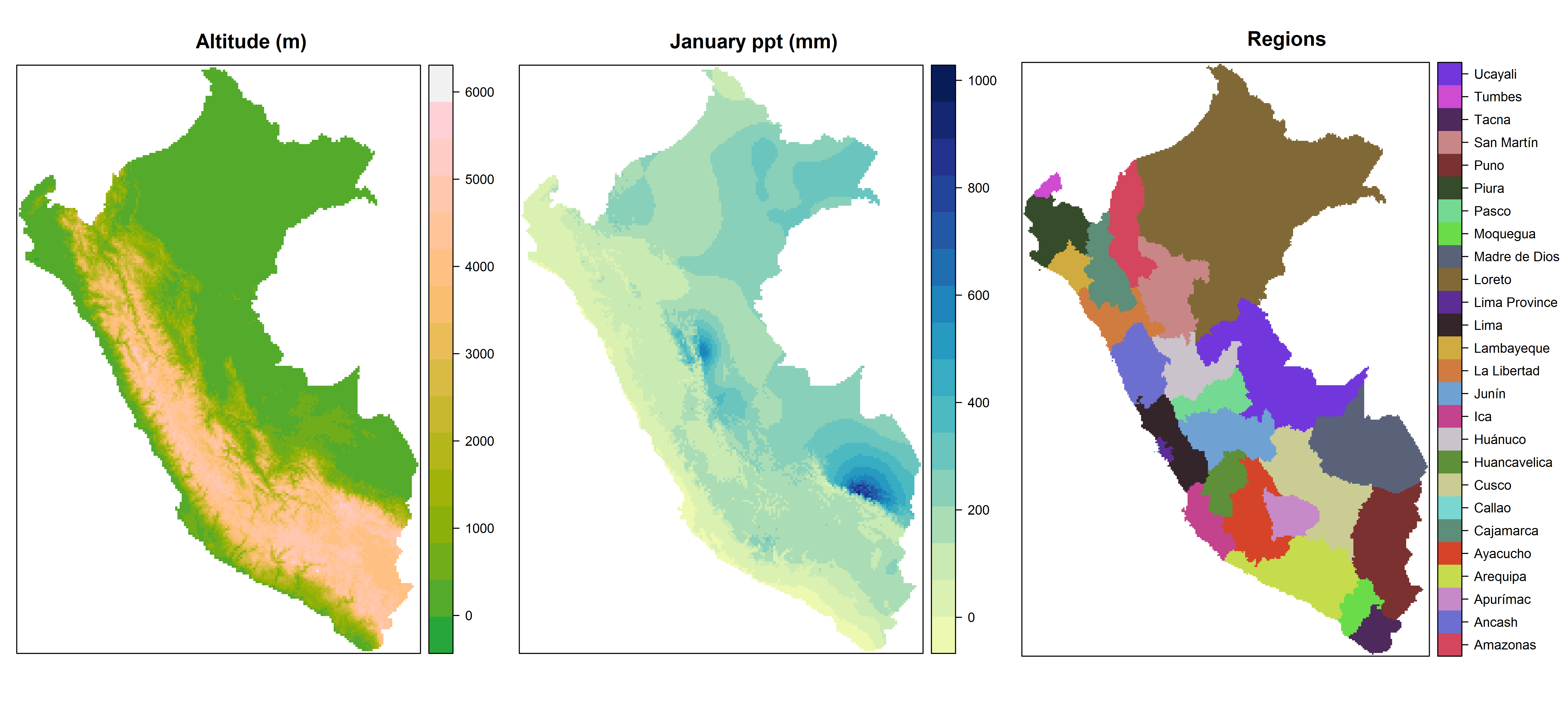
Let's compare the speed of **rasterDT** functions with their
**raster** package equivalents. To do so using realistic data, first
use `raster::getData()` to download and prepare three raster layers
which display the altitude, January precipitation, and political
regions of Peru at a resolution of one half arc minute.
(**PLEASE NOTE:** running the (fully reproducible) code below will
download several raster files into the working directory of your
current **R** session.)
``` r
library(rasterDT)
library(rasterVis)
library(microbenchmark)
## Altitude in m
altitude <- getData("alt", country = "PER", res = 0.5)
altitude <- crop(altitude, extent(altitude) - c(0, 0.2))
## Political subdivisions (categorical)
regions_shp <- getData("GADM", country = "PER", level = 1)
regions <- fasterizeDT(regions_shp, altitude, field = "NAME_1")
## January precipitation in mm
precip <- getData("worldclim", var = "prec", res = 0.5,
lon = -75, lat = -15)
precip1 <- crop(precip[[1]], regions)
precip1 <- mask(precip1, regions)
```
The three resulting rasters are displayed (using plotting calls not
shown here) in the figure below:
Next, to estimate the degree of speedup gained by using each
**rasterDT** function relative to its **raster** package equivalent,
we benchmark pairs of functions, executing equivalent calls 5 times
and comparing the average timings:
### `freqDT()` vs. `freq()`: ~6x speedup
``` r
microbenchmark(freqDT = freqDT(altitude),
freq = freq(altitude),
times = 5)
## Unit: milliseconds
## expr min lq mean median uq max neval cld
## freqDT 358.1587 373.9958 402.0715 375.5939 404.4736 498.1357 5 a
## freq 2481.5614 2570.1578 2583.9395 2605.2673 2611.1084 2651.6024 5 b
out_freqDT <- freqDT(altitude)
out_freq <- freq(altitude)
```
### `crosstabDT()` vs `crosstab()`: ~6x speedup
``` r
microbenchmark(crosstabDT = crosstabDT(altitude, regions),
crosstab = crosstab(altitude, regions),
times = 5)
## Unit: milliseconds
## expr min lq mean median uq max neval cld
## crosstabDT 934.0795 934.6892 1028.893 979.0466 1147.490 1149.160 5 a
## crosstab 6274.8551 6430.1598 6439.387 6454.1255 6509.927 6527.869 5 b
out_crosstabDT <- crosstabDT(altitude, regions)
out_crosstab <- crosstab(altitude, regions)
```
### `zonalDT()` vs `zonal()`: ~11x speedup
``` r
microbenchmark(zonalDT = zonalDT(altitude, regions, min),
zonal = zonal(altitude, regions, min),
times = 5)
## Unit: milliseconds
## expr min lq mean median uq max neval cld
## zonalDT 200.5657 204.6846 206.6882 207.9012 209.0513 211.2381 5 a
## zonal 2195.7178 2199.3366 2242.2448 2219.9958 2266.3005 2329.8735 5 b
out_zonalDT <- zonalDT(altitude, regions, min)
out_zonal <- zonal(altitude, regions, min)
```
### `subsDT()` vs `subs()`: ~23x speedup
``` r
dict <- zonalDT(altitude, regions, min, na.rm = TRUE)
microbenchmark(subsDT = subsDT(regions, dict),
subs = subs(regions, dict),
times = 5)
## Unit: milliseconds
## expr min lq mean median uq max neval cld
## subsDT 250.4851 254.4848 356.3356 259.0266 293.7392 723.9421 5 a
## subs 8077.3643 8086.8702 8167.4095 8184.9779 8186.2390 8301.5961 5 b
out_subsDT <- subsDT(regions, dict)
out_subs <- subs(regions, dict)
```
### `fasterizeDT()` vs `rasterize()`: ~25x speedup
``` r
## rasterize()'s field= argument can handle factor but not character vectors
regions_shp$NAME_FAC <- factor(regions_shp$NAME_1)
microbenchmark(fasterizeDT = fasterizeDT(regions_shp, altitude, field = "NAME_FAC"),
rasterize = rasterize(regions_shp, altitude, field = "NAME_FAC"),
times = 5)
## Unit: milliseconds
## expr min lq mean median uq max
## fasterizeDT 48.09048 49.00721 107.8917 51.78699 52.29528 338.2786
## rasterize 2693.34767 2734.66681 2748.1537 2763.89009 2771.21738 2777.6464
out_fasterizeDT <- fasterizeDT(regions_shp, altitude, field = "NAME_FAC")
out_rasterize <- rasterize(regions_shp, altitude, field = "NAME_FAC")
```