Data Science
Bayes and Validation
Alessandro D. Gagliardi
- Classification Problems
- Bayes Theorem
- Why we shouldn't use linear regression for classification problems
- Building Effective Classifiers
- Receiver Operating Characteristic (ROC) curves
- Naïve Bayes
- Lab
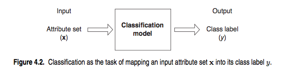
Classification Problems
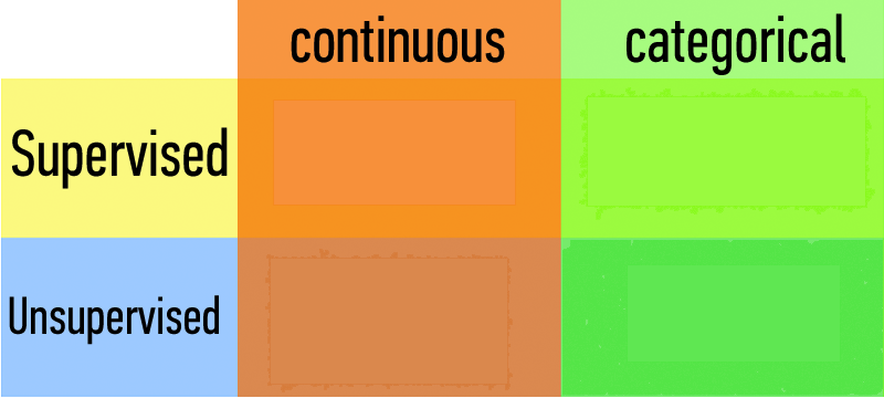
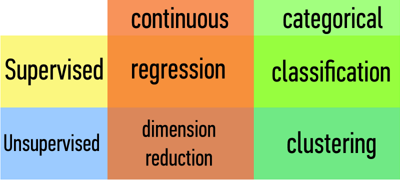
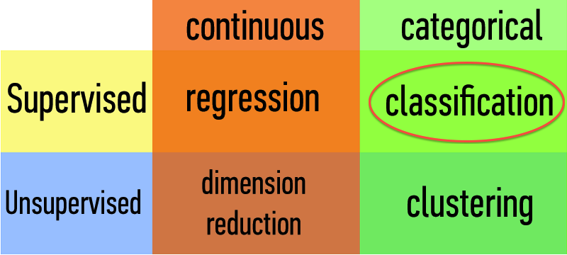
How does a classification problem work?
Input data, output predicted labels.
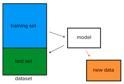
What steps does a classification problem require?
- Split the dataset
- Train the model
- Test the model
- Make predictions with new data
Model of breaking apart data for train, test, and output
Bayes Theorem
Problem
You have a database of 100 emails.
- 60 of those 100 emails are spam
- 48 of those 60 emails that are spam have the word "buy"
- 12 of those 60 emails that are spam don't have the word "buy"
- 40 of those 100 emails aren't spam
- 4 of those 40 emails that aren't spam have the word "buy"
- 36 of those 40 emails that aren't spam don't have the word "buy"
What is the probability that an email is spam if it has the word "buy"?
Solution
There are 48 emails that are spam and have the word "buy". And there are 52 emails that have the word "buy": 48 that are spam plus 4 that aren't spam. So the probability that an email is spam if it has the word "buy" is 48/52 = 0.92
If you understood this answer then you have understood the Bayes Theorem (in a nutshell)
Some Definitions:
Sample Space
Q. What do we call the space for all possible events?
A. This set is called the sample space $\Omega$.
(e.g. the numbers 1 through 6 on a six-sided die)
All events (such as $A$) are included in this space
The probability of the sample space $P(\Omega)$ is 1.
Intersecting Probabilities
Q. Consider two events $A$ & $B$. How can we characterize the intersection of these events?
A. With the joint probability of $A$ and $B$, written $P(AB)$.
e.g.
$P(A) =$ probability of being female
$P(B) =$ probability of having long hair
$P(AB)$ = the probability of being female & having long hair
Conditional Probability
Q. Suppose event $B$ has occurred. What quantity represents the probability of $A$ given this information about $B$?
A. The intersection of $A$ & $B$ divided by region $B$.
This is called the conditional probability of $A$ given $B$:
$$ P(A|B) = \frac{P(AB)}{P(B)} $$
Notice, with this we can also write $P(AB) = P(A|B) \times P(B)$.
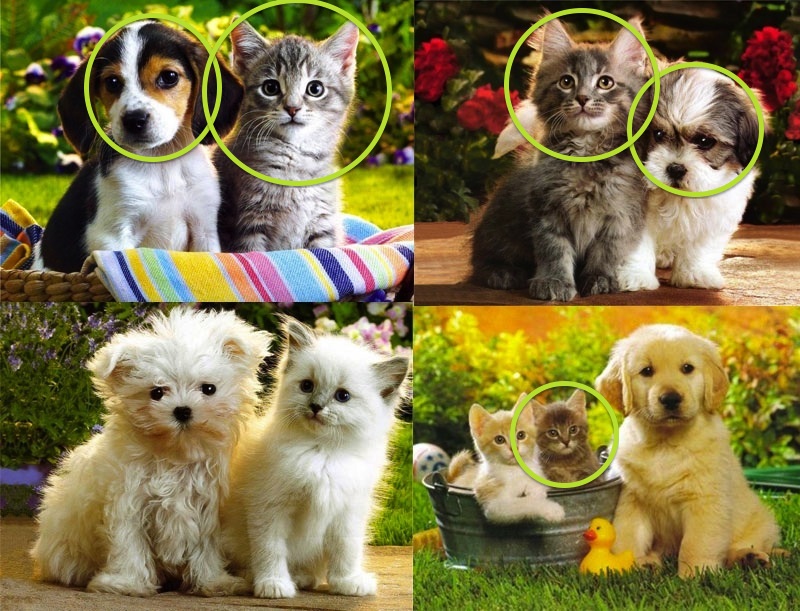
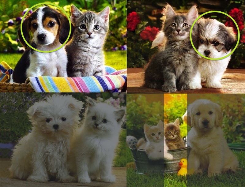
probability with the help of small animals
Sample Space

$P(puppy) = 4/9$
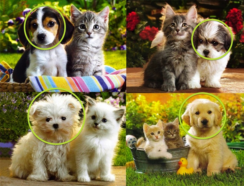
$P(dark) = 5/9$
$P(puppy|dark) = \frac{P(puppy, dark)}{P(dark)}$

$P(puppy|dark) = \frac{.444 \times .556}{.556} = \frac{.249}{.556} = .44$
Bayes Theorem
$P(AB) = P(A|B) \times P(B)\qquad$
$P(BA) = P(B|A) \times P(A)\qquad$ by substitution
But $P(AB) = P(BA)\qquad$ since event $AB =$ event $BA$
$\hookrightarrow P(A|B) \times P(B) = P(B|A) \times P(A)\>$ by combining the above
$\hookrightarrow P(A|B) = \frac{P(B|A) \times P(A)}{P(B)}\>$ by rearranging last step
Bayes’ Theorem
This result is called Bayes’ theorem. Here it is again:
$$ P(A|B) = \frac{P(B|A) \times P(A)}{P(B)} $$
Problem
this example taken from the Cartoon Guide to Statistics by Larry Gonick & Woollcott Smith
Suppose a rare disease infects one out of every 1000 people in a population...
and suppose that there is a good, but not perfect, test for this disease: if a person has the disease, the test comes back positive 99% of the time. One the other hand, the test also produces some false positives. About 2% of uninfected patients also test positive.
You just tested positive. Whate are your chances of having the disease?
Solution
We have two events to work with:
A : patient has the disease
B : patient tests positive
The information about the test's effectiveness can be written:
$$ P(A) = .001 $$ $$ P(B|A) = .99 $$ $$ P(B|\neg A) = .02 $$
$$ P(A|B) = ???$$
| A | not A | sum | |
|---|---|---|---|
| B | $P(A \& B)$ | $P(\neg A \& B)$ | $P(B)$ |
| not B | $P(A \&\neg B)$ | $P(\neg A \&\neg B)$ | $P(\neg B)$ |
| $P(A)$ | $P(\neg A)$ | $1$ |
$$ P(A \& B) = P(B|A)P(A) = (.99)(.001) = .00099 $$ $$ P(\neg A \& B) = P(B|\neg A)P(\neg A) = (.02)(.999) = .01998 $$
lets fill in some of these numbers:
| A | not A | sum | |
|---|---|---|---|
| B | $.00099$ | $.01998$ | $.02097$ |
| not B | $P(A \&\neg B)$ | $P(\neg A \&\neg B)$ | $P(\neg B)$ |
| $.001$ | $.999$ | $1$ |
arithmetic gives us the rest:
| A | not A | sum | |
|---|---|---|---|
| B | $.00099$ | $.01998$ | $.02097$ |
| not B | $.00001$ | $.97902$ | $.98903$ |
| $.001$ | $.999$ | $1$ |
From which we directly derive: $$ P(A|B) = \frac{P(A \& B)}{P(B)} = \frac{.00099}{.02097} = .0472 $$
Conditional Mean
The key variable in any regression problem is the conditional mean of the outcome variable y given the value of the covariate x:
Conditional mean: $E(y|x)$
In linear regression, we assume that this conditional mean is a linear function taking values in $(-\infty, +\infty)$:
$$ E(y|x) = \alpha + \beta x $$
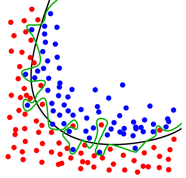
Why we shouldn't use linear regression for classification problems
Bounds can be greater than 0 and 1
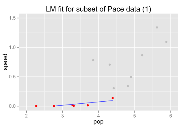
Sometimes extra data can really throw off our thresholds
Impossible to scale/predict when data throws off the regression
Example: the Whickham survey
Data on age, smoking, and mortality from a one-in-six survey of the electoral roll in Whickham, in the UK. The survey was conducted in 1972-1974 among women who were classified as current smokers or as never having smoked. A follow-up on those in the survey was conducted twenty years later.
%R print(head(Whickham))
Convert categories to binomial values:
%%R
Whickham$outcome <- as.integer(Whickham$outcome == 'Alive')
lm(outcome ~ 1, Whickham)
Modeling the intercept tells us that 71.9% of women surveyed were still alive 20-years later.
Modeling smoker
Add whether or not the woman was a smoker to the model:
%R print(lm(outcome ~ smoker, Whickham))
...smokers are 7.54% more likely to survive?!?
Modeling smoker + age
%R print(lm(outcome ~ smoker + age, Whickham))
A 20-year old smoker: $1.47 + 0.01 - 0.016 \times 20 = 1.16$
...has a $116\%$ chance of being a live 20-years later??
Probability(?) of Outcome
%%R -w 800 -h 600
ggplot(Whickham,aes(age,outcome,col=smoker))+geom_jitter(pos=position_jitter(h=.1))+geom_smooth(meth='lm')

Logistic Regression
In linear regression, we used a set of covariates to predict the value of a (continuous) outcome variable.
In logistic regression, we use a set of covariates to predict probabilities of (binary) class membership.
These probabilities are then mapped to class labels, thus solving the classification problem.
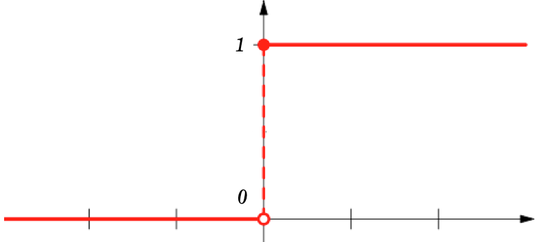
We use logistic regression to convert probabilities...
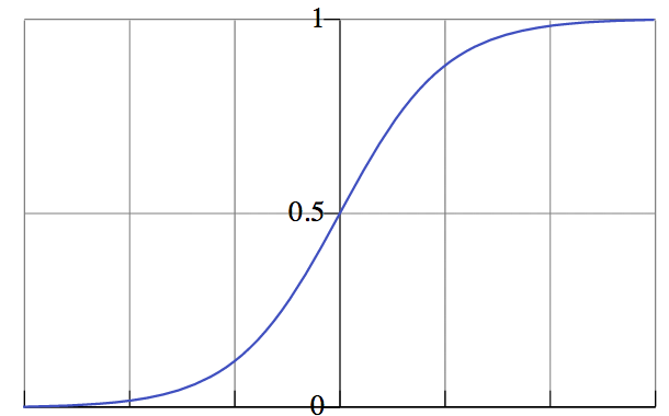
...into class labels!
Bernoulli (binomial) Distribution
%%R -w 800 -h 600
ggplot(Whickham, aes(age, outcome, color=smoker)) + geom_jitter(position = position_jitter(height = .1)) +
                    geom_smooth(method='glm', family='binomial') + xlab("Age") + ylab("Alive=1, Dead=0")

This utilizes logit for our link function.
Linear Regression Coefficients
Linear regression coefficients are fairly easy to interpret:
%R print(glm(outcome ~ smoker + age, family = "gaussian", data = Whickham)$coefficients)
$$ y = 1.47 + 0.01 \times (smoker = Yes) - 0.016 \times age $$
$y$ is the dependant variable
Logistic Regression Coefficients
Logistic regression coefficients are less straightforward:
%R print(glm(outcome ~ smoker + age, family = "binomial", data = Whickham)$coefficients)
$$ y = 7.599 - 0.205 \times (smoker = Yes) - 0.124 \times age $$
Take our 20-year old smoker:
$$ y = 7.6 - 0.2 - 0.123 \times 20 = 4.9 $$
But what does $y = 4.9$ mean?
Interepeting Results
In linear regression, the parameter $\beta$ represents the change in the response variable for a unit change in the covariate.
In logistic regression, $\beta$ represents the change in the logit function for a unit change in the covariate.
$$ \pi(1) = \frac{e^\beta}{1+e^\beta} $$
$$ \frac{e^{4.9}}{1+e^{4.9}} = 0.99 $$
In other words, our 20-year-old smoker has a 99% chance of surviving another 20 years.
Building Effective Classifiers
Where we find error
- Training error
- Generalization error
- Out of Sample (new data) error
Training error
What happens if we had no test data and only used a training set?
Q: Why should we use training & test sets?
Thought experiment:
Suppose instead, we train our model using the entire dataset
Q: How low can we push the training error?
- We can make the model arbitrarily complex (effectively “memorizing” the entire training set).
A: Down to zero!
This phenomenon is called overfitting.
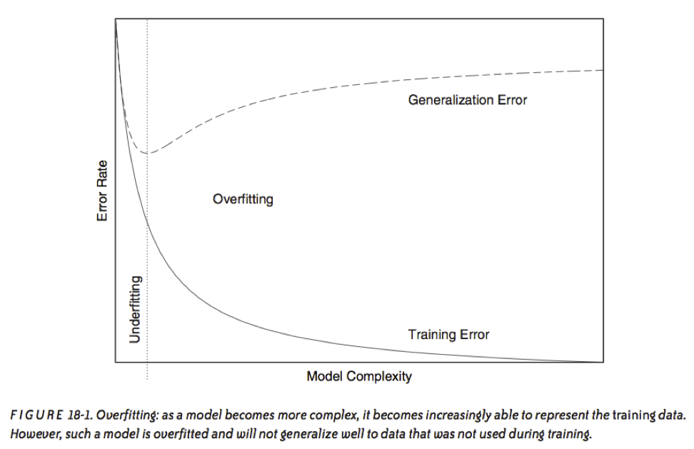 source: Data Analysis with Open Source Tools, by Philipp K. Janert. O’Reilly Media, 2011
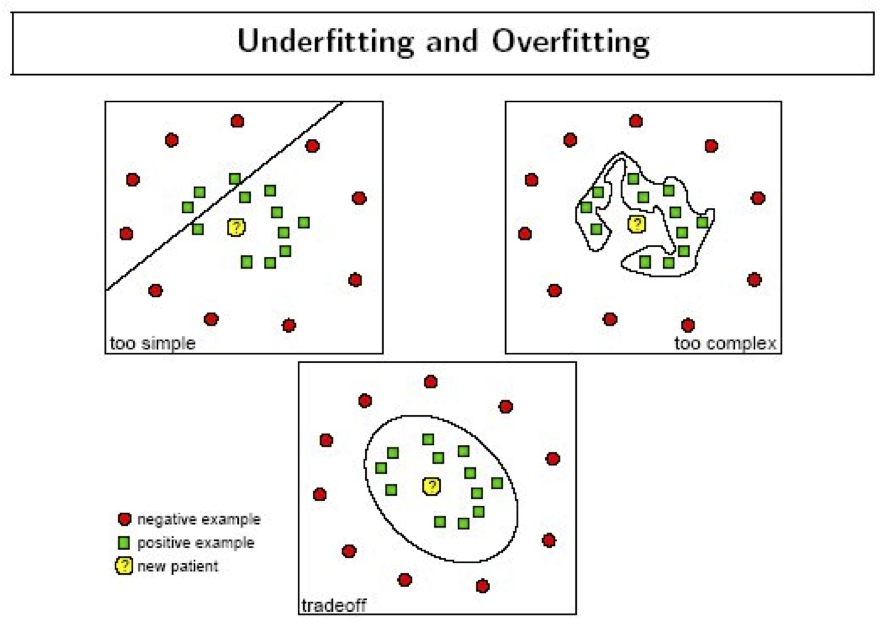
source: dtreg.com
source: dtreg.com
Q: Why should we use training & test sets?
Thought experiment:
Suppose instead, we train our model using the entire dataset.
Q: How low can we push the training error?
- We can make the model arbitrarily complex (effectively “memorizing” the entire training set). A: Down to zero!
A: Training error is not a good estimate of OOS accuracy.
Generalization Error
How well does the model generalize to unseen data?
Generalization Error
Try training the model on a subset of the data:
Does the error remain the same with different training data?
Generalization Error
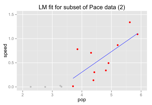
NO!
Generalization Error
- Generalization error gives a high variance estimate of OOS error
- Insufficient training can lead to incorrect model selection
Generalization Error
Something is still missing!
Q: How can we do better?
Thought experiment:
Different train/test splits will give us different generalization errors.
Q: What if we did a bunch of these?
A: Now you’re talking!
A: Cross-validation.
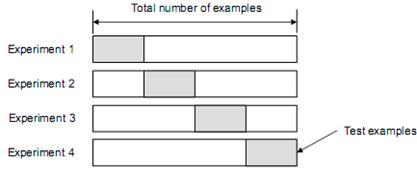
Cross Validation
Assessing a model using different subsets of the data for training and testing
Examples of Cross Validation
- N-fold cross validation
- Random sub-sampling validation
- Leave-one-out cross validation
N-fold cross validation
- Randomly split the dataset into n equal groups
- Use partition 1 as test set & union of other groups as training
- Find generalization error
- Repeat steps 2-3 using different group as test set at each iteration
- Take average generalization error as estimate of OOS accuracy
Features of n-fold cross-validation:
- More accurate estimate of OOS prediction error.
- More efficient use of data than single train/test split.
- Each record in our dataset is used for both training and testing.
- Presents tradeoff between efficiency and computational expense.
- 10-fold CV is 10x more expensive than a single train/test split
- Can be used for model selection.
Types of Errors
| Null hypothesis (H0) is true | Null hypothesis (H0) is false | |
|---|---|---|
| Reject null hypothesis | Type I error False positive |
Correct outcome True positive |
| Fail to reject null hypothesis | Correct outcome True negative |
Type II error False negative |
Notation for conditional probability
- Suppose that the patient has the disease (according to gold standard)
- Notation to specify the probability that the test for the patient is positive, given that the patient has the disease:
- P(Test positive | patient has disease)
- P(T+ | D+)
- This notation describes the conditional probability.
Sensitivity and Specificity
- We want the test to be positive when the patient has the disease:
- Sensitivity
- P(Test positive | patient has disease)
- We want the test to be negative when the patient does not have the disease:
- Specificity
- P(Test negative | patient does not have disease
High threshold:
Few false positive predictions, but lots of false negatives
- Good specificity = P(Test negative | patient does not have disease)
- Poor sensitivity = P(Test positive | patient has disease)
Low threshold:
Many false positive predictions, but few false negatives
- Poor specificity = P(Test negative | patient does not have disease)
- Good sensitivity = P(Test positive | patient has disease)
PPV and NPV
- Positive predictive value (PPV)
- P(patient has disease | Test positive )
- P(D+ | T+)
- Negative predictive value (NPV)
- P(patient does not have disease | Test negative )
- P(D- | T-)
ROC curves
- We plot sensitivity against 1 – specificity to create the ROC curve for a test
- For a single diagnostic test, sensitivity and specificity vary with the threshold we use.
- For a test that cannot separate the two classes, the ROC curve is a straight 45 degree line.
- Good tests approach the top left corner of the ROC curve.
- The area under the ROC curve (AUC) describes test accuracy
plt.figure(figsize=(12,8))
plt.plot(fpr, tpr, label='ROC curve (area = %0.2f)' % roc_auc)
plt.plot([0, 1], [0, 1], 'k--')
plt.xlabel('False Positive Rate'); plt.ylabel('True Positive Rate')
plt.legend(loc="lower right")

Naïve Bayes Classification
Bayesian Inference
Suppose we have a dataset with features $x_1, \ldots, x_n$ and a class label $C$.
What can we say about classification using Bayes’ theorem?
$$ P(C | x_1, \ldots, x_n) = \frac{P(x_1, \ldots, x_n | C) \times P(C)}{P(x_1, \ldots, x_n)} $$
Bayes’ theorem can help us to determine the probability of a record belonging to a class, given the data we observe.
Bayesian Inference
$$ P(C | x_1, \ldots, x_n) = \frac{P(x_1, \ldots, x_n | C) \times P(C)}{P(x_1, \ldots, x_n)} $$
In plain English the above equation can be written as
$$ \mbox{posterior} = \frac{\mbox{likelihood} \times \mbox{prior}}{\mbox{evidence}} $$
The Likelihood Function
$P(x_1, \ldots, x_n | C)$ is our likelihood function. It represents the joint probability of observing features $x_1, \ldots, x_n$ given that that record belongs to class $C$.
We can observe the value of the likelihood function from the training data.
The Prior
$P(C)$ is the prior probability of $C$. It represents the probability of a record belonging to class $C$ before the data is taken into account.
The value of the prior is also observed from the data.
The Normalization Constant
$P(x_1, \ldots, x_n)$ is the normalization constant. It doesn’t depend on $C$, and is generally ignored until the end of the computation.
The normalization constant doesn’t tell us much.
The Posterior
$P(C | x_1, \ldots, x_n)$ is the posterior probability of $C$. It represents the probability of a record belonging to class $C$ after the data is taken into account.
The goal of any Bayesian computation is to find ("learn") the posterior distribution of a particular variable.
Bayesian Inference
The idea of Bayesian inference, then, is to update our beliefs about the distribution of $C$ using the data ("evidence") at our disposal.
$$ P(C | x_1, \ldots, x_n) = \frac{P(x_1, \ldots, x_n | C) \times P(C)}{P(x_1, \ldots, x_n)} $$
Then we can use the posterior for prediction.
Naïve Bayesian Classification
Q. What piece of the puzzle we’ve seen so far looks like it could intractably difficult in practice?
Naïve Bayesian Classification
Remember the likelihood function?
$P(x_1, \ldots, x_n | C)$
Observing this exactly would require us to have enough data for every possible combination of features to make a reasonable estimate.
Naïve Bayesian Classification
Q. What piece of the puzzle we’ve seen so far looks like it could intractably difficult in practice?
A. Estimating the full likelihood function.
Naïve Bayesian Classification
Q. So what can we do about it?
A. Make a simplifying assumption. In particular, we assume that the features $x_1, \ldots, x_n$ are conditionally independent from each other:
$$ P(x_1, \ldots, x_n | C) \approx P(x_1 | C) \times P(x_2 | C) \times \ldots \times P(x_n|C) $$
This "naïve" assumption simplifies the likelihood function to make it tractable.
LAB
In the DAT6 folder, from the command line:
git commit -am ...
git checkout gh-pages
git pull
git checkout personal
git merge gh-pages
ipython notebook
Then open DS_Lab09-TM