
PerfView is a tool for quickly and easily collecting and viewing both time and memory performance data. PerfView uses the Event Tracing for Windows (ETW) feature of the operating system which can collect information machine wide a variety of useful events as described in the advanced collection section. ETW is the same powerful technology the windows performance group uses almost exclusively to track and understand the performance of windows, and the basis for their Xperf tool. PerfView can be thought of a simplified and user friendly version of that tool. In addition PerfView has ability to collect .NET GC Heap information for doing memory investigation (Even for very large GC heaps). PerfView's ability to decode .NET symbolic information as well as the GC heap make PerfView ideal for managed code investigations .
Deploying and Using PerfView
PerfView was designed to be easy to deploy and use. To deploy PerfView simply copy the PerfView.exe to the computer you wish to use it on. No additional files or installation step is needed. PerfView features are 'self-discoverable'. The initial display is a 'quick start' guide that leads you through collecting and viewing your first set of profile data. There is also a built in tutorial. Hovering the mouse over most GUI controls will give you short explanations, and hyperlinks send you to the most appropriate part of this user's guide. Finally PerfView is 'right click enabled' which means that you want to manipulate data in some way, right clicking allows you to discover what PerfView's can do for you.
PerfView is a V4.6.2 .NET application. Thus you need to have installed a V4.6.2 .NET Runtime on the machine which you actually run PerfView. On Windows 10 and Windows Server 2016 has .NET V4.6.2. On other supported OS you can install .NET 4.6.2 from standalone installer. PerfView is not supported on Win2K3 or WinXP. While PerfView itself needs a V4.6.2 runtime, it can collect data on processes that use V2.0 and v4.0 runtimes. On machines that don't have V4.6.2 or later of the .NET runtime installed, it is also possible to collect ETL data with another tool (e.g. XPERF or PerfMonitor) and then copy data file to a machine with V4.6.2 and view it with PerfView.
PerfView was designed to collect and analyze both time and memory scenarios.
See also PerfView Reference Guide.
Hopefully the documentation does a reasonably good job of answering your most common questions about PerfView and performance investigation in general. If you have a question, you should certainly start by searching the user's guide for information
Inevitably however, there will be questions that the docs don't answer, or features you would like to have that don't yet exist, or bugs you want to report. PerfView is an GitHub open source project and you should log questions, bugs or other feedback at
If you are just asking a question there is a Label called 'Question' that you can use to indicate that. If it is a bug, it REALLY helps if you supply enough information to reproduce the bug. Typically this includes the data file you are operating on. You can drag small files into the issue itself, however more likely you will need to put the data file in the cloud somewhere and refer to it in the issue. Finally if you are making a suggestion, the more specific you can be the better. Large features are much less likely to ever be implemented unless you yourself help with the implementation. Please keep that in mind.
You can get the latest version of PerfView by going to the PerfView GitHub Download Page
See Also Tutorial of a GC Heap Memory Investigation
Perhaps the best way to get started is to simply try out the tutorial example. On windows 7 it is recommended that you doc your help as described in help tips. PerfView comes with two tutorial examples 'built in'. Also we strongly suggest that any application you write have performance plan as described in part1 and part2 of Measure Early and Often for Performance .
To run the 'Tutorial' example:
You can also run the tutorial example by typing 'PerfView run tutorial' at the command line. See collecting data from the command line for more.
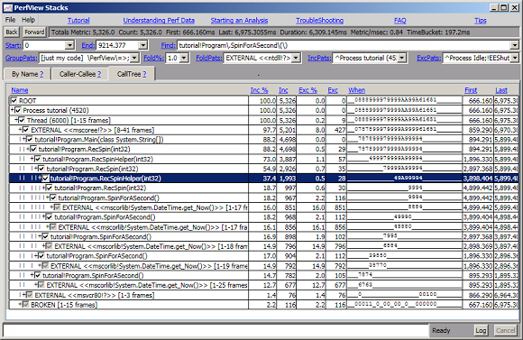
After selecting 'Tutorial.exe' as the process of interest, PerfView brings up the stack viewer looking something like this:
This view shows you where CPU time was spent. PerfView took a sample of where each processor is (including the full stack), every millisecond (see understanding perf data) and the stack viewer shows these samples. Because we told PerfView we were only interested in the Tutorial.exe process this view has been restricted (by 'IncPats') to only show you samples that were spent in that process.
It is always best to begin your investigation by looking at the summary information at the top of the view. This allows you to confirm that indeed the bulk of your performance problem is related to CPU usage before you go chasing down exactly where CPU is spent. This is what the summary statistics are for. We see that the process spent 84% of its wall clock time consuming CPU, which merits further investigation. Next we simply look at the 'When' column for the 'Main' method in the program. This column shows how CPU was used for that method (or any method it calls) over the collection time interval. Time is broken into 32 'TimeBuckets' (in this case we see from the summary statistics that each bucket was 197 msec long), and a number or letter represents what % of 1 CPU is used. 9s and As mean you are close to 100% and we can see that over the lifetime of the main method we are close to 100% utilization of 1 CPU most of the time. Areas outside the main program are probably not interesting to use (they deal with runtime startup and the times before and after process launch), so we probably want to 'zoom in' to that area.
It is pretty common that you are only interested in part of the trace. For example you may only care about startup time, or the time from when a mouse was clicked and when the menu was displayed. Thus zooming in is typically one of first operations you will want to do. zooming in is really just selecting a region of time for investigation. The region of time is displayed in the 'start' and 'end' textboxes. These can be set in three ways
Try out each of these techniques. For example to 'zoom into' just the main method, simply drag the mouse over the 'First' and 'Last' times to select both, right click, and Select Time Range. You can hit the 'Back' button to undo any changes you made so you can re-select. Also notice that each text box remembers the last several values of that box, so you can also 'go back' particular past values by selecting drop down (small down array to the right of the box), and selecting the desired value.
For GUI applications, it is not uncommon to take a trace of the whole run but then 'zoom into' points where the users triggered activity. You can do this by switching to the 'CallTree' tab. This will show you CPU starting from the process itself. The first line of is the View is 'Process32 tutorial.exe' and is a summary of the CPU time for the entire process. The 'when' column shows you CPU for the process over time (32 time buckets). In a GUI application there will be lulls where no CPU was used, followed by bursts of higher CPU use corresponding to user actions. These show up in the numbers in the 'when' column. By clicking on a cell in the 'when' column, selecting a range, right clicking and selecting SetTimeRange (or Alt-R), you can zoom into one of these 'hot spots' (you may have to zoom in more than once). Now you have focused in on what you are interested in (you can confirm by looking at the methods that are called during that time). This is a very useful technique.
For managed applications, you will always want to zoom into the main method before starting your investigation. The reason is that when profile data is collected, after Main has exited, the runtime spends some time dumping symbolic information to the ETW log. This is almost never interesting, and you want to ignore it in your investigation. Zooming into the Main method will do this.
Right clicking, and select 'Lookup Symbols'. After looking up the symbols it will become
If you are doing an unmanaged investigation there are probably a handful of DLLs you will need symbols for. A common workflow is to look at the byname view and while holding down the CTRL key select all the cells that contain dlls with large CPU time but unresolved symbols. Then right click -> Lookup Symbols, and PerfView will look them all up in bulk. See symbol resolution for more details or if lookup symbols fails.
PerfView starts you with the 'ByName view' for doing a bottom-up analysis (see also starting an analysis). In this view you see every method that was involved in a sample (either a sample occurred in the method or the method called a routine that had a sample). Samples can either be exclusive (occurred in within that method), or inclusive (occurred in that method or any method that method called). By default the by name view sorts methods based on their exclusive time (see also Column Sorting). This shows you the 'hottest' methods in your program.
Typically the problem with a 'bottom-up' approach is that the 'hot' methods in your program are
In both cases, you don't want to see these helper routines, but rather the lowest 'semantically interesting' routine. This is where PerfView's powerful grouping features comes into play. By default PerfView groups samples by
For example, the top line in the ByName view is
This is an example of an 'entry group'. 'OTHER' is the group's name and mscorlib!System.DateTime.get_Now() is the method that was called that entered the group. From that point on any methods that get_Now() calls that are within that group are not shown, but rather their time is simply accumulated into this node. Effectively this grouping says 'I don't want to see the internal workings of functions that are not my code, but I do want see public methods I used to call that code. To give you an idea of how useful this feature is, simply turn it off (by clearing the value in the 'GroupPats' box), and view the data. You will see many more methods with names of internal functions used by 'get_Now' which just make your analysis more difficult. (You can use the 'back' button to quickly restore the previous group pattern).
The other feature that helps 'clean up' the bottom-up view is the Fold % feature. This feature will cause all 'small' call tree nodes (less than the given %) to be automatically folded into their parent. Again you can see how much this feature helps by clearing the textbox (which means no folding). With that feature off, you will see many more entries that have 'small' amounts of time. These small entries again tend to just add 'clutter' and make investigation harder.
A quick way of accomplishing (2) is to add the pattern '!?' . This pattern says to fold away any nodes that don't have a method name. See foldPats textbox for more. This leaves us with very 'clean' function view that has only semantically relevant nodes in it.
Review: what all this time selection, grouping and folding is for?
The first phase of a perf investigation is forming a 'perf model' The goal is it assign times to SEMANTICALLY RELEVANT nodes (things the programmer understands and can do something about). We do that by either forming a semantically interesting group and assigning nodes to it, or by folding the node into an existing semantically relevant group or (most commonly) leveraging entry points into large groups (modules and classes), as handy 'pre made' semantically relevant nodes. The goal is to group costs into a relatively small number (< 10) of SEMANTICALLY RELEVANT entries. This allows you to reason about whether that cost is appropriate or not, (which is the second phase of the investigation).
One of the nodes that is left is a node called 'BROKEN'. This is a special node that represents samples whose stack traces were determined to be incomplete and therefore cannot be attributed properly. As long as this number is small (< a few %) then it can simply be ignored. See broken stacks for more.
PerfView displays both the inclusive and exclusive time as both a metric (msec) as well as a % because both are useful. The percentage gives you a good idea of the relative cost of the node, however the absolute value is useful because it very clearly represents 'clock time' (e.g. 300 samples represent 300 msec of CPU time). The absolute value is also useful because when the value gets significantly less than 10 it becomes unreliable (when you have only a handful of samples they might have happened 'by pure chance' and thus should not be relied upon.
The bottom up view did an excellent job of determining that the get_Now() method as well as the 'SpinForASecond' consume the largest amount of time and thus are worth looking at closely. This corresponds to our expectations given the source code in Tutorial.cs. However it can also be useful to understand where CPU time was consumed from the top down. This is what the CallTree view is for. Simply by clicking the 'CallTree' tab of the stack viewer will bring you to that view. Initially the display only shows the root node, but you can open the node by clicking on the check box (or hitting the space bar). This will expand the node. As long as a node only has one child, the child node is also auto-expanded, to save some clicking. You can also right click and select 'expand-all' to expand all nodes under the selected node. Doing this on the root node yields the following display
Notice how clean the call tree view is, without a lot of 'noise' entries. In fact this view does a really good job of describing what is going on. Notice it clearly shows the fact that Main calls 'RecSpin, which runs for 5 seconds (from 894ms to 5899msec) consuming 4698 msec of CPU while doing so (The CPU is not 5000msec because of the overheads of actually collecting the profile (and other OS overhead which is not attributed to this process as well as broken stacks), which typically run in the 5-10% range. In this case it seems to be about 6%). The 'When' column also clearly shows how one instance of RecSpin runs SpinForASecond (for exactly a second) and then calls a RecSpinHelper which consumes close to 100% of the CPU for the rest of the time. . The call Tree is a wonderful top-down synopsis.
All of the filtering and grouping parameters at the top of the view affect any of the view (byname, caller-callee or CallTree), equally. We can use this fact and the 'Fold %' functionality to get an even coarser view of the 'top' of the call tree. With all nodes expanded, simply right click on the window and select 'Increase Fold %' (or easier hit the F7 key). This increases the number in the Fold % textbox by 1.6X. By hitting the F7 key repeatedly you keep trimming down the 'bottoms' of the stacks until you only see methods that use a large amount of CPU time. The following image shows the CallTreeView after hitting F7 seven times.
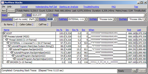
You can restore the previous view by either using the 'Back' button, the Shift-F7 key (which decreases the Fold%) or by simply selecting 1 in the Fold% box (e.g. from the drop down menu).
Getting a course view of the tree is useful but sometimes you just want to restrict your attention to what is happening at a single node. For example, if the inclusive time for BROKEN stacks is large, you might want to view the nodes under 'BROKEN' stacks to get an idea what samples are 'missing' from their proper position in the call tree. you can do this easily by viewing the BROKEN node in the Caller-callee view. To do this right click on the BROKEN node, and select Goto -> Caller-callee (or type Alt-C). Because so few samples are in our trace are BROKEN this node is not very interesting. By setting Fold % to 0 (blank) you get the following view
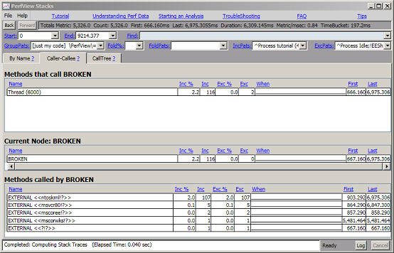
The view is broken in to three grids. The middle piece shows the 'current node', in this case 'BROKEN'. The top grid shows all nodes that call into this focus node. In the case of BROKEN nodes are only on one thread. The bottom graph shows all nodes that are called by 'BROKEN' sorted by inclusive time. We can see that most of the broken nodes came from stacks that originated in the 'ntoskrnl' dll (this is the Windows OS Kernel) To dig in more we would first need to resolve symbols for this DLL. See symbol resolution for more.
While groups are a very powerful feature for understanding the performance of your program at a 'coarse' level, inevitably, you wish to 'Drill into' those groups and understand the details of PARTICULAR nodes in detail. For example, If we were a developer responsible for the DateTime.get_Now(), we would not be interested in the fact that it was called from 'SpinForASecond' routine but what was going on inside. Moreover we DON'T want to see samples from other parts of the program 'cluttering' the analysis of get_Now(). This is what the 'Drill Into' command is for. If we go back to the 'ByName' view and select the 3792 samples 'Inc' column of the 'get_Now' right click, and select 'Drill Into', it brings a new window where ONLY THOSE 3792 samples have been extracted.
Initially Drilling in does not change any filter/grouping parameters. However, now that we have isolated the samples of interest, we are free to change the grouping and folding to understand the data at a new level of abstraction. Typically this means ungrouping something. In this case we would like to see the detail of how mscorlib!get_Now() works, so we want to see details inside mscorlib. To do this we select the 'mscorlib!DateTime.get_Now() node, right click, and select 'Ungroup Module'. This indicates that we wish to ungroup any methods that were in the 'mscorlib' module. This allows you to see the 'inner structure' of that routine (without ungrouping completely) The result is the following display

At this point we can see that most of the 'get_Now' time is spend in a function called 'GetUtcOffsetFromUniversalTime' and 'GetDatePart' We have the full power of the stack viewer at our disposal, folding, grouping, using CallTree or caller-callee views to further refine our analysis. Because the 'Drill Into' window is separate from its parent, you can treat is as 'disposable' and simply discard it when you are finished looking at this aspect of your program's performance.
In the example above we drilled into the inclusive samples of method. However you can also do the same thing to drill into exclusive samples. This is useful when user callbacks or virtual functions are involved. Take for example a 'sort' routine that has internal helper functions. In that case it can be useful to segregate those samples that were part of the nodes 'internal helpers' (which would be folded up as exclusive samples of 'sort') from those that were caused by the user 'compare' function (which would typically not be grouped as exclusive samples because it crossed a module boundary). By drilling into the exclusive samples of 'sort' and then ungrouping, you get to see just those samples in 'sort' that were NOT part of the user callback. Typically this is EXACTLY what the programmer responsible for the 'sort' routine would want to see.
Once the analysis has determined methods are potentially inefficient, the next step is to understand the code enough to make an improvement. PerfView helps with this by implementing the 'Goto Source' functionality. Simply select a cell with a method name in it, right click and choose Goto Source (or use Alt-D (D for definition)). PerfView with then attempt to look up the source code and if successful will launch a text editor window. For example, if you select the 'SpinForASecond' cell in the ByName view and select Goto Source the following window is displayed.

As you can see, the particular method is displayed and each line has been prefixed with the cost (in this case CPU MSec) spent on that line. in this view it shows 4.9 seconds of CPU time were spent on the first line of the method.
Unfortunately, prior to V4.5 of the .NET Runtime, the runtime did not emit enough information into the ETL file to resolve a sample down to a line number (only to a method). As a result while PerfView can bring up the source code, it can't accurately place samples on particular lines unless the code was running on V4.5 or later. When PerfView does not have the information it needs it simply attributes all the cost to the first line of the method. This is in fact what you see in the example above. If you run your example on a V4.5 runtime, you would get a more interesting distribution of cost. This problem does not exist for native code (you will get line level resolution). Even on old runtime versions, however, you at least have an easy way to navigate to the relevant source.
PerfView finds the source code by looking up information in the PDB file associated with the code. Thus the first step is that PerfView must be able to find the PDB file. By default most tools will place the complete path of the PDB file inside the EXE or DLL it builds, which means that if you have not moved the PDB file (and are on the machine you built on), then PerfView will find the PDB. It then looks in the PDB file which contain the full path name of each of the source files and again, if you are on the machine that built the binary then PerfView will find the source. So if you run on the same machine you build on, it 'just works'.
However it is common to not run on the machine you built on, in which case PerfView needs help. PerfView follows the standard conventions for other tools for locating source code. In particular if the _NT_SYMBOL_PATH variable is set to a semicolon separated list of paths, it will look in those places for the PDB file. In addition if _NT_SOURCE_PATH is set to a semicolon separated list of paths, it will search for the source file in subdirectories of each of the paths. Thus setting these environment variables will allow PerfView's source code feature to work on 'foreign' machines. You can also set the _NT_SYMBOL_PATH and _NT_SOURCE_PATH inside the GUI by using the menu items on the File menu on the stack viewer menu bar.
See Also Tutorial of a Time-Based Investigation. While there currently is no tutorial on doing a GC heap analysis, if you have not walked the time based investigation tutorial you should do so. Many of the same concepts are used in a memory investigation. You should also take a look at
TUTORIAL NOT COMPLETE
As mentioned in the introduction, ETW is light weight logging mechanism built into the Windows Operating system that can collect a broad variety of information about what is going on in the machine. There are two ways PerfView supports for collecting ETW profile data.
You can also automate the collection of profile data by using command line options. See collecting data from the command line for more.
If you intend to do a wall clock time investigation
By default PerfView chooses a set of events that does not generate too much data but is useful for a variety of investigations. However wall clock investigations require events that are too voluminous to collect by default. Thus if you wish to do a wall clock investigation, you need to set the 'Thread Time' checkbox in the collection dialog.
If you intend to copy the ETL file to another machine for analysis
By default to save time PerfView does NOT prepare the ETL file so that it can be analyzed on a different machine (see merging). Moreover, there is symbolic information (PDBS for NGEN images), that also needs to be included if the data is to work well on any machine). If you are intending to do this you need to merge and include the NGEN pdbs by using the 'ZIP' command. You can do this either by
Once the data has been zipped not only does the file contain all the information needed to resolve symbolic information, but it also has been compressed for faster file copies. If you intend to use the data on another machine, please specify the ZIP option.
The result of collecting data is an ETL file (and possibly a .kernel.ETL file as discussed in merging). When you double click on the file in the main viewer it opens up 'children views' of the data that was collected. One of these items will be the 'CPU Stacks' view. Double clicking on that will bring up a stack viewer to view the samples collected. The data in the ETL file contains CPU information for ALL processes in the system, however most analyses concentrate on a single process. Because of this before the stack viewer is displayed a dialog box to select a process of interest is displayed first.
By default, this dialog box contains a list of all processes that were active at the time the trace was collected sorted by the amount of CPU time each process consumed. If you are doing a CPU investigation, there is a good chance the process of interest is near the top of this list. Simply double clicking on the desired process will bring up the stack viewer filtered to the process you chose.
The process view can be sorted by any of the columns by clicking on the column header. Thus if you wish to find the process that was started most recently you can sort by start time to find it quickly. If the view is sorted by name, if you type the first character of the process name it will navigate to the first process with that name.
Process Filter Textbox The box just above the list of processes. If you type text in this box, then only processes that match this string (PID, process name or command line, case insensitive) will be displayed. The * character is a wild card. This is a quick way of finding a particular process.
If you wish to see samples for more than one process for your analysis click the 'All Procs' button.
Note that the ONLY effect of the process selection dialog box is to add an 'Inc Pats' filter that matches the process you chose. Thus the dialog box is really just a 'friendly interface' to the more powerful filtering options of the stack viewer. In particular, the stack viewer still has access to all the samples (even those outside the process you selected), it is just that it filters it out because of the include pattern that was set by the dialog box. This means that you can remove or modify this filter at a later point in the analysis.
The data shown by default in the PerfView stack viewer are stack traces taken every millisecond on each processor on the system. Every millisecond, whatever process is running is stopped and the operating system 'walks the stack' associated with the running code. What is preserved when taking a stack trace is the return address of every method on the stack. Stackwalking may not be perfect. It is possible that the OS can't find the next frame (leading to broken stacks) or that an optimizing compiler has removed a method call (see missing frames), which can make analysis more difficult. However for the most part the scheme works well, and has low overhead (typically 10% slowdown), so monitoring can be done on 'production' systems.
On lightly loaded system, many CPUs are typically in the 'Idle' process that the OS run when there is nothing else to do. These samples are discarded by PerfView because they are almost never interesting. All other samples are kept however, regardless of what process they were taken from. Most analyses focus on a single process, and further filter all samples that did not occur in the process of interest, however PerfView also allows you to also look at samples from all processes as one large tree. This is useful in scenarios where more than one process is involved end-to-end, or when you need to run an application several times to collect enough samples.
Because the samples are taken every millisecond per processor, each sample represents 1 millisecond of CPU time. However exactly where the sample is taken is effectively 'random', and so it is really 'unfair' to 'charge' the full millisecond to the routine that happened to be running at the time the sample was taken. While this is true, it is also true that as more samples are taken this 'unfairness' decreases as the square root of the number of samples. If a method has just 1 or 2 samples it could be just random chance that it happened in that particular method, but methods with 10 samples are likely to have truly used between 7 and 13 samples (30% error). Routines with 100 samples are likely to be within 90 and 110 (10% error). For 'typical' analysis this means you want at least 1000 and preferably more like 5000 samples (There are diminishing returns after 10K). By collecting a few thousand samples you ensure that even moderately 'warm' methods will have at least 10 samples, and 'hot' methods will have at least 100s, which keep the error acceptably small. Because PerfView does not allow you to vary the sampling frequency, this means that you need to run the scenario for at least several seconds (for CPU bound tasks), and 10-20 seconds for less CPU bound activities.
If the program you wish to measure cannot easily be changed to loop for the required amount of time, you can create a batch file that repeatedly launches the program and use that to collect data. In this case you will want to view the CPU samples for all processes, and then use a GroupPat that erases the process ID (e.g. process {%}=>$1) and thus groups all processes of the same name together.
Even with 1000s of samples, there is still 'noise' that is at least in the 3% range (sqrt(1000) ~= 30 = 3%). This error gets larger as the methods / groups being investigated have fewer samples. This makes it problematic to use sample based profiling to compare two traces to track down small regressions (say 3%). Noise is likely to be at least as large as the 'signal' (diff) you are trying to track down. Increasing the number of samples will help, however you should always keep in mind the sampling error when comparing small differences between two traces.
Because a stack trace is collected for each sample, every node has both an exclusive metric (the number of samples that were collected in that particular method) and an inclusive metric (the number of samples that collected in that method or any method that method called). Typically you are interested in inclusive time, however it is important to realize that folding (see FoldPats and Fold %) and grouping artificially increase exclusive time (it is the time in that method (group) and anything folded into that group). When you wish to see the internals of what was folded into a node, you Drill Into the groups to open a view where the grouping or folding can be undone.
If you have not done so, consider walking through the tutorial and best practices from Measure Early and Often for Performance .
The default stack viewer in PerfView analyzes CPU usage of your process. There are three things that you should always do immediately when starting a CPU analysis of a particular process.
If either of the above conditions fail, the rest of your analysis will very likely be inaccurate. If you don't have enough samples you need to go back and recollect so that you get more, modifying the program to run longer, or running the program many times to accumulate more samples. If you program is running for long enough (typically 5-20 seconds), and you still don't have at least 1000 samples, it is likely it is because CPU is NOT the bottleneck. It is very common in STARTUP scenarios that CPU is NOT the problem but that the time is being spent fetching data from the disk. It is also possible that the program is waiting on network I/O (server responses) or responses from other processes on the local system. In all of these cases the time being wasted is NOT governed by how much CPU time is used, and thus a CPU analysis is inappropriate.
You can quickly determine if your process is CPU bound by looking at the 'When' column for your 'top most' method. If the When column has lots of 9s or As in it over the time it is active then it is likely the process was CPU bound during that time. This is the time you can hope to optimize and if it is not a large fraction of the total time of your app, then optimizing it will have little overall effect (See Amdahl's Law). Switching to the CallTree view and looking at the 'When' column of some of the top-most methods in the program is a good way of confirming that your application is actually CPU bound..
Finally you may have enough samples, but you lack the symbolic information to make sense of them. This will manifest with names with ? in them. By default .NET code should 'just work'. For unmanaged code you need to tell PerfView which DLLs you are interested in getting symbols for. See symbol resolution for more. You should also quickly check that you don't have many broken stacks as this too will interfere with analysis.
Once you have determined that CPU is actually important to optimize you have a choice of how to do your analysis. Performance investigations can either be 'top-down' (starting with the Main program and how the time spent there is divided into methods it calls), or 'bottom-up' (starting with methods at 'leaf' methods where samples were actually taken, and look for methods that used a lot of time). Both techniques are useful, however 'bottom-up' is usually a better way to start because methods at the bottom tend to be simpler and thus easier to understand and have intuition about how much CPU they should be using.
PerfView starts you out in the 'ByName' view that is appropriate starting point for a bottom-up analysis. It is particularly important in a bottom up analysis to group methods into semantically relevant groupings. By default PerfView picks a good set starting group (called 'just my code'). In this grouping any method in any module that lives in a directory OTHER than the directory where the EXE lives, is considered 'OTHER' and the entry group feature is used group them by the method used to call out to this external code. See the tutorial more on the meaning of 'Just My Code' grouping, and the GroupPats reference for more on grouping.
For simple applications the default grouping works well. There are other predefined groupings in the dropdown of the GroupPats box, and you are free to create or extend these as you need. You know that you have a 'good' set of groupings when what you see in the 'ByName' view are method names that are semantically relevant (you recognize the names, and know what their semantic purpose is), there are not too many of them (less than 20 or so that have an interesting amount of exclusive time), but enough that break the program into 'interesting' pieces that you can focus on in turn (by Drilling Into).
One very simple way of doing this is to increase the Fold % , which folds away small nodes. There is a shortcuts that increase (F7 key) or decrease (Shift F7) this by 1.6X. Thus by repeatedly hitting F7, you can 'clump' small nodes into large nodes until only a few survive and are displayed. While this is fast and easy, it does not pay attention to how semantically relevant the resulting groups are. As a result it may group things in poor ways (folding away small nodes that were semantically relevant, and grouping them into 'helper routines' that you don't much want to see). Nevertheless, it is so fast and easy it is always worth at least trying to see what happens. Moreover it is almost always valuable to fold away truly small nodes. Even if a node is semantically relevant, if it uses < 1% of the total CPU time, you probably don't care about it.
Typically the best results occur when you use Fold % in the 1-10% range (to get rid of the smallest nodes), and then selectively fold way any semantically uninteresting nodes that are left. This can be done easily looking at the 'ByName' view, holding the 'Shift' key down, and selecting every node on the graph that has some exclusive time (they will be toward the top), and you DON'T recognize. After you have completed your scan, simply right click and select 'Fold Item' and these node will be folded into their caller disappearing from the view. Repeat this until there are no nodes in the display that use exclusive time that are semantically irrelevant. What you have left is what you are looking for.
During the first phase of an investigation you spend your time forming semantically relevant groups so you can understand the 'bigger picture' of how the time spent in hundreds of individual methods can be assigned a 'meaning'. Typically the next phase is to 'Drill into' one of these groups that seems to be using too much time. In this phase you are selectively ungrouping a semantic group to understand what is happening at the next 'lower level' of abstraction.
You accomplish this with two commands
Typically if 'Ungroup' or 'Ungroup Module command does not work well, use 'Clear all Folding' If that does not work well, clear the 'GroupPats' textbox which will show you the most 'ungrouped' view. if this view is too complex, you can then use explicit folding (or making ad-hoc groups), to build up a new semantic grouping (just like in the first phase of analysis).
In summary, a CPU performance analysis typically consist of three phases
It is pretty clear the benefit of optimizing for time: your program goes faster, which means your users are not waiting as long. For memory it is not as clear. If your program uses 10% more memory than it could who cares? There is a useful MSDN article called Memory Usage Auditing for .NET Applications which will be summarized here. Fundamentally, you really only care about memory when it affects speed, this happens when your app gets big (Memory used as indicated by TaskManager > 50 Meg). Even if your application is small, however, it is so easy to do a '10 minute memory audit' of your applications total memory usage and the .NET's GC heap, that you really should do so for any application that performance matters at all. Literally in seconds you can get a dump of the GC heap, and be seeing if the memory 'is reasonable'. If your app does use 50Meg or 100 Meg of memory, then it probably is having an important performance impact and you need to take more time to optimized its memory usage. See the article for more details.
Even if you have determined that you care about memory, it is still not clear that you care about the GC heap. If the GC heap is only 10% of your memory usage then you should be concentrating your efforts elsewhere. You can quickly determine this by opening TaskManager, selecting the 'processes' tab an finding your processes 'Memory (Private Working Set) value . (See Memory Usage Auditing for .NET Applications on an explanation of Private working set). Next, use PerfView to take a heap snapshot of the same process (Memory -> Take Heap Snapshot). At the top of the view will be the 'Total Metric' which in this case is bytes of memory. If GC Heap is a substantial part of the total memory used by the process, then you should be concentrating your memory optimization on the GC heap.
If you find that your process is using a lot of memory but it is NOT the GC heap, you should download the free SysInternals vmmap tool. This tool gives you a breakdown of ALL the memory used by your process (it is nicer than the vadump tool mentioned in Memory Usage Auditing for .NET Applications ). If this utility shows that the Managed heap is large, then you should be investigating that. If it shows you that the 'Heap' (which is the OS heap) or 'Private Data' (which is virtualAllocs) you should be investigating unmanaged memory .
If you have not already read When to care about Memory and When to care about the GC Heap please do so to ensure that GC memory is even relevant to your performance problem.
The Memory->Take Heap Snapshot menu item allows you to take a snapshot of the GC heap of any running .NET application. When you select this menu item it brings up a dialog box displaying all the processes on the system from which to select.

By typing a few letters of the process name in the filter textbox you can quickly reduce the number of processes shown. In the image above simply typing 'x' reduces the number of processes to 7 and typing 'xm' would be enough to reduce it to a single process (xmlView). Double clicking on the entry will select the entry and start the heap dump. Alternatively you can simply select the process with a single click and continue to update other fields of the dialog box.
If PerfView is not run as administrator it may not show the process of interest (if it is not owned by you). By clicking on the Elevate to Admin hyperlink to restart PerfView as admin to see all processes.
The process to dump is the only required field of the dialog, however you can set the others if desired. (See Memory Collection Dialog reference for more). To start the dump either click the 'Dump Heap' button or simply type the enter key.
Once you have some GC Heap data, it is important to understand what exactly you collected and what its limitations are. Logically what has been captured is a snapshot of objects in the heap that were found by traversing references from a set of roots (just like the GC itself). This means that you only discover objects that were live at the time the snapshot was taken. However two factors make this characterization inaccurate in the normal case.
For some applications GC heaps can get quite large (> 1GB and possibly 50GB or more) When GC heaps 1,000,000 objects it slows the viewer quite as well as making the size of the heap dump file very large.
To avoid this problem, by default PerfView only collects complete GC heap dumps for heaps less than 50K objects. Above that PerfView only takes a sample of the GC heap. PerfView goes to some trouble to pick a 'good' sample. In particular
The result is that all samples always contain at least one path to root (but maybe not all paths). All large objects are present, and each type has at least a representative number of samples (there may be more because of reason (5) and (6)).
GC heap sampling produces only dumps fraction of objects in the GC Heap, but we wish for that sample to represent the whole GC heap. PerfView does this by scaling the counts. Unfortunately because of the requirement to included any large object and the path to root of any object, a single number will not correctly scale the sampled heap so that it represents the original heap. PerfView solves this by remembering the Total sizes for each type in the original graph as well as the total counts in the scaled graph. Using this information, for each type it scales the COUNT for that type so that the SIZE of that type matches the original GC heap. Thus what you see in the viewer should be pretty close to what you would see in original heap (just much smaller and easier for PerfView to digest). In this way large objects (which are ALWAYS taken) will not have their counts scaled, but but the most common types (e.g. string), will be heavily scaled. You can see the original statistics and the ratios that PerfView uses to scale by looking at the log when a .gcdump file has been opened.
When PerfView displays a .gcdump file that has been sampled (and thus needs to be scaled), it will display the Average amount the COUNTS of the types have been scaled as well as the average amount the SIZES had to be scaled in the summary text box at the top of the display. This is your indication that sampling/scaling is happening, and to be aware that some sampling distortions may be present.
It is important to realize that while the scaling tries to counteract the effect of sampling (so what is display 'looks' like the true, unsampled, graph), it is not perfect. The PER-TYPE statistic SIZE should always be accurate (because that is the metric that was used to perform the scaling, but the COUNTs may not be. In particular for types whose instances can vary in size (strings and arrays), the counts may be off (however you can see the true numbers in the log file). In addition the counts and sizes for SUBSETS of the heap can be off.
For example if you drill down to one particular part of the heap (say the set of all Dictionary<string, MyType>), you might find that the count of the keys (type string) and the count of values (type MyType) are not the same. This is clearly unexpected, because each entry should have exactly one of each. This anomaly is a result of the sampling. The likelihood of an anomaly like this is inversely proportional to the size of the subset of the heap you are reasoning over. Thus when you reason about the heap as a whole, there should be no anomaly, but if you reason about a small number of objects deep in some sub-tree, the likelihood is very high.
Generally speaking, these anomalies do not tend to affect the analysis much. This is because you usually care about LARGE parts of your heap, and this is exactly where sampling is most accurate. Thus typically the correct response to these anomalies is to simply ignore them. If however they are interfering with your analysis, you can reduce or eliminate them by simply doing less sampling. The Sampling is controlled by the 'Max Dump K Objs' field. By default 250K objects are collected. If you set this number to be larger you will sample less. If you set it to some VERY large number (say 1 Billion), then the graph will not be sampled at all. Note that there is a reason why PerfView samples. When the number of objects being manipulated gets above 1 million, PerfView's viewer will noticeably lag. Above 10 million and it will be a VERY frustrating experience. There is also a good chance that PerfView will run out of memory when manipulating such large graphs. It will also make the GCDump files proportionally bigger, and unwieldy to copy. Thus changing the default should be considered carefully. Using the sampled dump is usually the better option.
As mentioned, GCHeap collection (for .NET) collects DEAD as well as live objects. PerfView does this because it allows you to see the 'overhead' of the GC (amount of space consumed, but not being used for live objects). It also is more robust (if roots or objects can't be traversed, you don't lose large amounts of the data). When the graph is displayed dead objects can be determined because they will pass through the '[not reachable from roots]' node. Typically you are not interested in the dead objects, so you can exclude dead objects by excluding this node (Alt-E).
PerfView has the ability to either freeze the process or allow it to run while the GC heap is being collected. If the process is frozen, the resulting heap is accurate for that point in time, however since even sampling the GC heap can take 10s of seconds, it means that the process will not be running for that amount of time. For 'always up' servers this is a problem as 10s of seconds is quite noticeable. On the other hand if you allow the process to run as the heap is collected, it means that the heap references are changing over time. In fact GCs can occur, and memory that used to point at one object might now be dead, and conversely new objects will be created that will not be rooted by the roots captured earlier in the heap dump. Thus the heap data will be inaccurate.
Thus we have a trade-off
PerfView allows both, but by default it will NOT freeze the process. The rational is that for most apps, you take a snapshot while the process is waiting for user input (and thus the process acts like it is frozen anyway). The exception is server applications. However this is precisely the case where stopping the process for 10s of seconds would likely be bad. Thus a default to allow the process to run is better in most cases.
In addition, if the heap is large, it is already the case that you will not dump all objects in the heap. As long as the objects being missed by the process running are statistically similar to the ones that did not move (likely in a server process), then your heap stats are likely to be accurate enough for most performance investigations.
Nevertheless, if for whatever reason you wish to eliminate the inaccuracy of a running process, simply use the Freeze checkbox or the /Freeze command line qualifier to indicate your desire to PerfView.
As described in Understanding GC heap data the data actually captured in a .GCDump file may only be an approximation to the GC heap. Nevertheless the .GCDump does capture the fact that the heap is an arbitrary reference graph (a node can have any number of incoming and outgoing references and the references can form cycles). Such arbitrary graphs are inconvenient from an analysis perspective because there is no obvious way to 'roll up' costs in a meaningful way. Thus the data is further massaged to turn the graph into a tree.
The basic algorithm is to do a weighted breadth-first traversal of the heap visiting every node at most once, and only keeping links that where traversed during the visit. Thus the arbitrary graph is converted to a tree (no cycles, and every node (except the root) has exactly one parent). The default weighting is designed to pick the 'best' nodes to be 'parents'. The intuition is that if you have a choice between choosing two nodes to be that parent of a particular node, you want to pick the most semantically relevant node.
The viewer of gc heap memory data has an extra 'Priority' text box, which contains patterns that control the graph-to-tree conversion by assigning each object a floating point numeric priority. This is done in a two step process, first assigning priorities to type names, and then through types assigning objects a priority.
The Priority text box is a semicolon list of expressions of the form
Where PAT is a regular expression pattern as defined in Simplified Pattern matching and NUM is a floating point number. The algorithm for assigning priorities to types is simple: find the first pattern in the list of patterns that match the type name. If the patterns match assign the corresponding priority. If no pattern matches assign a priority of 0. In this way every type is given a priority.
The algorithm for assigning a priority to an object is equally simple. It starts with the priority of its type, but it also adds in 1/10 the priority of its 'parent' in the spanning tree being formed. Thus a node gives part of its priority to its children, and thus this tends to encourage breadth first behavior (all other priorities being equal that is 2 hops away from a node with a given priority will have a higher priority than a node that is 3 hops away).
Having assigned a priority to all 'about to be traversed' nodes, the choice of the next node is simple. PerfView chooses the highest priority node to traverse next. Thus nodes with high priority are likely to be part of the spanning tree that PerfView forms. This is important because all the rest of the analysis depends on this spanning tree.
You can see the default priorities in the 'Priority' text box. The rationale behind this default is:
Thus the algorithm tends to traverse user defined types first and find the shortest path that has the most user defined types in the path. Only when it runs out of such links does it follow framework types (like collection types, GUI infrastructure, etc), and only when those are exhausted, will anonymous runtime handles be traversed. This tends to assign the cost (size) of objects in the heap to more semantically relevant objects when there is a choice.
The defaults work surprisingly well and often you don't have to augment them. However if you do assign priorities to your types, you generally want to choose a number between 1 and 10. If all types follow this convention, then generally all child nodes will be less (because it was divided by 10) than any type given an explicit type. However if you want to give a node a priority so that even its children have high priority you can give it a number between 10 and 100. Making the number even larger will force even the grandchildren to 'win' most priority comparisons. In this way you can force whole areas of the graph to be high priority. Similarly, if there are types that you don't want to see, you should give them a number between -1 and -10.
The GUI has the ability to quickly set the priorities of particular type. If you select text in the GUI right click to Priorities -> Raise Item Priority (Alt-P), then that type's priority will be increased by 1. There is a similarly 'Lower Item Priority (Shift-Alt-P). Similarly, there is a Raise Module Priority (Alt-Q) and Lower Module Priority (Shift-Alt-Q) which match any type with the same module as the selected cell.
Because the graph has been converted to a tree, it is now possible to unambiguously assign the cost of a 'child' to the parent. In this case the cost is the size of the object, and thus at the root the costs will add up to the total (reachable) size of the GC heap (that was actually sampled).
Once the heap graph has been converted to a tree, the data can be viewed in the same stackviewer as was used for ETW callstack data. However in this view the data is not the stack of the allocation but rather the connectivity graph of the GC heap. You don't have callers and callees but referrers and referees. There is no notion of time (the 'when', 'first' and 'last' columns), but the notions of inclusive and exclusive time still make sense, an the grouping and folding operations are just as useful.
It is important to note that this conversion to a tree is inaccurate in that it attributes all the cost of a child to one parent (the one in the traversal), and no cost to any other nodes that also happened to point to that node. Keep this in mind when viewing the data.
As described in Converting a Heap Graph to a Heap Tree, before the memory data can be display it is converted from a graph (where arcs can form cycles and have multiple parents) to a tree (where there is always exactly one path from the node to the root. References that are part of this tree are called primary refs and are displayed in black in the viewer. However it is useful to also see the other references that were trimmed. These other references are called secondary nodes. When secondary nodes are present, primary nodes are in bold and secondary nodes are normal font weight. Sometimes secondary nodes clutter the display so there is a 'Pri1 Only' check box, which when selected suppresses the display of secondary nodes.
Primary nodes are much more useful than secondary nodes because there is an obvious notion of 'ownership' or 'inclusive' cost. It makes sense to talk about the cost of a node and all of its children for primary nodes. Secondary nodes do not have this characteristic. It is very easy to 'get lost' opening secondary nodes because you could be following a loop and not realize it. To help avoid this, each secondary nodes is labeled with its 'minimum depth'. This number is the shortest PRIMARY path from any node in the set to the root node. Thus if you are trying to find a path to root with secondary nodes, following nodes with small depth will get you there.
Generally, however it is better to NOT spend time opening secondary nodes. The real purpose of showing these nodes is to allow you to determine if your priorities in the Priority Text Box are appropriate. If you find yourself being interested in secondary nodes, there is a good chance that the best response is to simply add a priority that will make those secondary nodes primary ones. By doing this you can get sensible inclusive metrics, which are the key to making sense of the memory data.
One good way of setting priorities is to us the right click -> Priority -> Increase Priority (Alt-P) and right click -> Priority -> Decrease Priority (Alt-Q) commands. By selecting a node that is either interesting, or explicitly not interesting and executing these commands you can raise or lower its priority and thus cause it to be in the primary tree (or not).
This section assumes you have taken determined that the GC heap is relevant , that you have collected a GC Snapshot and that you understand how the heap graph was converted to a tree and how the heap data was scaled. In addition to the 'normal' heap analysis done here, it can also be useful to review the bulk behavior of the GC with the GCStats report as well as GC Heap Alloc Ignore Free (Coarse Sampling) view.
Like a CPU time investigation, a GC heap investigation can be done bottom up or top down. Like a CPU investigation, a bottom up investigation is a good place to start. This is even more true for memory then it was for CPU. The reason is that unlike CPU, the tree that is being displayed in the view is not the 'truth' because the tree view does not represent the fact that some nodes are referenced by more than one node (that is they have multiple parents). Because of this the top down representation is a bit 'arbitrary' because you can get different trees depending on details of exactly how the breadth first traversal of the graph was done. A bottom up analysis is relatively immune to such inaccuracy and thus is a better choice.
Like a CPU investigation, a bottom up heap investigation starts with forming semantically relevant groups by 'folding away' any nodes that are NOT semantically relevant. This continues until the size of the groups are big enough to be interesting. The 'Drill Into' feature can then be used to start a sub-analysis. Please see the CPU Tutorial if you are not familiar with these techniques.
The Goto callers view (F10) is particularly useful for a heap investigation because it quickly summarizes paths to the GC roots, which indicate why the object is still alive. When you find object that have outlived their usefulness, one of these links must be broken for the GC to collect it. It is important to note that because the view shows the TREE and not the GRAPH of objects, there may be other paths to the object that are not shown. Thus to make an object die, it is NECESSARY that one of the paths in the callers view be severed, but it may not be SUFFICIENT.
Typically, GC heaps are dominated by
Unfortunately while these types dominate the size of the heap they do not really help in analysis. What you really want to know is not that you use a lot of strings but WHAT OBJECTS YOU CONTROL are using a lot of strings. The good news is that this is 'standard problem' that of a bottom up analysis that PerfView is really good a solving. By default PerfView adds folding patterns that cause the cost of all strings and arrays to be charged to the object that refers to them (it is like the field was 'inlined' into the structure that referenced it). Thus other objects (which are much more likely to be semantically relevant to you), are charged this cost. Also by default, the 'Fold%' textbox is set to 1, which says that any type that uses less than 1% of the GC heap should be removed and its cost charged to whoever referred to it.
The bottom up analysis of a GC heap proceeds in much the same way as a CPU investigation. You use the grouping and folding features of the Stack Viewer to eliminate noise and to form bigger semantically relevant groups. When these get large enough, you use the Drill Into feature to isolate on such group and understand it at a finer level of detail. This detailed understanding of your applications memory use tells you the most valuable places to optimize.
Once you have determined a type to focus on, it is often useful to understand where the types have been allocated. See the GC Alloc Stacks view for more on this.
A common type of memory problem is a 'Memory Leak'. This is a set of objects that have served their purpose and are no longer useful, but are still connected to live objects and thus cannot be collected by the GC heap. If your GC heap is growing over time, there is a good chance you have a memory leak. Caches of various types are a common source of 'memory leaks'.
A memory leak is really just an extreme case of a normal memory investigation. In any memory investigation you are grouping together semantically relevant nodes and evaluating whether the costs you see are justified by the value they bring to the program. In the case of a memory leak the value is zero, so generally it is just about finding the cost. Moreover there is a very straightforward way of finding a leak
Note that because programs often have 'one time' caches, the procedure above often needs to be amended. You need to perform the set of operations once or twice before taking the baseline. That way any 'on time' caches will have been filled by the time the baseline has been captured and thus will not show up in the diff.
When you find a likely leak use the 'Goto callers view (F10)' on the node to find a path from the root to that particular node. This shows you the objects that are keeping this object alive. To fix the problem you must break one of these links (typically by nulling out on of the object fields).
While a Bottom up Analysis is generally the best way to start, it is also useful to look at the tree 'top down' by looking at the CallTree view. At the top of a GC heap are the roots of the graph. Most of these roots are either local variables of actively running methods, or static variables of various classes. PerfView goes to some trouble to try to get as much information as possible about the roots and group them by assembly and class. Taking a quick look at which classes are consuming a lot of heap space is often a quick way of discovering a leak.
However this technique should be used with care. As mentioned in the section on Converting a Heap Graph to a Heap Tree, while PerfView tries to find the most semantically relevant 'parents' for a node, if a node has several parents, PerfView is really only guessing. Thus it is possible that there are multiple classes 'responsible' for an object, and you are only seeing one. Thus it may be 'unfair' to blame class that was arbitrarily picked as the sole 'owner' of the high cost nodes. Nevertheless, the path in the calltree view is at least partially to blame, and is at least worthy of additional investigation. Just keep in mind the limitations of the view.
PerfView uses the .NET Debugger interface to collect symbolic information about the roots of the GC heap. There are times (typically because the program is running on old .NET runtimes) that PerfView can't collect this information. If PerfView is unable to collect this information it still dumps the heap, but the GC roots are anonymous e.g. everything is 'other roots'. See the log at the time of the GC Heap dump to determine exactly why this information could not be collected.
A typical GC Memory investigation includes dump of the GC heap. While this gives very detailed information about the heap at the time the snapshot was taken, it gives no information about the GC behavior over time. This is what the GCStats report does. To get a GCStats reports you must Collect Event Data as you would for a CPU investigation (the GC events are on by default). When you open the resulting ETL file one of the children will be a 'GCStats' view. Opening this will give you a report for each process on the system detailing how bit the GC heap was, when GCs happen, and how much each GC reclaimed. This information is quite useful to get a broad idea of how the GC heap changes over time.
In addition to the information needed for a GC Stats Report, a normal ETW Event Data collection will also include coarse information on where objects where allocated. Every time 100K of GC objects were allocated, a stack trace is taken. These stack traces can be displayed in the 'GC Heap Alloc Ignore Free (Coarse Sampling) Stacks' view of the ETL file.
These stacks show where a lot of bytes were allocated, however it does not tell you which of these objects died quickly, and which lived on to add to the size of the overall GC heap. It is these later objects that are the most serious performance issue. However by looking at a heap dump you CAN see the live objects, and after you have determined that a particular have many instances that live a long time, it can be useful to see where they are being allocated. This is what the GC Heap Alloc Stacks view will show you.
Please keep in mind that the coarse sampling is pretty coarse. Only the objects that happen to 'trip' the 100KB sample counter are actually sampled. However what is true is that ALL objects over 100K in size will be logged, and any small object that is allocated a lot will likely be logged also. In practice this is good enough.
The .NET heap segregates the heap into 'LARGE objects' (over 85K) and small objects (under 85K) and treats them quite differently. In particular large objects are only collected on Gen 2 GCs (pretty infrequently). If these large objects live for a long time, everything is fine, however if large objects are allocated a lot then either you are using a lot of memory or you are create a lot of garbage that will force a lot of Gen 2 collections (which are expensive). Thus you should not be allocating many large objects. The GC Heap Alloc Ignore Free (Coarse Sampling) view has a special 'LargeObject' pseudo-frame that it injects if the object is big, making it VERY easy to find all the stacks where large objects are allocated. This is a common use of the GC Heap Alloc Ignore Free (Coarse Sampling) Stacks view.
The first choice of investigating excessive memory usage of the .NET GC heap is to take a heap snapshot of the GC heap . This is because objects are only kept alive because they are rooted, and this information shows you all the paths that are keeping the memory alive. However there are times that knowing the allocation stack is useful. The GC Heap Alloc Ignore Free (Coarse Sampling) Stacks view shows you these stacks, but it does not know when objects die. It is also possible to turn on extra events that allow PerfView to trace object freeing as well as allocation and thus compute the NET amount of memory allocated on the GC heap (along with the call stacks of those allocations). There are two verbosity levels to choose from. They are both in the advanced section of the collection dialog box
In both case, they also log when objects are destroyed (so that the net can be computed). The the option of firing an event on every allocation is VERY verbose. If your program allocates a lot, it can slow it down by a factor if 3 or more. In such cases the files will also be large (> 1GB for 10-20 seconds of trace). Thus it is best to start with the second option of firing an event every 10KB of allocation. This typically well under 1% of the overhead, and thus does not impact run time or file size much. It is sufficient for most purposes.
When you turn on these events, only .NET processes that start AFTER you start data collection. Thus if you are profiling a long running service, you would have to restart the application to collect this information.
Once you have the data you can view the data in the 'GC Heap Net Mem (Coarse Sampling)', which shows you the call stacks of all the allocations where the metric is bytes of GC Net GC heap. The most notable difference between GC Heap Alloc Ignore Free (Coarse Sampling) Stacks and 'GC Heap Net Mem (Coarse Sampling)' is that the former shows allocations stacks of all objects, whereas the latter shows allocations stacks of only those objects that were not garbage collected yet.
There is basically no difference in what is displayed between traces collected with the '.NET Alloc' checkbox or the '.NET SampAlloc' checkbox. It is just that in the case of .NET SampAlloc the information may be inaccurate since a particular call stack and type are 'charged' with 10K of size. However statistically speaking it should give you the same averages if enough samples are collected.
The analysis of .NET Net allocations work the same way us unmanaged heap analysis.
One of the goals of PerfView is for the interface to remain responsive at all times. The manifestation of this is the status bar at the bottom of most windows. This bar displays a one line output area as well as an indication of whether an operation is in flight, a 'Cancel' button and a 'Log' button. Whenever a long operation starts, the status bar will change from 'Ready' to 'Working' and will blink. The cancel button also becomes active. If the user grows impatient, he can always cancel the current operation. There is also a one line status message that is updated as progress is made.
When complex operations are performed (like taking a trace or opening a trace for the first time), detailed diagnostic information is also collected and stored in a Status log. When things go wrong, this log can be useful in debugging the issue. Simply click on the 'Log' button in the lower right corner to see this information.
You have three basic choices in the main view:
While we do recommend that you walk the tutorial, and review Collecting Event Data and Understanding Performance Data , if your goal is to see your time-based profile data as quickly as possible, follow the following steps
While we do recommend that you walk the tutorial, and review Collecting GC Heap Data and Understanding GC Heap Data, if your goal is to see your memory profile data as quickly as possible, follow the following steps
Live Process Collection
Process Dump Collection
In addition to the General Tips, here are tips specific to the Main View.
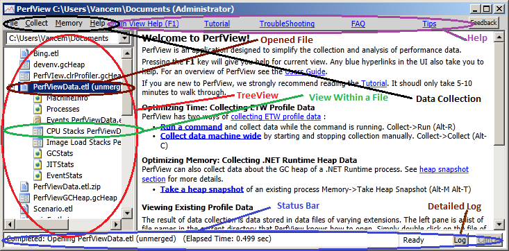
The Main view is what greets you when you first start PerfView. The main view serves three main purposes
The following image highlights the important parts of the Main View.
Typically when you first use PerfView, you use it to collect data. PerfView can currently collect data for the following kinds of investigations
The types of data PerfView understands
EventData DurationNs reveals individual pauses of each thread: this can be useful
to correlate a particular long wait to another events in the trace. Note that not all contention events
are real OS-level waits: the runtime may first spin wait to try acquire the lock fast. The metric
represents the amount of time spent to acquire the lock in milliseconds.
System.Threading.Monitor and System.Threading.Lock code paths.
WaitHandleWait events are lower level and fire when the OS-provided wait handle is used to block the thread execution.
For example, WaitHandleWait will catch waiting inside SemaphoreSlim.Wait() while Contention event won't.
WaitHandleWait can be fired alongside the Contention event: for instance, during Monitor.Enter if spin waiting
was not enough to acquire the lock. Also note that WaitHandleWait is much more noisy: you'd need to clean up
the stacks from "legit" waiting like a main thread waiting for application shutdown signal, or a consumer thread
that waits for new items in a blocking channel. WaitHandleWait may not cover all waits in your application, like waits that
bypass the dotnet runtime or waits on other synchronous OS APIs like a blocking write to a socket.
For more details, refer to this diagram from the original PR.
TODO NOT DONE
In addition to the General Tips, here are tips specific to the Object Viewer.
The object viewer is a view that lets you see specific information about a individual object on the GC heap.
TODO NOT DONE
While we do recommend that you walk the tutorial, if your goal is to understand what the stack viewer is showing you follow these steps
You can set the default value used in the GroupPats and Fold textboxes using the "File -> Set As Default Grouping/Folding" menu item. These three values are persisted across PerfView sessions for that machine. The 'File -> Clear User Config' will reset these persisted values to their defaults, which is simple way to undo a mistake.
While we do recommend that you walk the tutorial, and review Understanding GC Heap Perf Data and Starting an Analysis of GC Heap Dump, if your goal is to see your memory profile data as quickly as possible, follow the following steps
In addition to the General Tips, here are tips specific to the Stack Viewer.
The stack viewer is main window for doing performance analysis. If you have not walked through the tutorial or the section on starting an analysis and understanding perf data, these would be good to read. Here is the layout of the stack viewer
The stack viewer has three main views: ByName, Caller-Callee, and CallTree. Each view has its own tab in the stack viewer and the can be selected using these tabs. However more typically you use right click or keyboard shortcuts to jump from a node in one view to the same node in another view. Double clicking on any node in any view in fact will bring you to Caller-Callee view and set your focus to that node.
Regardless of what view is selected, the samples under consideration and the grouping of those samples are the same for every view. This filtering and grouping is controlled by the text boxes at the top of the view and are described in detail in the section on grouping and filtering.
At the very top of the stack viewer is the summary statistics line. This gives
you statistics about all the samples, including count, and total duration.
It computes the 'TimeBucket' size which is defined as 1/32 of the
total time interval of the trace. This is the amount of time that is
represented by each character in the When column.
It also computes the Metric/Interval. This is a quick measurement of how
CPU bound the trace is as a whole. A value of 1 indicates a program
that on average consumes all the CPU from a single processor. Unless that is high, your problem is not CPU (it can be some blocking operation like network/disk read).
However this metric is average over the time data was collected, so can include
time when the process of interest is not even running. Thus is typically better
to use the When column for the node presenting the process
as a whole to determine how CPU bound a process is.
In addition to the grouping/filtering textboxes, the stack viewer also has a find textbox, which allows you to search (using .NET Regular expression) for nodes with particular names.
The columns displayed in the stack viewer grids independent of the view displayed. Columns can be reordered simply by dragging the column headers to the location you wish, and most columns can be sorted by clicking on an (often invisible) button in the column header directly to the right of the column header text. The columns that are display are:
Many of the columns in the PerfView display can be used to sort the display. You do this by clicking on the column header at the top of the column. Clicking again switches the direction of the sort. Be sure to avoid clicking on the hyperlink text (it is easy to accidentally click on the hyperlink). Clicking near the top typically works, but you may need to make the column header larger (by dragging one of the column header separators). There is already a request to change the hyperlinks so that it is easier to access the column sorting feature.
There is a known bug that once you sort by a column the search functionality does not respect the new sorted order. This means that searches will seem to randomly jump around when finding the next instance.
The default view for the stack viewer is the ByName View. In this view EVERY node (method or group) is displayed, shorted by the total EXCLUSIVE time for that node. This is the view you would use for a bottom up analysis. See the tutorial for an example of using this view. Double clicking on entries will send you to the Caller-Callee View for the selected node.
See stack viewer for more.
The call tree view shows how each method calls other methods and how many samples are associated with each of these called starting at the root. It is an appropriate view for doing a top down analysis. Each node has a checkbox associated with it that displays all the children of that node when checked. By checking boxes you can drill down into particular methods and thus discover how any particular call contributes to the overall CPU time used by the process.
The call tree view is also well suited for 'zooming in' to a region of interest. Often you are only interested in the performance of a particular part of the program (e.g., the time between a mouse click and the display update associated with that click) These regions of time can typically be easily discovered by either looking for regions of high CPU utilization using the When column on the Main program node, or by finding the name of a function known to be associated with the activity an using the 'SetTimeRange' command to limit the scope of the investigation.
Like all stack-viewer views, the grouping/filtering parameters are applied before the calltree is formed.
If the stack viewer window was started to display the samples from all processes, each process is just a node off the 'ROOT' node. This is useful when you are investigating 'why is my machine slow' and you don't really know what process to look at. By opening the ROOT node and looking at the When column, you can quickly see which process is using the CPU and over what time period.
See the tutorial for an example of using this view. See stack viewer for more. See flame graph for different visual representation.
The caller-callee view is designed to allow you to focus on the resource consumption of a single method. Typically you navigate to here by navigating from either the ByName or Calltree view by double-clicking on a node name. If you have a particular method you are interested in, search for it ( find textbox ) in the ByName view and then double click on the entry.
The ByName view has the concept of the 'Current Node'. This is the node of interest and is the grid line in the center of the display. The display then shows all nodes (methods or groups) that were called by that current node in the lower grid and all nodes that called the current node in the upper pane. By double clicking on nodes in either the upper or lower pane you can change the current node to a new one, and in that way navigate up and down the call tree.
Unlike the CallTree view, however, a node in the Caller-Callee view represents ALL calls of the current node. For example in the CallTree view the node representing 'SpinForASecond' represent all instances of that function that have the SAME PATH TO THE ROOT. Thus you will see several instances of 'SpinForASecond' in the CallTree view. However if I was trying to understand the impact of 'SpinForASecond' on the whole program, it would be hard to do so in the CallTree view because it would look at all those nodes. The Caller-Callee view aggregates all the different paths to 'SpinForASecond' so you can understand quickly ALL the callers of 'SpinForASecond' and all the callees of 'SpinForASecond' over the entire program.
It is important to realize that as you double click on different nodes to make the current the SET OF SAMPLES CHANGES. When the current node is 'SpinForASecond' then this view shows ONLY samples that had SpinForASecond' in their call stack. However if you double click on 'DateTime.get_Now' (a child of 'SpinForASecond') then the view will now include samples where 'DateTime.get_Now' was called by call stacks that did not include 'SpinForASecond' and will NOT include call stacks that called 'SpinForASecond' but not 'DateTime.get_Now' . This can be confusing if you are not aware it is happening.
Sometimes you wish to view all the ways you can get to the root from a particular node. You can't do this using the caller-callee view directly because of the issue of changing sample sets. You can simply search for the node in the CallTree view, however it will not sort the paths by weight, which makes finding the 'most important' path more difficult. You can however select the current node, right click and select 'Include Item'. This will cause all samples that do NOT include the current node to be filtered away. This should not change the current caller-callee view because that view already only considered nodes that included the current node. Now however as you make other nodes current, they TOO will be only consider nodes that include the original node as well as the new current node. By clicking on caller nodes you can trace a path back to the root.
Because the caller-callee view aggregates ALL samples which have the current node ANYWHERE in its call stack there is a fundamental problem with recursive functions. If a single method occurs multiple times on the stack a naive approach would count the same SINGLE sample MULTIPLE times (once for each instance on the call stack), leading to erroneous results. You can solve the double-counting problem by only counting the sample for the first (or last) instance on the stack, but this skews the caller-callee view (it will look like the recursive function never calls itself which is also inaccurate). The solution that PerfView chooses is to 'split' the sample. If a function occurs N times on the stack than each instance is given a sample size of 1/N. Thus the sample is not double-counted but it also shows all callers and callees in a reasonable way.
See stack viewer for more.
The callers view shows you all possible callers of a method. It is a treeview (like the calltree view), but the 'children' of the nodes are the 'callers' of the node (thus it is 'backwards' from the calltree view). A very common methodology is to find a node in the 'byname' view that is reasonably big, look at its callers ('by double clicking on the entry in the byname view), and then look to see if there are better semantics groupings 'up the stack' that this node should be folded into.
If you double click on an entry in the Callers view it becomes the focus node for the callers view, callees view and caller-callees view. Thus it is fairly common to double click on an entry, switch to the Callees view, double click on another entry and switch back.
In the callers view the top node is always the aggregation of all uses of a particular method regardless of the caller. Thus the top line's statistics should always agree with the statistics in the 'By Name' view. Moreover any children of a node represent the callers of the parent node. This means
Any children in the Callers view represent callers of the parent node. These will always have an exclusive time of 0, because by definition a caller is NOT the terminal method of the stack (since it called something else).
Both the callers view and the callees view is formed by finding all samples that contain the focus frame an looking at the appropriate related node (caller or callee) related frame. However when the focus frame is a recursive function there is a because there are multiple choices for the caller and callees depending on which recursion instance is chosen.
PerfView resolves this by always choosing the 'deepest' instance of the recursive function in the stack. Thus if A calls B calls C calls B calls D, and the focus node was B, then this sample would have a caller of C (not A) and a callee of D (not C).
The callees view is a treeview that shows all possible callees of a given node. It is very similar to the treeview, but where the treeview always starts at the root, the callees view always starts at the 'focus' node and includes ALL stacks that reach that callee. In the calltree view the different instances of the node would be scattered across the call tree, and would be hard to focus on.
If you double click on an entry in the Callees view it becomes the focus node for the callees view, callers view and caller-callees view. Thus it is fairly common to double click on an entry, switch to the Callers view, double click on another entry and switch back.
Like the Caller's view there is an issue with double counting when recursive functions are involved. See Handling of Recursion in the Caller and Callees view for more.
The flame graph view shows the same data as call tree view, but using different visualization. It gives you very intelligible overview. The graph starts at the bottom. Each box represents a method in the stack. Every parent is the caller, children are the callees. The wider the box, the more time it was on-CPU. The samples count is shown in the tooltip and in the bottom panel. To change the content of the flame graph you need to apply the filters for call tree view. To learn more about Flame Graphs please visit http://www.brendangregg.com/flamegraphs.html
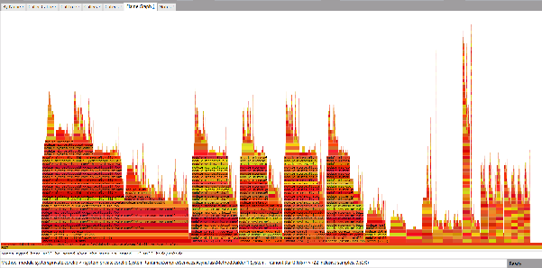
The flame graph view in PerfView traditionally reflects the amount of consumed memory, but this can change when we graph the stack differences. After garbage collection, amount of memory consumed by a type can be negative when inspected in stack differences. In those cases, the corresponding flame graph boxes are drawn with a blue hue, pointing to a memory gain. Increasing memory usage is drawn with yellow/red tint as usual.
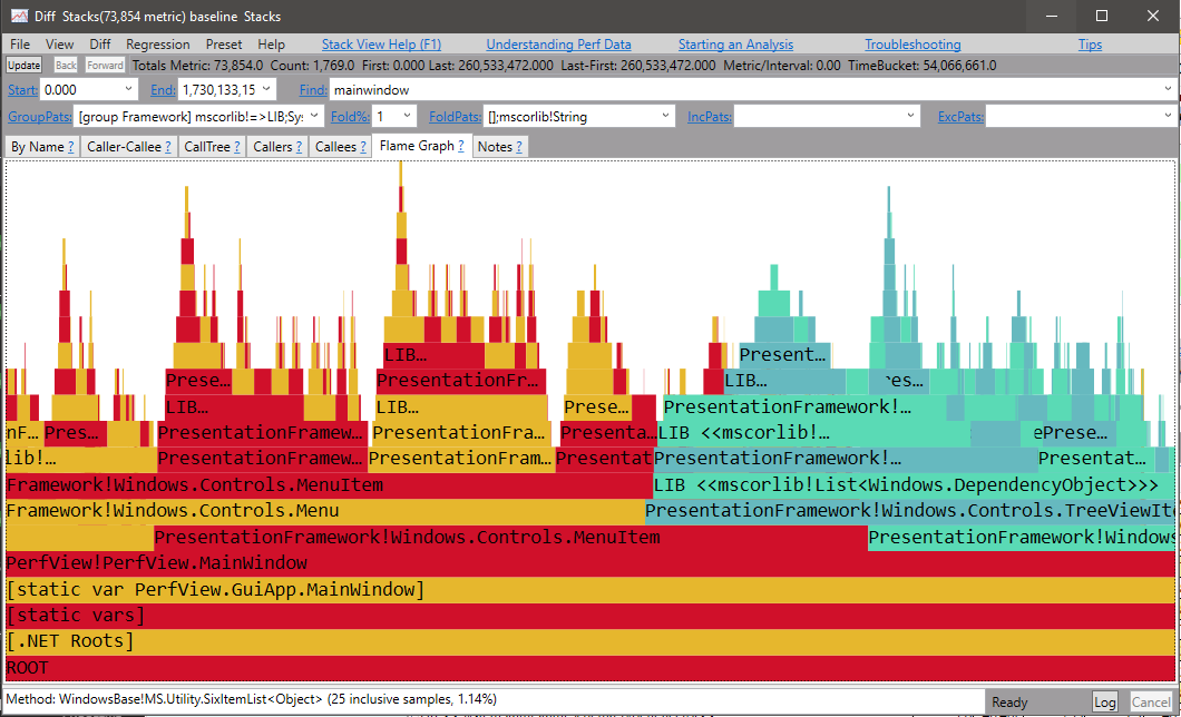
This allows you to keep notes. This view is contains the same data as in the 'Notes Pane' that you can toggle with the F2 key. These notes are saved when the view is saved, and thus allows you to keep information like the leads you need to follow up on during the investigation. The notes pane is particularly useful i you need to 'hand off' the investigation to another person. By putting the 'explanation' of the performance problem in the note pane, and sending the saved view, the next person can 'pick up' where you left off.
It is often the case that the grouping and filtering parameters definition get reasonably complex however they have a relatively simple semantic meaning. It is also useful to be able to save and reuse these parameters for other investigations. To facilitate this, filter parameter sets can be given a name (simply by entering text in the Name text box, and this name can later be used to identify this filter parameter set.
Named Parameter set are current not used by PerfView.
PerfView has the capability of taking the difference between two stack views. This is very useful for understanding the cause of a regression caused by a recent change. To use this capability you should
PerfView will then open up a stack view which contains the different between the 'test' view and the 'baseline' you selected. The algorithm it uses to do this is VERY simple. It simply negates the metric for the baseline, and then combines these samples with the samples of the test (which are unmodified). The result is a trace that has a sample which has the sum of the samples from of the 'test' and 'baseline' however the count value and metric value for all the samples in the baseline are NEGATIVE. This means that the counts and metric values will often 'cancel out', leaving just what is in the test but not the baseline.
Like a normal investigation you should start your 'diff' investigation using the 'By Name' view. In a typical investigation the 'test' trace has strictly more metric (the regression) than the baseline, and this is reflected in the totals for the diff (the total metric for the diff should be the total metric for the test minus the total metric for the baseline). The 'ByName' view then shows you where this difference came from with respect to the groups that have been selected with the 'GroupPats' (just like a normal trace).
If you are lucky, each line in the 'By Name' view is positive (or a very small negative number). This is the 'easy' case, and when this happens you have the information you are interested in (the precise groups that have additional cost in the test but not the baseline are at the top of the By Name view. From this point the diff investigation works just like a normal investigation (you can drill down, look at other views, change groupings, fold etc...)
However, it is not uncommon to have large negative values in the view. When this happens the diff is not that useful because we are interested in the ADDITIONAL time in the test trace, but the negative numbers in the view are telling us that the are big places where the baseline used more time than the test. Clearly the sum has to add up to the final regression, but as long as there are large negative values in the view, we can't trust the large positive values in the view because they MAY be canceled by the negative values.
Thus analysis of a diff trace always has an addition step: After you have formed the diff view but before you have don any analysis, you must use the grouping/folding/filtering operators to ensure that negative values have been 'cancel out' sufficiently . The view needs to have only has positive metric numbers (or inconsequential negative numbers).
In fact PerfView already helps with this. Normally a process and thread node in the stack display contains the process and thread ID for that node. While this is useful information it also means the nodes from the baseline and test trace are likely to NEVER match (since they have different IDs). If left uncorrected, this would cause the 'TreeView' to become pretty useless (it would show a large positive number under the 'test' process, and a slightly smaller large negative number under the 'baseline' but there would be no cancellation. PerfView fixes this by providing groupings that effectively remove the process and thread ID from the nodes. Now the nodes match and you get the desired cancellation.
PerfView can only do so much, however. It can anticipate the need to rewrite the process and thread IDs, but it can't know that you renamed some function, or that lazy initialization caused the cost of some initialization to move from one place to another. In short PerfView can't know all the 'expected' differences that you wish to ignore. It is your job as the analyst to make 'expected' differences 'match exactly' and thus cancel out.
PerfView's powerful folding and grouping operators are tools you will use to create this cancellation.. The mantra to remembers is 'grouping is your friend', keep your groups as large as possible. In particular
The rationale behind this strategy is straightforward. The larger the groups you form, the more likely 'inconsequential' differences will simply 'cancel out'. Modules tend to be the most useful 'big group' and thus grouping all samples by module is likely to show you a view where cancellation worked (only small negative numbers in the view). Once you identify the samples in a particular module that are responsible for the regression, you can then use the 'Drill Into' functionality to isolate JUST THOSE SAMPLES, and change the groupings to show you more detail. This tends to be a very useful strategy.
The main technique for achieving cancellation in a diff is to pick big groups and then Drill into only those samples that are of interest. However there are some other useful things to remember.
Fixing Renamed functions
Grouping lets you literally rename any node name to any other node name. Thus you can 'fix' any 'expected' differences in a trace. For example if MyDll!MethodA was renamed to MyDll!MethodB, you could add the grouping pattern
MyDll!MethodA-> MethodA;MyDll!MethodB->MethodAAl!MethodB->MethodA
which 'renames' both of them to simply 'MethodA' and resolves the diff. Folding can also be used to resolve differences like this. For example if these two methods are not event interesting (you don't need to see them on the call stacks), then you could simply fold both of them always with the folding pattern
MethodA;MethodB
which makes both of them disappear (and thus can't cause a difference).
Overweight analysis is a fairly simple technique in which the inclusive cost of all symbols from two traces are analyzed. Normally a time metric is used but any inclusive cost could work.
The idea is this: using the base and the test runs it's easy to get the overall size of the regression. Let's say it was 10%. From there you could take as your null hypothesis that everything is just 10% slower. What you're looking for is symbols that changed more than 10% and are therefore in some sense more responsible for the change. The overweight report in this case would simply compute the ratio of the actual growth compared to the expected growth of 10%. When you find symbols with greater than 100% overweight those are of great interest.
Suppose main calls f and g and does nothing else. Each takes 50ms for a total of 100ms. Now suppose f gets slower, to 60ms. The total is now 110, or 10% worse. How is this algorithm going to help? Well let's look at the overweights. Of course main is 100 going to 110, or 10%, it's all of it so the expected growth is 10 and the actual is 10. Overweight 100%. Nothing to see there. Now let's look at g, it was 50, stayed at 50. But it was 'supposed' to go to 55. Overweight 0/5 or 0%. And finally, our big winner, f, it went from 50 to 60, gain of 10. At 10% growth it should have gained 5. Overweight 10/5 or 200%. It's very clear where the problem is! But actually it gets even better.
Suppose that f actually had two children x and y. Each used to take 25ms but now x slowed down to 35ms. With no gain attributable to y, the overweight for y will be 0%, just like g was. But if we look at x we will find that it went from 25 to 35, a gain
of 10 and it was supposed to grow by merely 2.5 so its overweight is 10/2.5 or 400%. At this point the pattern should be clear:
The overweight number keeps going up as you get closer to the root of the subtree which is the source of the problem. Everything below that will tend to have the same overweight. For instance if the problem is that x is being called one more time by f you'd
find that x and all its children have the same overweight number.
This brings us to the second part of the technique. You want to pick a symbol that has a big overweight but is also responsible for a largeish fraction of the regression. So we compute its growth and divide by the total regression cost to get the responsibility percentage. This is important because sometimes you get leaf functions that had 2 samples and grew to 3 just because of sampling error. Those could look like enormous overweights, so you have to concentrate on methods that have a reasonable responsibility percentage and also a big overweight. The report automatically filters out anything with less than +/- 2% responsibility.
Most of this summary is available online with more examples here.
The Event Viewer is a relatively advanced feature that lets you see the 'raw' events collected in an ETL file. To get started as quickly as possible
In addition to the General Tips, here are tips specific to the Event Viewer.
Some data file (currently on XPERF csv and csvz files) support a view of arbitrary events sorted by time. The Event Viewer is a window that is designed to display this data. Basically it is a view of events in chronological order in time, which can be filtered and searched. A typical scenario is that the application has been instrumented with events (like System.Diagnostics.Tracing.EventSource), and these events are used to determine a time of interest.

The View has two main panels. The panel on the left contains all the events types in the trace. You simply select the ones of interest by clicking on them with the control key held down (to select several simultaneously. The right window contains the actual events records. It is relatively expensive to perform the scan over the data to form the list so you must explicitly ask for the right panel to be updated. You can do so in several ways
In addition to filtering by event type, you can also filter by process by placing text in the 'Process Filter' text box. This text is a .NET regular expression and only records with processes that match this text will be selected. The matching is case insensitive, and only has to match a substring in the process name. You can use the standard regular expression ^ and $ operators to force matches of the complete string. Note that for context switch events, the process filter will match both the process being switched from (OldProcessName) as well as the new process being switched to (ProcessName).
Traces can be very large, and thus a very large number of results can be returned in the right panel. To speed things up, on a reasonable number (by default 10000) of records are returned. This is the 'MaxRet' value. If it is too small, you can update this textbox to something larger.
In addition to filtering by process, you can also filter by text in the returned events. Only records whose entire displayed text matches the pattern will be display. Thus if you change the column's displayed it CAN affect the filtering if the there is text in the 'Text Filter' text box. The string in the 'Text Filter' is interpreted as a .NET regular expression and like the process filter by default the match only has to match a substring to succeed. If the pattern begins with a '!' character, then only entries that do NOT match the pattern will be shown.
Fields that are specific to the event are shown as a series of NAME=VALUE pairs in the 'Data' column. This data column can be quite long and often the most interested elements are at the end, making the view inconvenient. You can fix this by indicating which of these event-specific columns you wish to have displayed by placing a field names (case insensitive) in the 'Columns to Display' textbox . This can be populated easily by clicking on the 'Cols' button. This displays a popup list of all the columns, and you can simply click on the ones of interest (shift and ctrl clicking to select multiple entries), and hitting 'enter' to continue. The columns will display in the order that you selected the items, and the '*' can be used as a wild card that represents all columns that have not already been selected. A maximum of 4 fields will be displayed in their own columns. After the first 4 the rest of the specified columns will be displayed in the 'rest' column.
Events can be filtered using the Columns to Display textbox by specifying expressions combined with boolean operators: || and && based on the selected column within square brackets ([]). The format of individual queries is: LeftOperand Operator RightOperand where:
[(ThreadID == 1,240) && (ProcessName == devenv)] ThreadID ProcessorNumber [(GC/Start::Depth > 1) && (ProcessName==devenv)] [(ProcessName Contains ServiceHub) || (ProcessName Contains devenv)] ProcessName Count ProcessorNumber Depth [(Count>10 && (Depth >= -1) && (Count<=30) && (Count <= 30 || ProcessorNumber == 2))] Count ProcessorNumber Depth [(Count > 10 && (Count <= 30) && (Count <= 30 || ProcessorNumber == 2))] Count ProcessorNumber Depth The left hand panel contains all the events that are in the trace. These include the events collected by the OS kernel, as well as the .NET runtime, and any others that you indicated when you collected the data.
Because the number of event types can be large (typically dozens), there is a 'Filter' text box at the top of the event type pane. If you are looking for a particular event, simply type some part of the event name in this text box and the displayed list will be filtered to those events that contain the typed text somewhere in the name. The text you type here is really a .NET Regular expression, which means you can use wild cards (. and *) and perhaps most importantly the | operator to mean 'or'. This allow you to filter out all but some interesting events quickly. Also remember that Ctrl-A will select everything in the view.
When the event view is updated, in addition to populating the main listbox, it also generates a histogram of event counts which shows how frequency of the selected events varies over time. The time interval as designated by the Start and End textboxes is divided into 100 buckets and the event count for each of these buckets is calculated This number is then scaled so that the largest bucket represents 100% and the same convention used in the stackviewer's When Column is used to convert this percentage into a number (or letter). This displayed just above the listbox. Like the When Column you can select a portion of this display and 'zoom in' by using the 'Set Range Filter' command (Alt-R). In addition when you change the selection in the histogram text box PerfView will calculate the start and end times, total event count and average event rate and display these values in the status bar.
Here are some Kernel and .NET Events that are worth knowing more about
|
Windows Kernel/Thread/CSwitch - Shows whenever a thread either gains
or loses the use of a physical CPU.
|
Before starting collection PerfView needs to know some parameters. It fills in defaults for all but the command to run. Thus in the common scenario you only need to fill in the command to run (you are using the 'Run' command) and hit return to start collecting data.
Whether you use the 'Run' or 'Collect' command, profile data is collected machine wide. In order to collect profile data you must have administrator rights. If you do not, PerfView will try to elevate (bring up a UAC dialog box), and relaunch itself with administrator privileges.
PerfView chooses a useful default set of ETW events to log which allow common performance analysis to be done, however, there are numerous ETW events that could be turned on. Here is a sampling of some of the most useful of these more advanced events.
This option tends to have a VERY noticeable impact on performance (2X or more). Also, if the application allocates aggressively, so many events will be fired so quickly that events will be lost even when the /BufferSizeMB qualifier is used to set the size very large (e.g. 500Meg). For these reasons it is usually a better idea to use the .NET SampAlloc option instead if at all possible.
The overhead of turning on .NET SampAlloc CheckBox is much less than the .NET Alloc CheckBox. Typically the overhead is 10-20% (unlike 2X or more), and produces 200 Meg per minute of trace. This is a bit more expensive than turning on /threadTime however low enough that you can leave it on in production (especially if the application does not allocate heavily).
Note that this only affect processes that start AFTER data collection has started. This can be also activated by the /DotNetAllocSampled command line option. See GC Heap Net Mem (Coarse Sampling) for more.
The events from this option are called 'CallEnter' and show up in the 'AnyStacks' view in the 'Advanced Group' view. Most likely you will want to filter out all other events in the view by selecting the CallEnter node -> right click -> Include Item.
This option tends to have a VERY noticeable impact on performance (5X or more). If the application runs a lot of code (common), it may be necessary to make /BufferSizeMB qualifier very large (e.g. 1000Meg). and even that may not be enough This option is really only meant for small isolated tests.
There is an command line option /DotNetCallsSampled which works like /DotNetCalls, however it samples every 997 calls rather than every call. This cuts the overhead (and file size) by a factor of ~1000 which is better if overhead is a concern.
By default the runtime does not disable inlining of methods. Thus you will not see inlined calls in your trace. There is also a command line option /DisableInlining which disables inlining so you will see every call. This slows things down even more so should only be used in 'small' scenarios.
Because some of the lists use whitespace as a separator if you specify these on the command line, you will need to quote the command line qualifier.
In addition to the more advanced events there are additional advanced options that you rarely have to change.
You can select several of these options from the drop down menu and the modify the counts if desired. Currently there is no special view for these events, they show up in the 'Any Stacks Stacks' view as the PMCSample event. Thus going to that view and doing a 'Include Item' on this item will allow you to see at what stacks the samples where taken.
Note: Earlier than Windows 10 this feature does not work if there is a hypervisor enabled. If you only have 'Timer' events available this is the cause. Disable the hypervisor to use this feature.The Provider Browser is a dialog box generated from the ... button on the right of the additional providers textbox. The Provider Browser allows the user to inspect the providers that are available as well as the keywords available any particular provider.
Because there so many ETW providers available machine wide, the Browser also allows the search to be filtered to only those providers that are relevant for a particular process.
While the name of the provider and its keywords are often sufficient to decide whether what events to turn on, it is not unusual that you want more information about what the possible events are. This is what the 'View Manifest' button is for. Many providers register a XML document called a manifest that describes all the events the provider can generate in relatively fine detail. Included in this manifest is
The model for ETW data collection is that data is collected machine-wide. Moreover, data collection can exceed the lifetime of the process that started collection . While this characteristic is useful (it allows independent start and stop command line commands), it also means that it is possible to accidentally leave ETW collection running for an indefinite period of time. PerfView goes to some length to ensure that data collection is stopped in typical cases, however if PerfView was terminated abnormally, or if the command line 'start' operation was used it is possible that ETW data collection is left on. The Collect->Abort command is designed for this case. It ensures that any ETW providers turned on by PerfView are off.
Finally, is also easy to launch PerfView from the command line to collect profile data. See collecting data from the command line for more.
The memory collection Dialog box allows you to select the input and output for collecting GC Heap data as well as set additional options on how that data is collected.
Unfortunately the syntax for normal .NET regular expressions is not very convenient for matching patterns for method names. In particular the '.', '\' '(' ')' and even '+' and '?' are used in method or file names and would need to be escaped (or worse users would forget they need to escape them, and get misleading results). As a result PerfView uses a simplified set of patterns that avoid these collisions. The patterns are
This simplified pattern matching is used in the GroupPats, FoldPats, IncPats, and ExcPats text boxes. If you need more powerful matching operators, you can do this by prefixing the ENTIRE PATTERN with a @. That indicates to PerfView that the rest of the rest of the pattern follows .NET Regular expression syntax.
Simplified pattern matching is NOT used in the 'Find' box. For that true .NET regular expressions are used.
See also Simplified Pattern matching.
Fundamentally, what is collected by the PerfView profiler is a sequence of stacks. A stack is collected every millisecond for each hardware processor on the machine. This is wonderfully detailed information, but it is very easy to be not see the 'forest' (the semantic component consuming an unreasonable amount of time) because of the 'trees' (the data on hundreds or even thousands of 'helper' methods that are used by many different components). One very important tool to tame this complexity is to group methods into semantic groups. PerfView provides a simple but very powerful way of doing just this.
Every sample consists of a list of stack frames, each of which has a name associated with it. Initially looks something like this
In particular the name consists of the full path of the DLL that contains the method (however the file name suffix has been removed), followed by a '!' followed by the full name (including namespace and signature) of the method. By default PerfView simply removes the directory path from the name and uses that to display. However you can instead ask PerfView to group together methods that match a particular pattern. There are two ways of doing this.
The first form is the easiest to understanding. Basically it is just search and substitute on all the frame names. Any frame that matches the given pattern, will be replaced (in its entirety) with GROUPNAME. This has the effect of creating groups (all methods that match a particular pattern). For example the specification
Will match any frames that have mscorlib!Assembly:: and replace the entire frame name (not just the part the matched) with the string 'class Assembly'. This has the effect of grouping all methods from the class Assembly into a single group. With one simple command you can group together all methods from a particular class.
Like .NET regular expressions, PerfView regular expressions allow you to 'capture' parts of the string match the pattern and use it in forming the group name. By surrounding parts of the pattern with {} you capture that part of the pattern, and then you can use reference the string that matched that part of the pattern by using $1, $2, ... to signify the first, second, ... capture. For example
Says to match any frame that has alphanumeric characters before !, and to capture those alphanumeric characters into a $1 variable. Whatever was matched is then used to form a group name. This has the effect of grouping all samples by the module that contained them (the 'module level view').
It is useful to have more than one group specification, so group syntax supports a semicolon list of grouping commands. For example here is another useful one.
There are two patterns in this specification. The first one (in blue) looks captures the text right before the ! as well as up to the last '.' before a (. This captures the 'class and namespace' part of a .NET style method name. The second pattern does something very similar with C++ style names (that use :: to separate class name from method name. Thus the specification above groups methods by class. Powerful!
Another useful technique is take advantage of the fact that the full path name of a module is matched to group even more broadly than module. For example because * matches any number of any character, the pattern
Will have the effect of grouping any methods that came from ANY module that lives has system32 as any part of its module's path as 'OS'. This is very convenient because typically this is what people want. They don't want to see any of the details of methods INTERNAL to the operation system, they want them grouped together. This simple command does this in one swoop.
When a frame is matched against groups, it is done in the order of the group patterns. Once a match occurs, no further processing of the group pattern is done for that frame (first one wins). Moreover, if the GROUPNAME is omitted, it means 'do no transformation'. These two behaviors can be combined to force certain methods to NOT be in a group. For example the specification
Force a module level view for all modules (the red grouping pattern), however because of the first (blue) pattern, any modules that have 'myDirectory; in their path are NOT grouped by the red pattern (they are excluded). This can be used to create a 'just my code' effect. Functions of every module except the code that lives under 'myDirectory' is group together. Powerful!
The examples so far as 'simple groups'. The problem with simple groups is that you lose track of valuable information about how you 'entered' the group. Consider the example of grouping all modules in System32 into a group called OS that was considered before. This works well, but has limitations. You might see that a particular function 'Foo' calls into the OS can that whatever it did in the OS takes a lot of time. Now it may be possible simply by looking at the body of 'Foo' to 'guess' what OS function was being called, but this clearly an unnecessary pain. The data collected knows exactly which OS function was entered, it is just that our grouping has stripped that information.
This is the problem entry groups solve. They are just like normal groups but use the => instead of -> to indicate they are entry groups. An entry group creates the same group as a normal group but it instructs the parsing logic to take the caller into account. Effectively a group is formed for each 'entry point into the group. If a call is made from outside the group to inside the group, the name of the entry point is used as the name of the group. As long as that method calls other methods within the group, the stack frame is marked as being in the group. Thus boundary methods are left alone (they always form another group, but internal methods (methods that call within the group), are assigned to whatever entry point group called it.
This fits very nicely into people normal notion of modularity. While grouping all functions within the OS as a group is reasonable in some cases, it is also reasonable to group them by 'public surface areas (a group for every entry point into the OS). This is what entry groups do. Thus the command
Will fold away all OS functions, keeping just their entry points in the lists. This is VERY powerful!
Groups can be a powerful feature, but often the semantic usefulness of a group is not clear simply by looking at the pattern definition. Because of this groups are allows to have a description that precedes the actual group pattern. This description is enclosed in square brackets []. PerfView ignores these descriptions, however they are very useful for humans to look at to understand the intent of the pattern.
See also Simplified Pattern matching.
It is not uncommon that a particular helper method will show up 'hot' in a profile. You have looked at this helper method and it is as efficient as it be made. There no way to make it better. Thus it is no longer interesting to see this method in the profile. You would prefer that this method was 'inlined' into each of its callers so that they get charged for the cost (rather than it showing up in the helper). This is exactly what folding does. The 'FoldPats' text box is simply a semicolon list of patterns to fold away. Thus the pattern
Will remove MyHelperFunction from the trace, moving its time into whoever called it (as exclusive time). It has effect of 'inlining' MyHelperFunction' into all callers.
Grouping transformations occur before folding (or filtering), so you can use the names of groups to specify folding. Thus the fold specification
Will fold way all OS functions (into their parents) all in one simple command.
Generally speaking, if a method does not consume more than say 1% of the total in the view then it is usually just 'cluttering' up the display. The Fold % TextBox is designed to remove this noise. Any method whole total aggregate inclusive metric (that is what is shown in the ByName view in the 'Inc' column) is less than 1% of the total metric, is removed and its metric is given to its direct parent.
While it is tempting to increase this number to a large value (say 10% or more), to force most callstacks to be 'big' this generally produces inferior results. The reason is that the % does not take into account the semantic relevance of the node. Thus folding might fold a very semantically meaningful node into a 'helper' of some higher level function. Thus it is usually better to select nodes that 'you don't understand' to fold away so that what you are left with is nodes that are meaningful to you.
Grouping and folding have the attribute that they do not affect the total sample count in the trace. Samples are not removed, they are simply renamed or assigned to another node. It is also useful to exclude nodes altogether. The ExcPats text box is a semicolon list of simplified regular expression (See Simplified Pattern matching). If any frame in the stack matches ANY of the patterns in this list, then it is removed from the view. The pattern does not have to match the complete frame name unless it is anchored (e.g. using ^). The patterns are matched AFTER grouping and folding.
A common use of exclusion filtering is to find the 'second most problematic' performance problem in an app. In this scenario you discover that a particular method (say 'Foo') was poorly designed and you even understand how you might fix it, but you also know that is not your only problem. What you want is to find the next most important issue. By excluding the samples that call 'Foo' you can effectively simulate how the program would behave if Foo was 'perfect' (took no time). This is typically a good approximation of what the program will look like after the fix is applied. Thus by simply excluding these samples you look for the next perf problem and thus tackle many of them quickly.
By default events are captured machine wide, but often you are only interested in some of the samples. For example it is very common to only be interested in one process, or one thread, or isolate yourself to only one method. This is what the IncPats textbox does. The contents of the text box is a semicolon separated list of simplified regular expressions (see Simplified Pattern matching). It is required that a stack matches at least ONE of the patterns in the IncPats list for it to be included in the trace. The pattern does not have to match the complete frame name unless it is anchored (e.g. using ^). The patterns are matched AFTER grouping and folding.
As mentioned, it is very common to use the IncPats textbox to restrict your analysis to a single process. It is also very useful to use the '|' (or) operator here so that you can include just two (or more) processes and exclude the rest.
It is very useful to 'zoom in' to a particular time of interest and filter out samples outside this range. This is done by setting the 'Start TextBox' and 'End TextBox' appropriately. These ranges are inclusive (on both ends), and are expresses as msecs from the start of the trace. You can of course enter times manually or cut and paste numbers from other parts of the display. In addition if you paste two numbers into the 'start' textbox it will set both the start and end values. There are a few other nice shortcuts for setting a time interval.
The 'First' and 'Last' columns of tree node are often a useful range to filter on. To do this easily, simply select both the boxes (either by dragging or by holding the 'Ctrl' key as you click additional entries), Once you have selected two cells you can right click and select 'Set Time Range' which will set both the start and end time to the first and last column. You can also select a time range by coping two numbers to the clipboard (select two cells and press Ctrl-C) and then pasting the numbers into the 'Start' textbox. This textbox is smart enough to recognize that the pasted value is a range and will set the 'End' time appropriately.
It is also very useful to select time ranges based on the 'When' column. To do this, first select a 'When' cell of interest. This will cause the status bar at the bottom of the view to display the 'When' text. By dragging the mouse over the characters, highlight the region of interest (it is typically the region of high cost). Then move your mouse off the selected region, right click and select 'Set Time Range'. This will set the 'Start' and 'End' time to the region you selected. You may end up repeating this process to further 'zoom in' to a region.
If there are more than 1M data samples being viewed in the stack viewer, the responsiveness becomes very sluggish (it takes 10 > seconds to update). To avoid this some stack source (most notably the memory stack source), support the concept of sampling. The basic idea behind sampling is to only process every Nth sample. Thus by setting the sampling text box to 10 the stack view will only have to process 1/10 of the data and thus should be 10 times faster. When Sampling is enabled, the stack-viewer automatically scales all counts (and therefore metrics too) in the view by the sampling rate. Thus the resulting metric and counts are approximately the same as without sampling (you can see this because all counts are a multiple of the sampling rate.
Text searches of names in the view can be performed by typing a search pattern in the 'Find:' text box in the upper right corner of the stack viewer. Ctrl-F will bring you to this search box quickly. The search pattern uses .NET regular expressions, and is case insensitive. Searching starts at the current cursor position and will wrap around until all text is searched. The F3 key can be used to find the next instance of the pattern. When all the text has been searched the app will beep. The next F3 after that starts over. Specification of expressions combined with boolean criteria can be done similar to filtering select columns in the Columns to Display textbox.
GroupPats, FoldPats and Fold% text boxes can be edited to contain custom patterns. These patterns combined together can be saved as a named preset.
In order to create new preset use Preset -> Save As Preset menu item. If GroupPats text box contains description (enclosed in []), then the description will be offered as a preset name. Otherwise automatically generated name will be suggested.
All created presets are added to the Preset menu for all active PerfView windows. Select menu item in the Preset menu to activate a preset. The name of the preset will be shown in [] in the GroupPats textbox. Presets are saved across sessions. Preset -> Manage Presets menu item allows editing existing presets as well as deleting them.
Wall clock time investigations break down into two cases. Either most of that wall clock time is dominated by CPU (in which case a CPU investigation is will work), or it is not dominated by CPU time, in which case you also need to understand the blocked (non-CPU) time being consumed. Thus the 'hard' part' of doing a wall clock investigation is understanding blocked time.
Blocked time investigations are inherently harder than CPU investigations. CPU investigations are reasonably straightforward because in most scenarios any CPU usage is 'interesting' to investigate regardless of where it happens. Thus the trivial algorithm of attaching the same weight to every msec of CPU regardless of where it happened is appropriate. This is actually not true in some scenarios. For example, if there was a background CPU-bound task on a multi-processor machine, the CPU associated with that background task is likely not very interesting because it is not consuming 'precious' resources and is not on the critical path of some user operation. Thus if you were investigating CPU on such an application you would need a way of filtering out this 'background' activity so you could concentrate on the 'important' CPU use. Typically this would be easy to do because the threads that execute such background CPU activity are dedicated to background activities (so you can just exclude all samples from those threads). However imagine if the background thread was a 'service' and important foreground CPU activity was scheduled on it interleaved with the idle background activity. This would make analysis quite difficult.
This bad situation is EXACTLY the situation you have with blocked time. Typically there are many threads that spend most of their time blocked, and most of this blocked time is never interesting because it is not part of a critical path. However these threads wake up at least some of the time and PARTS of their execution can be on the critical path (and thus are very interesting). Unfortunately is no simple, general way of separating 'important' blocked time (on a critical path), from uninteresting blocked time without additional 'help' (annotation) of the INTENT of the program. Thus the 'trick' to doing a blocked time analysis is to use scenario specific mechanisms to tag the 'important' blocked time and allow it to separated from the (large amount) of unimportant blocked time.
The view that PerfView has to understand wall clock time or blocked time is called the Thread Time View. This view is based on the observation that at any instant in time every thread is doing 'something'. It might be consuming CPU, or it is not (which we will defined as BLOCKED). If it is BLOCKED it might be because it waiting for its turn to use a processor (which we call READIED), or it may be waiting on something else (e.g. for a DISK request to respond, or the NETWORK to respond or for some synchronization object (e.g. Event, Mutex, Semaphore ...) to change state. Whatever it is doing there is a stack associated with it. Thus at every instant of time every thread has a stack and that stack can be marked with a metric that represents wall clock time that the thread consumed at that call stack. This is a 'perfect' model of what every thread is doing on the system.
If you set the 'thread time checkbox on the collection dialog, or pass the /ThreadTime qualifier to the command line, PerfView will ask the operating system to collect the following information:
With this data we have 'perfect' information on where we are blocked. We know the exact time when we started to block and when we ended, and thus can attribute exactly the correct amount of time to that particular stack. We also have approximate information where CPU time is spent. If we get a sample (which might be a CPU sample or a context switch) we can attribute that stack with the time spent since the last sample was taken (which again is either a context switch (e.g. if the thread had the CPU less than 1 msec) or another CPU sample (e.g. if it has been longer than 1msec since the last context switch). Thus the events above we can do a VERY good job of detailing exactly where each thread spent its time. It is interesting to note that you get 'perfect' information on EXACTLY how much CPU time things use (since you know exactly when threads start consuming CPU time and when they stop consuming CPU). The only imperfection is that the stacks associated with CPU is only a sampling.
This transformation of context switch and CPU samples is the foundation of the 'Thread Time Stacks' view in PerfView and is the view of choice to understand wall clock time (or blocked time). Like the CPU stacks view, the Thread Time Stacks view shows inclusive 'tree' which aggregates all these stacks of where threads spend their time. At the bottom (away from thread start) end of each stack a pseudo-frame is appended which indicate what information is known about that stack (CPU_TIME, DISK_TIME, HARD_FAULT (disk time to fetch mapped files), NETWORK_TIME, READIED_TIME or BLOCKED_TIME). For some things more is known (like the file or network port, so pseudo-frames get inserted for those too. These tags make it easy to use PerfView's folding and grouping and filtering capabilities to look at only certain causes of delay.
In broad strokes, a clock time investigation consists of the following steps
To recap, a Wall clock (or blocked time) investigation always starts with filtering to find 'interesting' wall clock time (typically on a single thread). Until you get to this point you can't sensibly interpret the 'Thread Time View', but after you have found the interesting time, it proceeds much like a CPU analysis.
Sometimes identifying the size and call stack of blocked time is sufficient to understand a particular performance problem. For example analyzing the cold startup time of an application falls into this category because understanding why the blocked time is as long as it is is clear (a Disk read was needed), and so the only questions are how long are these operations and where did the occurred (what stack caused them). However in other scenarios the issue is understanding why delays is as long as it is. For example, if a thread is blocked waiting on a lock, the interesting question is why was some other thread holding the lock so long? To answer this question you need to determine which thread was holding the lock. Questions like this are what the ReadyThread event helps answer.
When you you turn on the /ThreadTime events, not only do you turn on the context switch events, you also turn on the ReadyThread events. A ReadyThread event fires when one thread causes another thread to change from being BLOCKED to being runnable (that is it make a thread READY to run). Thus if thread A is waiting on a lock that thread B owns, when thread B releases the lock it make thread A ready to run. When a ReadyThread event fires in this example it logs both threads A and B as well as the stack of thread B. Loosely speaking, READYTHREAD logs the fact that thread B CAUSED thread A to wake up.
PerfView has a special view for displaying READYTHREAD information called the 'Thread Time (with ReadyThread)' view. This view works just like the 'Thread Time' view but in addition, every stack where a thread blocks is 'extended' with additional frames that tell you the thread and stack that woke it up. These extra frames are suffixed with '(READIED_BY)' so that you know that you can easily see these are not ordinary frame (and you can fold them away if you like). In the example of a Thread A waiting on a lock and being awakened by Thread B releasing the lock you would see
Which clearly shows that after blocking in 'X!LockEnter' the thread was awakened by thread B calling 'X!LockExit'.
If you have not already read the basics of Understanding Thread Time you should read that now. This section builds on those basics.
It is strongly recommended that if you need to do asynchronous or parallel operations, that you use the .NET System.Threading.Tasks.Task class to represent the parallel activity or the 'continuation' of the thread after an asynchronous operation completes (the 'await' feature in C# uses Tasks). What makes Tasks valuable to PerfView is that this class logs events when Tasks are created (along with an ID for the created task), when there body of the task is invoked (along with an ID for the task), and when the task's body completes (again along with an ID). This helps us in two important ways
The 'Thread Time (with Task)' view does exactly this. When a thread calls a task creation method, this view inserts a pseudo-frame at this point that indicates that a task has been scheduled, and then inserts all the events for the body of that task at that point . Here is an example
In this example the 'Main' Program called 'DoWork' which had the code
This call causes another thread (in this case thread 848 to start up, and start executing the body (the delegate {...}). This 'inline delegate' code is called an anonymous delegate, and the C# compiled generates name for it (in this case 'c__DisplayClass5.<DoWork>b__3'), which does the the work (note PerfView's 'Goto Source' (Alt-D) option is VERY handy at this point for seeing exactly what this code is).
The important part here is that from a source code level it is very natural to think that any costs (time) spent in this anonymous delegate should be 'charged' to 'DoWork' because that code caused that delegate to actually run (on a different thread). This is EXACTLY what the Thread Time (with Tasks), view does. If your application uses Tasks, you should be using this view.
At its heart, a server investigation is typically about response time. Thus to do an server investigation you would like all costs that contribute to making this response time longer rolled up together in the display. This is exactly what the Thread Time with Start-Stop Tasks View does.
This is best shown by example. This is an example of a ASP.NET Web server that was monitored using 'PerfView /threadTime collect'. Because we use the /ThreadTime parameter, information on context switches and tasks is collected that allows 'Thread Time' views to be displayed including the 'Thread Time (with StartStop Tasks)' display . Here is the result of opening this view and focusing on the W3WP process (which is the web server process).

At the top of the tree, we see the process node, but then immediately all costs are segregated into two parts, things that are associated with some start-stop activity, and everything else. Thus this lets you quickly focus on the thread time that is likely to be of interest.
Under the 'Activities' node you see all 'top level' start-stop activities, sorted by cost (that is thread time attributed to that activity). In the view above we opened the 'IISRequest' activity (which has a particular ID number and URL) that happens to have 730.7 msec of thread time. This IISRequest Activity happens to cause another nested Start-stop pair for an AspNetReq activity, so that is shown, from there all stacks associated with the AspNetReq activity are shown. In this example we can see the call stack through user code to the method MyOtherAsyncMethod which does a 'await' that takes 524.5 msec)
Hopefully you can immediately see how useful this view is. Basically it takes all the thread time associated with semantically relevant things (start-stop tasks that someone instrumented into the code), and displays the stack based on causality (thus event if execution hops threads the stacks 'follow' it). Thus it becomes trivial to see exactly where time is being spent.
A typical strategy is to immediately select the '(Activities)' node, right click -> Include Item, which will exclude all the non-activity thread time. This works well most of the time however keep in mind that some important costs may be in this (Non-Activities) node, in particular things like the GC (in server or background GC), or any non-threadpool threads did work but never logged a start and stop event. This is why PerfView does not hide this, but typically you start by looking at the activities, only look outside that if you are lead there. Typically if you will filter to just look at the non-activities and only the CPU_TIME, to see what is 'interesting' in that group.
It is important to note that what is being shown is STILL thread time, NOT wall clock time. Thus if there is concurrency going on, the total metric is very likely to add up to more than elapsed wall clock time. This is easy to determine this is the case (because you will see more than one thread as children of the activity), and you can even see the overlap (by looking at the 'when' column of each of the children). Still it is something to be aware of. See Understanding Thread Time and for more.
It is also possible that the thread time will be LESS than elapsed wall clock time. This should be a much rarer case. It happens when the code causes work to happen but does not use the mechanisms that have been instrumented to detect that work on another thread was caused by the current thread. Because of this the current thread may return to the threadpool (at which point its time is NOT attributed to the activity anymore), but because the work on the other thread is unknown to PerfView, it can't properly attribute that time to the activity (it ends up under the non-activities node). Thus there can be 'gaps' in the thread time for a request. PerfView tries to fill these gaps with a pseudo-node called 'UNKNOWN_ASYNC', so that at the cost in the view is never less than the wall clock time for sorting purposes, but sometimes PerfView's algorithm is not perfect. In either case, however it becomes very difficult to determine what was going on during these gaps. Hopefully this simply won't happen to you...
Often the 'standard' instrumentation in the .NET Framework gives you good 'starting' activities to work with (as the IISRequest and AspNetReq did above). However if those are not sufficient, you can define start-stop activities of your own. If your code is running on V4.6 of the .NET Framework or beyond, then it is trivial to add new start-stop activities that will show up in this view. See EventSource Activities for details of doing this. You will want to turn your events on using the /Provider=*YOUR_EVENT_SOURCE_NAME when collecting data, and this view will simply incorporate them automatically.
PerfView can also be used to do unmanaged memory analysis. Typically the first step in a memory investigation (whether it be a managed or unmanaged memory investigation is to use a tool like the free SysInternals vmmap tool to determine what the memory make up is of your process. This tool can break down the current memory usage into half a dozen categories including
Depending on which of these is big (and thus interesting, you attack it differently. If mapped DLLs or EXEs are the issue, you need to load fewer of them. PerfView's 'Image Load Stacks' will show you where you are loading DLLs. If the problem is GC Heap, you need to do a GC Heap investigation as described in 'When to care about the GC heap'. If the problem is either of the last two, then this section tells you how to drill into that problem.
In the end, all memory in a process is either mapped (e.g. DLLs or EXEs) or is allocated by windows VirtualAlloc API. PerfView allows you to collect a stack trace on every VirtualAlloc call (and every VirtualFree call), by checking the 'Virtual Alloc' checkbox on the advanced collection dialog box. VirtualAlloc was designed to be used to allocate large chunks of data (in fact the minimum size is 64K), and so turning this option on is not likely to affect the performance of your app, so feel free to do so. However precisely because VirtualAllocs are called infrequently (typically when another allocator needs more memory), this information is often 'to coarse' and is only useful when your user code directly calls this API (which is unusual).
Much more commonly, you will notice in your VMMAP the that 'Heap' entry in the display is large, and thus you want to drill into the OS heap. To do this we need to collect data every time an OS heap allocation or free happens. This is MUCH more common. In fact it is so common that the operating system does not provide a way to turn it on system wide (that would be too much data) instead there are two dialog boxes in the advanced section of the collection dialog box.
Using one these two techniques you can turn on OS heap events for the process of interest. Optionally you can also turn on VirtualAlloc events.
Once you have done this and collected data, you will get the following views
The two views work the same way. Every allocation in the trace is given a weight equal to the number of bytes allocated. Every free is given a negative weight and and the CALL STACK OF THE ALLOCATION (this way they perfectly 'cancel out'). Frees that can't be matched up with allocations in the trace as a whole are ignored. After this PerfView treats the stacks just like any other stack-based data it processes. It only considered samples that match its filters and displays the result. Note that this means that VALUES CAN BE NEGATIVE. If you select a time rage where only frees happen then you will get a negative number. The basic invariant is that the view shows you the NET memory allocation for the range you select. Because metrics can now be negative the 'When' column might need to show negative numbers. These are displayed by using lower case letters (see When Column for more).
Note that this means that if you display the TOTAL execution of a program in theory you should see a value of 0 (you freed everything you allocated). In practice this is not true but what IS true is that you are not usually interested in the FINAL memory used just before process termination, but the PEAK memory allocation. To get that you need to find the time where memory allocation was at its peak.
You can do this (roughly) by going to the ' CallTree View' and selection the When Column for the root of hierarchy. As you drag regions of the when column PerfView will compute the net and peak metric in the region that you dragged. Thus by dragging you can quickly determine where the peak is. Typically you the simply need to hit 'Set Range' (Alt-R) and now you have the region of time where you built up to the peak memory usage.
You can also easily investigate the net memory usage of any particular operation by selecting the time rage over that operation. All the normal filtering, folding and grouping operators work. for the memory case. Finally by opening two views you can use the Diff feature to do an analysis of two runs of the application.
The directory size menu entry will generate an *.directorySize.perfView.xml.zip file that is a hierarchical summation of the sizes of all files in a directory (recursively). Thus it is a very good tool for determine what is taking up disk space on a disk drive and 'cleaning up' less valuable files.
Selecting this menu entry will bring up a directory chooser that you use to select the directory to analyze as well as the name of the file that will hold the gathered data. Once selected PerfView will do a recursive scan on that directory which make take a while. When it finishes (which may take a while for large directories), it will automatically open the data file it generates). You may reopen the file at any time later simply by clicking on it in PerfView's main tree view.
The 'when' field for directory size works a bit different than for most performance data. For each data file, its 'Timestamp' is the number of days (which can be fractional) from the time that the data was collected, to the time it was last modified. Thus by selecting the time range from 0 to 7 you will see all files that were modified less than one week ago. This information can be very useful for seeing how 'old' the data is (which is often useful to determine whether to keep it or not).
Selecting the Size -> Image Size menu entry will bring up a dialog box you use to specify the DLL or EXE to do the size analysis one. In addition it will allow you to set the name of the output file that holds the resulting data. The dialog will derive a output file name from the input file name and generally this default is fine.
The image size menu entry will generated a .imagesize.xml file the describes the breakdown of the size of a DLL or EXE file. It does this by looking up every symbol for the DLL/EXE in its PDB file and using those names for each chunk of the file. It also looks for references from on part of the file to another (for example pointers in memory blobs or assembly code to other memory blobs or assembly code. Because these references can form arbitrary graphs of dependency in the same way the GC heap objects form a graph of dependency, PerfView displays this data in very much the same way as a GC heap. Like a GC heap, the 'When', 'First' and 'Last' columns do not show the time but represent an address of where the particular item is in the virtual address space when loaded. Thus you can also use this to get an idea of the locality of different symbols within the file when loaded.
As mentioned, by default PerfView tries to create a 'GC heap' of the items in the DLL if one item refers to another it will have a link from the referencer to the object being referenced. However this behavior can interfere with some analysis. . In particular if you use the 'include pats or 'exclude pats' textboxes, it will include or exclude ON THE ENTIRE PATH. When this is not what you want, one easy way to fix the problem is to 'flatten' the graph.
Flattening a set of nodes takes one set of nodes, and returns a new 'GC Heap' where
Many of the names used in the image size report are the symbol names that symbolic names that have a direct relationship with the names in the source code. However other names describe entities of the Portable Executable (PE) format which are needed to prepare the code/data in the DLL/EXE to be run. Here we describe some of these that may show up prominently in the output.
Other names are associated with the .NET Runtime Native file format.
Selecting the Size -> IL Size menu entry allows you to do a analysis of what is in a .NET Intermediate File (IL), which is what .NET Compilers like C# and VB create. It will generate a .gcdump file that makes graph of types, methods, fields and other structures in the IL file where each node of the graph indicates how big it is in the file, and the arcs between the nodes are references from one item to another. Thus you can do dependency analysis (what things refer to what other things), in the same way as objects in a GC heap.
The Size -> IL Size menu entry will bring up a dialog box you use to specify the DLL or EXE to do the size analysis on. This file needs to be a DLL or EXE that contains .NET IL (e.g. the output of a .NET compiler). In addition it will allow you to set the name of the output file that holds the resulting data. The dialog will derive a output file name from the input file name and generally this default is fine.
The image size menu entry will generated a .gcdump file the describes the breakdown of types methods fields and other items in the IL file. It works in much the same way as the GC heap analysis or the native Image Size Analysis.
The Menu entry only allows you to specify one IL file when creating the node-arc graph for the IL code. Any references outside this file are not traversed, but simply marked as a special 'external reference' node. It is sometimes useful to select a group of IL files (e.g. representing a complete application) which are traversed and only when you leave this group would you use 'external reference' nodes. You can do this with the 'ILSize.ILSize' user command. Thus the command
Will create a GC heap of File1.dll File2.dll and File3.dll as if they were one file.
Often, it is useful to analyze performance of one program across multiple traces. These traces might represent one large project in a variety of scenarios, or the behavior of a common library being used by multiple programs. PerfView supports several features for this sort of multi-scenario analysis.
A main challenge when doing analysis of multiple scenarios (data files) simultaneously is simply the quantity of data being manipulated. Individual scenarios can often have an ETL file that is 100s of megabytes, and and if you have 100 such scenarios you are now talking 10-100 GB of information to process. Because of this, the process is designed to reduce the data volume as quickly as possible and to persist this 'lean' form so that the data volumes at viewing time are kept under control. Thus there are two main steps in working with a multiple multiple scenarios
The following is more detailed instructions on performing these steps.
The first step in viewing multiple data file simultaneously is to preprocess the data into a 'Scenario Set'. You can do this with the 'SaveScenarioCPUStacks' user command(currently only CPU sampling aggregation is supported). You can run it from the PerfView GUI using the 'File->UserCommand' menu item or from the command line by executing the following
The SaveScenarioCPUStacks command takes one argument. This argument
can be a directory name (as in the example above), or the path to an XML config file.
If you pass in a directory, SaveScenarioCPUStacks will run in "automatic" mode.
It will process all ETL and ETL.ZIP files found in the directory (or any sub-directory),
using a heuristic method to automatically detect the process of interest for the
trace. The heuristic used to pick the process of interest is
Typically this heuristic approach works well, however if you need control over how SaveScenarioCPUStacks
runs, you can pass in an XML configuration file that gives you fine control over the processing of the ETL files.
Here's an example XML config file:
<ScenarioConfig>
    <Scenarios files="*.etl" name="Win8 Store scenario [$1]" />
    <Scenarios files="ScenarioProcess.etl.zip" name="PerfView" process="procexp64"
         start="1000" end="5000" />
</ScenarioConfig>
As you can see, a config file is composed of a root ScenarioConfig
element, which contains one or more Scenarios elements. Each Scenarios element
has attributes set that control how scenarios are processed:
files attribute is the only required attribute of the Scenarios element . This attribute's
value is a wild card pattern of files to match. All files matched by this pattern
will be preprocessed and included in the output scenario set. (Relative paths are
relative to the directory containing the XML config file.)
name attribute controls the name of the scenario, as it is displayed
in the GUI. This can contain $-substitutions as specified in the .NET framework documentation.
Each * in the wild card pattern will be converted to a capture group,
which will allow its use with the $number substitution. (For
example, the first * in the pattern can be referred to as "$1".)
process attribute allows you to override the process-of-interest
detection logic for a trace. The value of this attribute should be the name of the
process you wish to include (without any .exe file extension). If you use '*' as the process name then all processes from the trace are processed into the perfView.xml.zip file. Like the 'name' attribute you can use $1 in this attribute which will be replaced with the corresponding capture group.
start and end attributes allow you to set the time
range of interest from the matched traces. Events at time start will be will be at
time 0 in the processed output, and any events outside of the time range will be dropped
The result of running the SaveScenarioCPUStacks command are the following output file.
*.perfView.xml.zip file for every trace matched. These will
only be generated if they do not exist, or if their corresponding ETL trace data is
newer, but if they are up to date, nothing is done for that file.
*.scenarioSet.xml file for the entire scenario set.
This file is necessary for the viewing the data in step 2.
If you'd like, you can also generate your own scenarioSet.xml file.
A scenarioSet file is similar to a scenario config
file, but with slightly different attributes. Here is an example scenarioSet file:
<ScenarioSet>
    <Scenarios files="*.perfView.xml.zip" namePattern="Example scenario [$1]" />
    <Scenarios files="foo.perfView.xml.zip" namePattern="Example scenario [baz]" />
</ScenarioSet>
As you can see it is basically a list of file patterns (which indicate which files in the directory (or any subdirectory) of the directory holding the ScenarioSet.xml file should be included), as well as a pattern that allows you to take that file name and convert it to scenario name. You can make your own XML files to create interesting subsets of some data.
Once you've processed your scenario data, you can then proceed to view it. To do this, use the treeview in the main view to browse to the generated scenarioSet.xml data file and double-click to open it.
For the most part, this is the familiar Stack viewer you use on a single ETL file, the main difference is that each stack from a particular data file (scenario) has a new pseudo-frame at the very top that identifies the scenario that the sample comes from. Thus stacks belong to threads belong to processes belong to scenarios. Everything else about the stack viewer works as it did in the single-scenario case. The stack view appears as if every scenario simultaneously on the same machine.
In addition to the new 'top' node for each stack, the viewer has a couple of enhancements that only are visible in the multi-scenario case. You will see:
In the same way that the 'when' column allows you to see for every row in the view a small graph displaying the samples as function (histogram) in time, the 'which' shows you a histogram of the scenarios that had samples contributing to that row. Thus you can quickly determine whether the cost of that row was uniformly distributed across scenarios or whether just a handful of scenarios contributed to the cost.
The which field has a number of handy features associated with it.
PerfView uses the Event Tracing for Windows (ETW)Windows (ETW) facility built into windows to collect profiling information. This infrastructure does not naturally create a single file for the data, but segregates data that came from the OS kernel from other events. Thus the 'raw' data generated consists of two files (one which is just etl, and another .kernel.etl). Moreover these files are missing some information that is needed to fully decode the file on another machine (most notably, the mapping of OS kernel names to NTFS file names and the symbol server 'keys' that allow unambiguous lookup of symbolic information (PDBs). Neither of these limitations are a problem if you consume the data on the same machine as it was collected on, but if you wish to transfer it to another machine, you should first merge the data.
Merging is a process by which the .kernel.etl is merged into the main .etl file. In addition the missing system-specific information is gathered up and also placed in the .etl file. The result is a single file that can be copied to a different machine for analysis. This process can take a non-trivial amount of time (10s of seconds), which is why PerfView does not do it by default. You can perform merging by
Once the file is merged, you can simply copy the single file to another machine for 'off-line' analysis. Note however that while the ETL file contains symbolic information for .NET Runtime code, it does NOT contain symbolic information for unmanaged code. Thus if it is important to see the symbolic names for unmanaged code, you need to ensure that the machine on which analysis occurs has access to the PDB files that contains this information.
Merging an operation necessary to view ETL files on a machine other than the machine the data was collected on. However it is not sufficient for all cases. While the resulting merged file has all the information to look up symbolic information (for stack traces), it does not guaranteed that the symbolic information will be available. In particular, when collecting traces whose processes use the .NET runtime, it is necessary to reference the symbolic information (PDB files) for the native code images (NGEN images), of the managed code (if it was NGENed). These NGEN Pdbs are NOT the PDB file for the IL images (something created by IL compilers like CSC.exe, or VBC.exe). The NGEN PDBs are generated by the NGen.exe command that comes with the .NET framework and can only be reliably generated on the machine that generated the NGEN image.
As part of the ZIPPing process, PerfView will look up all addresses in the ETL file and determine which NGEN images were used, and if necessary generate the PDB files for those images. It will then ZIP both the ETL file as well as any NGEN PDBs into a single ZIP file that can now be viewed on any machine (PerfView knows how to automatically unpack these files).
See also PerfView Extensions for advanced automation by building an extension for PerfView.
See also Command Line Reference for a complete list of the options you can use at the command line
PerfView is designed so that you can automate collecting profile data be using a batch file or other script. The three likely scenarios are:
In the first case you are likely to want to use either the 'run' or 'collect commands
The 'run' command immediately runs the command and launches the stack viewer. This is the preferred option if it is easy to launch the program and it can be run to completion. However sometimes it is difficult to do this (the app is part of a service, or is activated by a complicated script), then you can start system wide collection with the 'collect' command.
By default the 'collect' command performs a 'rundown' where information to properly decode symbolic information collected before profiling stops. This operation can be relatively expensive (takes seconds, and increases file size by 10s of Meg). This information is naturally provide when processes shut down, but the 'collect' command does not know if you shut down the process of interest, so it performs the rundown. If you know that the process of interest has exited, then rundown is pointless and can be avoided by specifying the /NoRundown qualifier. This option can save time and file size.
By default PerfView assumes you wish to immediately view the data you collected, but if the person collecting the data (e.g. a tester) is not the person analyzing the data (e.g. a developer), then we wish to suppress the viewer. This is what the /noView qualifier does and it works on the 'collect' and 'run' command. Thus
Will turn on logging and run the given command. It will also merge the file, under the assumption that the file is likely to be moved off the current system. It will however still bring up the GUI and it will not exit automatically when it is done (so that the user can react to any failures or messages and is required for the 'collect' command so that the user can indicate when collection should stop).
See also Command Line Reference for a complete list of the options you can use at the command line
The /NoView makes sense where is it hard to fully automate data collection (measuring ad-hoc scenario in a GUI app). However for fully automatic collection you don't want the GUI at all. This is what the /LogFile qualifier is for. By specifying this qualifier you indicate that no GUI should be opened and that the program should exit after running the command on the command line. Any error messages that would have been reported in the GUI instead are APPENDED to the log file (we append so you can use the same file for several PerfView commands. The exit code of the PerfView process will indicate the success or failure of the collection and the log file will contain the detailed diagnostic messages.
Note that the /LogFile qualifier will suppress the GUI, but it will not suppress the generation of a console if the 'Collect' command is specified and no /MaxCollectSec qualifier is given. The reason is that without /MaxCollectSec=XXX the Collect command could run forever and you would have not way of stopping it cleanly (you would have to kill the process). If you wish to use /LogFile and Collect (because you wish to use the /StopOn* qualifiers), and wish to suppress any consoles, you can do this by specifying a very large /MaxCollectSec value.
In addition to the /logFile qualifier it is good to also apply the /AcceptEula qualifier to scripts that call PerfView. By default the first time PerfView is run on any particular computer it displays a pop-up that asks the user to accept the usage agreement (EULA). This can be problematic for scripts since it requires human interaction. To avoid this you can use the /AcceptEula qualifier on the command line that does this operation silently.
Thus a typical use of the /logFile and /AcceptEula qualifiers is the command
which runs the 'tutorial.exe' from a script (no GUI). If you need to collect system wide, (you want to use 'collect' not 'run') there is a problem because PerfView does not know when to stop. There are two ways to solve this problem. The first is to use the '/MaxCollectSec' qualifier.. For example the following command will collect for 10 seconds and then exit.
If you wish to control the stopping by some other means besides a time limit, you can also use the 'start' and 'stop' and 'abort' commands.
These are meant to be used in scripts. The first will start logging and leave it on even after program exit. The second stops logging. You should avoid using these (use collect /MaxCollectSec instead), if you can. The reason is if the script where to fail between the start and stop commands, logging might not be stopped and will run 'forever'. Thus some care is necessary in using these. The 'abort' command is meant to help ensure that PerfView is not logging. It is meant to be called at locations where you know that PerfView should NOT be running, and it ensures that indeed it is not. You should use it liberally in scripts that use the 'start' command.
The normal Event Tracing for Windows (ETW) logging is generally very efficient (often < 3%) however after a trace has completed, PerfView normally does relatively expensive things to package up the data (including merging, NGEN symbol creation and ZIP compression). These operations obviously can use resources that may slow down whatever else is running on the machine.
If you pass the /LowPriority option to PerfView on the command line, it PerfView will do these operations at low CPU priority. This can significantly slow down the time it takes to package up the data, but it minimizes the impact to the system.
Containers can be best thought of as a light weight virtual machine. See Windows Containers on Windows 10 for more background on containers for windows. In particular windows supports a light weight container called a 'Windows Server Container' in which the kernel is shared among all the containers running on a machine. Such containers are used in conjunction with a tool called Docker, which allows you to create OS images and run applications in the virtualized environment.
Ideally containers should be irrelevant to using PerfView, since containers are a kind of windows operating system and PerfView is just a windows application running there. This is mostly true, but there are some differences that need to be considered.
Thus PerfView works in a container, but need to ensure you have a new enough version of the operating system, and that you use the techniques in Automating Collection to collect data without using the GUI.
A example is worth a thousand explanations, so here is an example. First you need to set up install Docker for windows from the web. There are plenty of good tutorials on line for that. Once you have docker set up you can do the following
which will pull down the 1803 version of Windows Server Core (it is about 5GB) and run the 'cmd' command in it. Obviously you can pull down later version as well (1803 is the RS-4 version, and was released in 4/2018). The important part is that it is RS-3 or later. The result is a C> command prompt.
At this point you can copy PerfView into your container (e.g. 'net use \\SomeShare\SomeSpot). Once you have PerfView copied you can do
Which will cause PerfView to disconnect from the console, logging any diagnostics to out.txt. Ultimately this command will create a PerfViewData.etl file in the normal way. You can do 'type log.txt' to see how things are progressing as it runs. If you put this command in a batch file, it will not detach from the console and thus the batch file will not continue until the collection is done. Thus you can make a batch file that calls PerfView, and then copies the resulting file somewhere. You can also use the 'start' and 'stop' PerfView commands instead of the 'collect' command if you wish to have your batch file start collection, kick off some operation while monitoring, and then stop it. The point is that this works just like normal windows, and PerfView is very flexible. You will be able to do just about anything.
The windowsservercore docker image is a pretty complete version of windows. In particular it has a complete .NET Runtime on it, which is what PerfView needs to run. Microsoft also supports a even smaller Docker image of windows called microsoft/nanoserver (which is 300 MB not 5GB). This OS does support ETW, and thus in theory you could collect PerfView data on it, but it does not have the desktop runtime, so the PerfView.exe tool itself can't run. This is what the 'PerfViewCollect' tool is for.
PerfViewCollect is a version of PerfView that has been stripped of its GUI (it only does collection), and built using the .NET Core runtime. When building .NET Core applications you can build them to be self-contained meaning that the application comes with all the .NET runtime and framework DLLs needed to run it. Thus you only need the basic OS functionality, and in particular it will run on the NanoServer.
Currently we don't create a binary distribution of PerfViewCollect, it must be built from the source code at https://github.com/Microsoft/perfview. To build, however you don't need visual studio, you only need the .NET Core SDK Thus the procedure is
This last command will build the PerfViewCollect application as a self contained application. The tool tells you where it put it, but it should be in src\PerfViewCollect\bin\Release\netcoreapp3.1\win-x64\publish. The tool is the PerfViewCollect.exe in that directory. You can do a PerfViewCollect /? to get some help (but it will be exactly the same command line help for PerfView.exe).
If you copy this directory to your nanoserver you should be able to run the PerfViewCollect.exe there as well Thus you can do the command
To collect data on Window nanoserver.
There is a known issue as of 10/2018 (or earlier). Basically the issue is that DLLs that are part of the operating system in the container (e.g. the kernel, ntdll, kernelbase ...) end up using the HOST paths not the CONTAINER paths. This would not be that big of a deal, except that the DLL load events do NOT contain a special unique identifier that is used to find the symbol file for the DLL on the Microsoft symbol server. Normally as part of preparation (merging) of the file to be copied off system, these unique IDs are added to the trace. However because this is done IN THE CONTAINER and the events have the HOST paths, the logic that does this fails so there are no unique IDs for the system.DLLs. This means PerfView can't look up the symbol names.
There is a work-around. If you get the correct symbol files (PDBs) and place them in a directory and use the File -> Set Symbol Path to include this directory, AND you pass the /UnsafePDBMatch option to PerfView, then it should work.
There are a variety of ways of getting the correct symbol file, but one way is to use a debugger in the container and ask the debugger to load the necessary system files. Then go to where the debugger put them.
When running Windows containers in Kubernetes using process-isolation mode (the default mode, as opposed to Hyper-V isolation), the containers share the host's kernel. While this enables ETW tracing from the host, it requires a specific workflow to capture and analyze traces for processes running inside these containers.
Note: If you are running containers in Hyper-V isolation mode, these instructions are not required. In Hyper-V mode, each container has its own kernel, so you can capture traces directly inside the container using the normal PerfView workflow.
Important Limitation: In process-isolation mode, kernel ETW sessions cannot be started from inside the container. Since PerfView almost always captures a kernel session, all trace collection must be initiated from the host node.
Start the trace collection on the Kubernetes host node (not inside the pod). Use the /EnableEventsInContainers option to ensure that user-mode events from processes inside containers flow to the ETW session on the host. Example capture command:
What /EnableEventsInContainers does: By default, an ETW session on the host only receives user-mode events from processes running directly on the host. The /EnableEventsInContainers option enables the ETW session to also receive user-mode events (such as .NET CLR events, custom EventSource events, etc.) from processes running inside process-isolation containers.
What happens if you don't use /EnableEventsInContainers: You will still capture all kernel events (CPU sampling, context switches, etc.) for container processes, and you will still receive user-mode events from processes running directly on the host node (outside of containers). However, you will miss user-mode events like .NET garbage collection events, JIT events, exception events, and any custom EventSource events from processes inside containers.
If the container(s) containing the process(es) of interest are still running when you stop the trace, you can open and analyze the trace directly on the host node. PerfView will be able to find binaries that it needs both on the host and inside the running containers through the container's file system view. NOTE: This only works for as long as the container is running.
This is the simplest analysis path since no additional steps are required—just open the trace in PerfView on the host node.
If you need to analyze the trace after the container has been shut down, or if you want to copy the trace to another machine for analysis, you need to prepare the trace while the container is still accessible. This is done using the merge command with the /ImageIDsOnly option.
First, copy the trace file into the container:
Then, inside the container, run the merge command to inject the necessary image identification data:
Note: PerfViewCollect needs to be built from source at https://github.com/microsoft/perfview. It is not currently shipped as a binary. See the "Windows Nanoserver and PerfViewCollect" section above for build instructions.
What /ImageIDsOnly does: When you run merge with /ImageIDsOnly, PerfView reads through the trace and for each DLL that was loaded by processes in the trace, it looks up the DLL's PDB signature and injects that information into the trace. This unique identifier is what allows PerfView to later download the correct PDB symbols from a symbol server. Without this information, PerfView cannot resolve method names for code in those DLLs.
What happens if you don't run merge with /ImageIDsOnly: If you skip this step and later
try to analyze the trace on another machine after the container is gone, PerfView will be unable to find
the symbol files for DLLs that were loaded inside the container. Your stack traces will show the module
name with a question mark (for example: MyAssembly!? instead of MyAssembly!MyClass.MyMethod).
Jitted .NET code will still resolve correctly, but nothing else from binaries inside the container will have symbols.
Why run merge inside the container: The merge component does not have access to look inside of containers when run from the host. Running merge inside the container ensures it can access the DLLs that were loaded by the container's processes. If you run merge on the host or on a different machine, those container-specific DLLs will not be accessible.
After running merge with /ImageIDsOnly, copy the trace out of the container:
You can now open this trace on any machine with PerfView installed. With the image identification information embedded in the trace, PerfView can download symbols from symbol servers as needed.
Here is the complete workflow:
Note: If you analyze the trace on the host while the container is still running, you can skip the copy and merge steps entirely.
See also Command Line Reference for a complete list of the options you can use at the command line
PerfView has a few features that are designed specifically to collect data on production workloads to diagnose performance problems that only occur under real-world loads. We have already seen the /noView option that indicates that after data collection is completes PerfView should simply exit (rather than try to display the data). There are a couple other useful command line options that can be used for production monitoring. First is the /MaxCollectSec:N qualifier. The command
Will indicate that PerfView should collect for at most 20 seconds. Thus this command needs no user interaction to collect a sample of data. Because the /logFile option was also given, any diagnostic information about the collection will be sent to 'collectionLog.txt'. Thus this completely automates collection of data on a server machine in a single command line command.
The /MaxCollectSec qualifier is useful to collect sample immediately. However it is not uncommon that servers experience intermittent performance problems (e.g. bouts of high CPU or high GC usage etc). Thus what is desired is the ability to monitor the server and only capture a sample when something 'interesting' is happening. This is what the /StopOnPerfCounter option is for. The basic syntax for the /StopOnPerfCounter qualifier is
Where CATEGORY:COUNTERNAME:INSTANCE indicates a particular performance counter (following the same naming convention that PerfMon uses), OP is either a < or a > and NUM is a number. For example
Indicates that PerfView should collect data until the _Global_ instance (which represents sum of all GC heaps for all processes on the system) of the '% Time in GC' for the '.NET CLR Memory' category is greater than 20%. Thus this specification will trigger when GC time is high. By default the 'collect' runs in 'circular buffer mode' with a default size of 500MB. Thus the command above will only collect 500MB of data (typically this is a few minutes of data) and then it starts discarding the oldest data. When the performance counter triggers, then the command stops and you will have the last few minutes of data that lead up to the 'bad perf' (in this case high GC time).
Some counters (like the system global counters 'Memory:Committed Bytes' do not have an instance because there is only one for the whole machine. For these specify an empty string. For example
will stop collection when the committed bytes for the entire machine exceed 50GB. Notice that the counter is still CATEGORY:NAME:INSTANCE, but in this case INSTANCE is the empty string (the trailing :).
The performance counter will trigger when PerfView detects that the counter has satisfied the condition for a certain number of seconds, defaulting to 3 seconds. You can control this with the flag /MinSecForTrigger:N to set the threshold to N seconds.
When the performance counter triggers, PerfView actually collects 10 more seconds of trace before stopping. This way you get both the conditions up to and slightly after the event that you are interested in. PerfView logs an event called StopReason to the ETW event stream when the performance counter is triggers so you can see exactly when this happened when looking at the data.
To find the exact names of performance counters to use in the /StopOnPerfCounter' qualifier you can use the PerfMon utility built into windows. To start it simply type 'start PerfMon' at a command line. Then click on the 'Performance Monitor' icon in the left hand pane. This brings up the performance counter graph in the right hand pain. You can click on the + icon at the top to add new performance counters. This will bring up and 'Add Counters' dialog box with the performance counters categories populated. For example you can open the '.NET CLR Memory' category and you will see counters like '# bytes in all heaps' and '% time in GC'. Selecting one of these will then show you all the instances (processes) that have those counters. These three names (category, counter, instance) are the values you need to give to the '/StopOnPerfCounter qualifier.
You will want to test your /StopOn* specification before waiting a long time to see if it captures a trace properly. If you open the log (or use /MaxCollectSec=XXX to force it to stop quickly and then look at the file specified by /LogFile or look for this captured log file in the 'TraceInfo view of the '*.etl.zip'), you will find diagnostic messages as it monitors the perf counter. You should see messages that show it setting up the perf counter as well as the values it sees every few seconds. This can give you confidence that you did not misspell the counter, that you have the correct instance, and you picked a reasonable threshold.
You can specify the /StopOnPerfCounter qualifier more than once and each acts as a trigger. Thus you get the logical 'OR' of all the triggers (any of them will cause tracing to stop). There is currently no way of specifying a logical 'AND'.
If the process you want to monitor lives a long time, then you can specify the instance of that process in the /StopOnPerfCounter qualifier. Sometimes, however it is difficult to identify the process instance you want. Some counters (like the GC counters and others), have a special instance that represents 'all' processes in some way. Look for these in the 'instances' listbox in PerfMon. These can be handy. If don't have a aggregate instance, you can /StopOnPerfCounter for each process instance that MIGHT exist. This is not hard to do because Perf Counters are given names like EXE, EXE#1, EXE#2 etc. Thus you can specify /StopOnPerfCounter for each of the N from 1 up to the maximum number of instance you expect. PerfView is robust to instances that don't exist (it waits for them to exist), so you get the behavior you want.
Here are some other useful /StopOnPerfCounter examples
It is often useful to have performance counter data logged to the ETL file so that you can correlate the data in the performance counter to the other ETW data. This is what the /MonitorPerfCounter=spec qualifier does. It has the format CATEGORY:COUNTERNAME:INSTANCE@NUM where CATEGORY:COUNTERNAME:INSTANCE, identify a performance counter (same as PerfMon)and NUM is a number representing seconds. The @NUM part is optional and defaults to 2. You can have several of these qualifiers when collecting data. The value of the performance counter is logged to the ETL file as an event ever NUM seconds. Thus
This command logs the Available MBytes performance counter ever 10 seconds. This data shows up in the 'events' view under the PerfView/PerformanceCounterUpdate event. Monitoring the server's RPS load or memory usage is often useful.
A reasonably common scenario is that you have a web service and you are interested in investigating cases where response time is long. However most of the time response time is good. Thus simply collecting a sample is not likely to be useful. What you need is to run as a 'flight recorder' until a long request happened and then stop. This is what the /StopOnRequestOverMSec qualifier does. The command
Will stop when an IIS (e.g. ASP.NET) request takes longer than 2000 msec. You can also add the /CollectMultiple:N option so that you collect N of these (the file name is morphed to add a .1, .2 ....).
Finally you can also cause PerfView to stop when messages are written to the windows Application event log. Thus the command:
Will stop when a message is written to the Windows Event Log that matches the .NET Regular expression pattern 'Pattern'. By default PerfView monitors the Applications event log, but if you wish to monitor another you can do so by prefixing 'Pattern' with the name of the event log following by a @.
Another reasonably common scenario is you have some non-HTTP based service that is experiencing pause times and you have a large .NET Heap. Using the /gccollectOnly option for collection you where able to take a very long trace (hours to days) and did discover that there are long GCs that happen from time to time, but only sporadically. These long GCs are blocking and thus are likely to be responsible for the long pause times and you wish to have detailed information about the long GCs. This is what the /StopOnGCOverMSec qualifier does. The command
will collect detailed information that will capture about 2 minutes of detailed information right before any GC that takes over 5 seconds. This detailed information includes information on contexts switches (the /ThreadTime qualifier) and will collect up to three separate files (named the default: PerfViewData.etl.zip, PerfViewData.1.etl.zip and PerfViewData.2.etl.zip) for 3 separate long GCs before shutting down.
Another common scenario is to trigger a stop after an exception as been thrown. This allows you to see what was happening just before the exception happened. You can also match on the name exception or text in the exception being thrown. For example
Will stop on whenever an exception that has 'ApplicationException' was thrown from the MyService process (note that /Process picks the FIRST process with the given name to focus on, NOT all processes with that name). The pattern argument for /StopOnException can be any .NET Regular expression.
Will stop on whenever an exception that has 'FileNotFound' in its type and 'Foo.dll' somewhere in the text of the message. Notice that you can use a .NET Regular expression .* in the pattern. You can use the full power of .Net regular expressions.
By default when any of the /Stop* arguments are given, PerfView will stop and exit after the trigger fires. It is often useful to collect multiple instances of a problem in once session this is what the /CollectMuliple:N qualifier does. For example
Will only trigger for ASP.NET requests over 5000, However once triggered, it will go back and resume monitoring until 3 such examples are created. Thus a maximum of 3 files will be generated by the command above. The resulting .ETL.ZIP files have a number just before the .ETL.ZIP suffix that makes the file names unique.
By default the /StopOn*OverMsec and /StopOnException will trigger when ANY process satisfies the trigger. On servers with many services running this can lead to false triggers if you are only interested in a particular process. This is what the /Process:processNameOrID qualifier can be used for. For example
Will only trigger if there is a web request that is over 5000 msec from the process with ID 3543. You can also use a process name (exe without path or extension) for the filter, however this name is just used to look up the FIRST PROCESS with that name. Thus if there is more than one process with that name at the time the collection is started the exact process that is picked is effectively random. Thus you need to use numeric IDs for existing processes unless the process name is unique on the system. Processes that start after the collect starts can use the name unambiguously.
One issue that you can run into when using the /StopOn*Over or /StopOnPerfCounter is choosing a good threshold number. Choosing a number too high will mean that trigger will never fire. Choosing a number too low will cause it to trigger on uninteresting cases. This is what the /DecayToZeroHours option is for. The basic idea is you set the trigger to a number that is on the upper range of what you believe is likely. You also set /DecayToZeroHours:XX to a value that is 'long' (typically it is something like 24 hours. By specifying this option you have indicated that the original trigger value should slowly decay to zero over that time. Thus the command
Will start with the stop threshold at 5000 msec, however it decays at a rate such that it will hit zero in 24 hours. Thus in 12 hours it will be at 2500 msec. Thus over that time period the trigger will eventually get small enough to fire, but odds are that it will trigger well before that at a 'reasonably big' case.
Will collect detailed information that will capture about 2 minutes of detailed information right before any GC that takes over 5 seconds. This detailed information includes information on contexts switches (the /ThreadTime qualifier) and will collect up to three separate files (named the default: PerfViewData.etl.zip, PerfViewData.1.etl.zip and PerfViewData.2.etl.zip) for 3 separate long GCs before shutting down.
When the /StopOn* trigger options are active, PerfView will log both to the PerfView log, as well as to the ETL file messages about the average, and maximum request in 10 second intervals. You can see these logs when data collection is happening by clicking the 'log' button on the Main window (even when the collection dialog box is up). They will also be in the ETL file and can be viewed in the 'events' view by filtering to the 'PerfView/PerfViewLog' events. These can be helpful in understanding more about how the maximum changes over time.
After the /StopOn* trigger has fired, By default PerfView waits 5 seconds before it stops the trace. This ensures that you see no only the period just before the trigger, but also 5 seconds afterward. This is sufficient for most scenarios but if you need more you can use the /DelayAfterTriggerSec=N to specify a longer period. Keep in mind, however that typically the default 500Meg circular buffer will only hold 2-3 min of trace so specifying a number larger than 100-200 seconds is likely to allow the period of time before triggering to get overwritten with new data.
In some cases, it there is other logging that is being collected along with the PerfView data. When PerfView is triggering the stop it is useful to execute a command that stops this logging. This is what the /StopCommand is for. The argument can use the variable name %OUTPUTDIR% or %OUTPUTBASENAME% or in it to represent the directory and the base name (filename without the directory or file extension) to pass to the external command.
The /StopOnRequestOverMSec is wired to measure the duration between the IIS start and IIS stop event. Many services use IIS to route their requests and thus this option is useful much of the time. However it is also possible to trigger a stop on either a single ETW event occurring or a start-stop pair having a duration longer than a trigger amount using the /StopOnEtwEvent. The general syntax is
Where the 'Provider' can be
In general the event name shown in the 'Events' view of PerfView is the correct thing to use. Finally the key value pairs give additional 'options' that affect the semantics. They are all optional, and here are keys that are valid for the key-value pairs.
As you can see there are a lot of options, but mostly you don't need them. This option is perhaps most useful for your own EventSource Events. If you defined an event 'MyWarning' you could stop on that warning condition by doing
If you defined your provider 'MyEventSource, and had two events 'MyRequestStart' and 'MyRequestStop', you could stop whenever your requests took more than 2 seconds by doing
If want to stop when the process named 'GCTest' (that is the exe is named GCTest.exe) stops (you can also use a process number).
If want to stop when a process starts it is a bit more problematic because the 'start' event actually occurs in the process that spawned the process not the process being created. Instead you can use the fact that the ProcessStart has a 'ImageName' field and you can use the ~ operator of the FieldFilter option to trigger on that. Thus to stop when a process called GCTest.exe is launched you can do
Here is a slightly more complex example where we only stop if the GCTest.exe executable fails with a non-zero exit code. Here we use the ImageName field to find a particular Exe as well as the ExitCode field to determine if the process fails. You can use this to stop PerfView when a particular process in a large script fails (which is a reasonably common scenario).
Here is an example where we want to stop when a particular URL is serviced by a ASP.NET server. Basically we stop when a ASP.NET Request event fires with a 'FullUrl' field that matches the pattern (ends in /stop.aspx).
Here is an example where we want to stop when a disk I/O takes longer than 10000 ms. We want to monitor Windows Kernel Trace/DiskIO/Read events and use 'DiskServiceTimeMSec' field in a FieldFilter expression.
In general the option is pretty powerful, especially if you have the ability to add ETW events to your code (EventSource) Coupled with the FieldFilter you can use this to stop on particular DLLs in particular processes loading, or unloading, registry keys being touched files being opened, as well as any of your specific EventSource events happening (testing their arguments).
In the previous examples we turned on all the 'keywords' associated with a particular provider. For example to trace the starts and stops of process we turned on all the events in the Microsoft-Windows-Kernel-Process provider. While this works, it can mean that the triggering logic has to look at and discard many events that are unimportant. You can improve the efficiency as well as make any debugging of triggering easier by reducing the number of events subscribed to by using the 'Keywords' option. For example
This is the same as the previous example but it has the Keywords=0x10 option placed on it. This tells PerfView to only turn on particular events designated by the 0x10 bitfield. The only issue is how do you know what 0x10 means? You can determine this by looking at the manifest for the Microsoft-Windows-Kernel-Process provider. You can do this by opening the advanced section of the 'collection' dialog box, and clicking on the Provider Browser button. Select the provider of interest in the 'Providers' listbox and then click the 'View Manifest' button. This will bring up the complete XML manifest for the provider. You will find a 'keywords' section and in that you will find the definitions of each keyword. Thus we find that the WINEVENT_KEYWORD_PROCESS keyword has the value 0x10, and we can see that the event of interest (ProcessStop/Stop) is tied to this keyword, we know that this is the only keyword we actually need. Thus we know the 'magic' number to give to the 'Keywords' option above. Another way to find the keywords is using "logman query providers provider". Note you don't have to do this, but it does make debugging easier and processing more efficient (since there are fewer events to have to filter out).
It is not uncommon for you to try out a /StopOnEtwEvent qualifier and find that it does not do what you want (typically because it did not trigger). Sometimes what is in the log will help, however PerfView can't place too much in the log because it might flood the log. Instead it emits special PerfView StopTriggerDebugMessage events into the ETW stream so that you can look at data in the 'events' view and figure out why it is not working properly. If you have issues with Triggering you will definitely want to look at these events.
For many scenarios, simply using the /StopOnPerfCounter is sufficient (along with perhaps a /DelayAfterTriggerSec) to collect data at an interesting point (when a performance counter is unusually high or low). However that technique has the disadvantage of requiring that collection be on continuously. This is inefficient if the point of interest was well after the performance counter triggers. In this case it makes more sense to not event start collection until the interesting time. This is what the /StartOnPerfCounter option is for. Its syntax is identical to /StopOnPerfCounter except that it will not even start collecting until this trigger trips. The flag /MinSecForTrigger:N applies to /StartOnPerfCounter, to control how many seconds the performance counter has to satisfy the condition before triggering collection (the default is 3 seconds).
The .NET V4.5 Runtime comes with a class called System.Diagnostics.Tracing.EventSource which can be used to log ETW events in a very convenient way. For example here is a trivial EventSource called MyCompanyEventSource which has a 'Load' and 'Unload' event. Each event logs whatever interesting information makes sense for that event, in this case the 'imageBase' of the load as well as the name.
         sealed class MyCompanyEventSource : EventSource
        {
            public static MyCompanyEventSource Log = new MyCompanyEventSource();    // The log itself
            public void Load(long ImageBase, string Name) { WriteEvent(1, ImageBase, Name); }
            public void Unload(long ImageBase) { WriteEvent(2, ImageBase); }
        }
        // In other code
        MyCompanyEventSource.Log.Load(myImageBase, "MyName");
        // In another place
        MyCompanyEventSource.Log.Unload(myImageBase);
Because EventSources can log to the ETW logging file in standard way, PerfView can display these in useful ways. This section describes some of the common techniques
Like all ETW providers, and EventSource has a 8 byte GUID that uniquely identifies it. Normally GUIDs are not convenient to use, and you would prefer to use a name. If an ETW provider registers itself with the operating system PerfView can ask the OS to look up a name and get the GUID. However typically EventSources do not do this because it complicates the deployment of the application. Instead EventSources typically use an internet standard way of generating a GUID from a name. Thus given a name you can find the GUID without the EventSource ever needing to register itself. PerfView supports using this convention with the *NAME syntax. If a provider names starts with a * it is assumed to be the provider GUID which results by hashing NAME in the standard way. (The hash is case insensitive). EventSource names are either the name supplied by the Name parameter of the EventSourceAttribute applied to the EventSource class or it is the simple name of the class (no namespace) if there is no name given explicitly. Once you know the name of the EventSource you can use the /providers qualifier to turn on the EventSource. For example
Will turn on all keywords (eventGroups) EventSource called 'MyCompanyEventSource' at the verbose level. Notice that all of this is just 'standard' ETW. The only special part is the * to refer to the EventSource without it being registered.
In the previous example the MyCompanyEventSource was activated IN ADDITION TO the standard kernel and CLR providers. This is great for monitoring fine-grained performance, however it is too verbose for simple monitoring. While you can use the /kernelEvents=none /clrEvents=none /NoRundown qualifiers to turn off the default logging there is a '/onlyProviders' qualifier that makes this even easier. Thus
Will collect ONLY from the providers mentioned (in this case the MyCompanyEventSource), turning off all other default logging. Thus the files tend to remain very small and is suitable when you only wish to see your EventSource messages.
You can achieve the same effect of the /OnlyProviders qualifier in the GUI by opening the 'Advanced' dropdown, unchecking the '.NET Rundown' 'Kernel Base' and '.NET' checkboxes, and adding your EventSource specification in the 'Additional Providers' textbox.
Just like any other ETW source, you can change the 'keywords' (groups) of events or the verbosity of your logging by specifying these to the /OnlyProviders qualifier See the help on AdditionalProviders for more details on this syntax. One very interesting option here is to turn on the 'stacks' option for the provider, which will log a stack trace every time your ETW event fires. This can then be viewed in the 'Any Stacks' view of the resulting log file.
Once you have collected your data, you can look at it with PerfView in the normal way This almost certainly means opening the 'Events' view, selecting the events of interest and updating the display. If desired the events can be saved as XML or CSV files by using the right click context menu in the events view.
Looking at the output of an EventSource in the event viewer is great for ad-hoc investigations since the GUI allows quick filtering and conversion to CSV or XML file (right click in the EventViewer). However it may be that you want to simply parse the data with other tools that you would like to remain very loosely coupled to PerfView/ETW. For these applications all you want is something that takes a ETL file and converts it to and XML file, which you can then process using other tools. There is a PerfView command that does this.
The command above runs the 'UserCommand' called 'DumpEventsAsXml' giving it the parameter 'PerfViewData.etl.zip. This will create a file called PerfViewData.etl.xml which is an XML dump of all the ETL data in the original file (thus the file can get big). It works on any ETL or ETL.ZIP file however it is meant for files produced with the /OnlyProviders qualifier that only have EventSources turned on and thus will produce relatively little output.
The attentive user will wonder what a 'UserCommand' is. PerfView has 'built in' commands, but it also has the ability to be extended with code that the user provides (see PerfView Extensions for more). Some of these user commands become useful enough that they ship with PerfView itself by default. DumpEventsAsXml is one of these commands. You can see all the user commands that PerfView currently knows about by looking at the Help -> User Command Help menu option.
PerfView has the ability to collect data with command line commands , which can be used to automate simple collection tasks, however it is also useful to automate analysis as well as collection. For this simple command line options are not sufficient, you need the full power of a programming language to support an unbounded variety of useful data manipulations. This is what PerfView extensions are for. PerfView allows you to create an extension, which is a .NET DLL that lives alongside PerfView.exe that defined user defined commands. These commands can control PerfView's collection or analysis capabilities. It is very powerful and opens up a broad range of automation scenarios including
Along with the built in command line commands like 'run', 'collect' and 'view' there is also a 'userCommand'. A user command is one way to activate user-defined functionality in PerfView. For example when you run the command
PerfView will look for a DLL called 'PerfViewExtensions\Global.dll next to PerfView.exe. It will then look for a type call 'Commands' and create an instance of it. Then it looks for a method within that type called 'DemoCommandWithDefaults'. It then passes the rest of the parameters of the command to that method. Often the method target is varags (its last argument is 'params string[]') which allow it to handle any number of arguments.
The extension named 'Global' is special in that if the user command has no '.' in it, then the extension is assumed to be 'Global' extension. Thus the command above could be shorted to
You can also invoke user commands from the GUI by using the File -> UserCommand menu option (Alt-U) on the Main Viewer. This command will bring up a dialog box in which you can enter your command. PerfView remembers the user commands you have previously executed (even across invocations of the program), so typing just the first few characters is typically enough to select a command you have executed in the past. Hitting the tab key will commit the completion and hitting Enter will run the command. Thus in just a few keystrokes you can be executing your user defined commands.
The Help-> 'User Defined Commands' menu entry, as well as the 'Command Help' button on the user command dialog will open a dialog that contains help on the various user defined commands
Before you can invoke a user defined command, you need to create an Extension DLL which contains command. This is what the PerfView CreateExtensionProject command does. Because extension DLLs are located by looking RELATIVE to PerfView.exe, the first step in creating your own extensions, is to copy the PerfView.exe to a location that you control. For example:
Once you do this you can execute the command (notice we launch the LOCAL copy of perfview)
You will create the PerfViewExtensions directory next to the PerfView.exe, and does three things
Thus after running the CreateExtensionProject command you can simply open the PerfViewExtenions\Extensions.sln to run compile and test your new PerfView extension. If you have VS2010 installed, you can be up and running in seconds.
Thus probably the best way to get started it to simply:
Once you have familiarized yourself with the PerfView object model, you need to realize an important consideration
What this means is that if you were to upgrade PerfView.exe to a newer version there is a good chance you will have to update your extension to match any changes that where made to PerfView since the last version. The reason for this is simple. The PerfView object model is really best thought of as being a 'Beta' release, because there simply has not been enough time to find the best API surface. Thus changes are inevitable, and the cost of keeping compatibility is simply not worth it. Thus you are free to create PerfView extensions but you must be ready to pay the porting cost on upgrades when you decide to create an extension.
User commands give you the ability to call your code to create specialized views of data, but it is not integrated into the GUI itself. This section shows how to make your user commands become part of the normal GUI experience. The key to doing this is the 'PerfViewStartup' file in the 'PerfViewExtensions' directory next to the PerfView.exe file. If such a file exists, the commands in this file are executed at startup of PerfView. This file is read line by line and have the following commands
Linux has a kernel level event logging system called Perf Events which is not unlike ETW, and in particular knows how to capture CPU stacks at a periodic interval (e.g. 1msec) PerfView knows how to read this data, so it is possible to collect data using the Perf Events tool on Linux copy the data over to a Windows machine and view it with PerfView's stack viewer. Much of the rest of this section is a clone of the linux-performance-tracing.md document. You may wish to check there as well to see if there for the latest version of these instructions.
There is a BASH (shell) script that Brian Robbins wrote that will run Perf.exe resolve symbols and collect all the information into a ZIP file for transfer to another machine. You can download it using either a web browser or using the 'cURL' utility
Once downloaded, to allow it to run you have to make it executable
If that works you should be able to do
And it should print out some help.
You will need the Perf.exe command as well as the LTTng package you can get these by doing
Note that you need to be super-user to do this so if you are not already, which is why the command above uses the sudo command to elevate to super-user before executing the install script.
If you are running a .NET Runtime application you must set an environment variable that will tell the runtime to emit symbol information about Just in Time (JIT) compiled methods. Thus you must make sure that the following environment variable is set before running the application
At this point you can start collection. To do so open another command window and run the following command.
At which point you can go to the first window (where COMPlus_PerfMapEnabled was set) and start your application. After the application completes you can use Ctrl-C to stop the collection. The result is a FILENAME.trace.zip file. This contains the trace as well as all other files to resolve symbolic information.
Once you have created the FILENAME.trace.zip file you can transfer it to a windows machine and simply open it with PerfView. It will open the file in a stack window of the CPU samples, and all the normal techniques of CPU investigation are applicable.
What is going on under the hood is that PerfView is opening the FILENAME.trace.zip file to locate a file within the archive with the suffix *.data.txt and reads that. This file is expected to be the output of running 'Perf script' command. PerfView also knows how to read files with the *.data.txt suffix directly, so if you don't wish to use the 'perfcollect' script when collecting your Linux data, you can still easily feed the data to PerfView. (You can also zip up your *.data.txt file into a file with the suffix *.trace.zip and PerfView will happily open it)
One of the most powerful aspects of PerfView is its stack viewer. Perhaps one of the most interesting things about this viewer is that it is VERY generic. The data that is shown in this viewer is simply a set of samples where each sample contains
All the rest of magic of the stack viewer, the inclusive and exclusive cost, the timeline, filtering, the callers, and callees views, are all just different aggregations of this data.
What this means is that pretty much any hierarchical data can be usefully displayed in the stack viewer. For example the size on disk view is simply taking the path of a file name to form the 'stack' and the size of the file as the metric to form the model of the total size on disk view. This means that data from other profilers or any other place where the data forms a hierarchy can be viewed with the stack viewer.
Now inside the implementation of PerfView is a class called a 'StackSource' that represents this list of samples with stacks that PerfView's viewer views. There is also a class called a 'InternStackSource' that is designed to make it easy to read other formats and turn that data into a StackSource. However PerfView also has two formats that make it very easy allow other tools to output the stacks that perfview can simply read. One of these formats is XML based and the other is JSON based, and neither of them will be surprising, they are simply the 'obvious' encoding of the data that the stack viewer needs in those formats. For example here is a sample of the .perfView.xml format
        <StackSource>
          <Samples>
           <Sample Time="10" Metric="10">
                HelperNested
                Helper1
                Func3
                Func
                Main
           </Sample>
           <Sample Time="20" Metric="10">
                Func3

                Func
                Main
           </Sample>
           <Sample Time="30" Metric="10">
                HelperX
                Helper1
                Func3
                Func
                Main
           </Sample>
           <Sample Time="40" Metric="10">
                Func
                Main
           </Sample>
          </Samples>
         </StackSource>
You can see that the format can be very straightforward. There is a 'StackSource' element that has a member 'Samples' which in turn contains a list of Samples, each of which has a time and a metric (both of these are optional, time defaults to 0 and metric defaults to 1) Inside each sample is a list of stack frames, one per line. These are ordered from the most specific (or deepest call tree nesting) to the least specific (main program). That is all you need to generate in order for PerfView to read the data. You can try this out by simply pasting the above text into a '*.perfView.xml' file and the opening the file in perfview. PerfView will open that data in the stack viewer (Try it!)
There is a corresponding *.perfView.json format which is completely analogous to the XML format. The basic structure is the same: A StackSource which has a list of Samples each same has a time, metric and list of names that represent the stack. Here is an example. Like the previous example you can cut and paste into a *.perfView.json file and open it in PerfView, to see the data in the stack viewer.
    {
      "StackSource" :  {
        "Samples" : [
           { "Time" : "10", "Metric": "10",
             "Stack": [
                "HelperNested",
                "Helper1",
                "Func",
                "Main"
             ]
           },
           { "Time" : "20", "Metric": "10",
             "Stack": [
                "Func3",
                "Func",
                "Main"
             ]
           },
           { "Time" : "30", "Metric": "10",
             "Stack": [
                "HelperX",
                "Helper1",
                "Func3",
                "Func",
                "Main"
             ]
           },
           { "Time" : "40", "Metric": "10",
             "Stack": [
                "Func",
                "Main"
             ]
           }
        ]
      }
    }
The simple format is nice because it is so easy to explain, but it is very inefficient. You can see the each stack has to be repeated in its entirety for each sample, and most of the time the stacks are very similar to one another. Moreover when you read the samples into the viewer, you don't get any defaults for PerfView's grouping, folding and filtering options, which makes the experience less than ideal.
Well, the .perfView.xml format is actually more complex than what has been shown so far. In fact you can assign IDs to each unique Frame of the stack and use the ID instead of the name (saving a lot of space). Similarly you can assign IDs to each unique Stack (built from Frame IDs) that can be used in the samples (saving more space). This compression dramatically reduces the time to load the data. Finally it is possible to specify all the defaults and all the options for each of the stack viewers textboxes (e.g., the Group Pats, Fold Pats Include Pats ... textboxes). In short with a little more work when you generate your .perfView.xml file you can make the experience significantly nicer.
Rather than document the specific format for these, it is easier to simply show you an example. The PerfView stack viewer has a File -> Save command and this saves the current stack view as a .perfView.xml.zip file. If you unzip this file, then you will see the representation of the data data in this more complete, efficient format. Thus you can take one of the examples above, open it, add some data to the text boxes (which remember the history), and the save the view. Then you an unzip it and look at the format. The format is completely straightforward.
Windows Performance Analyzer (WPA) is a tool build by the Windows and is available for no charge as part of the Windows Assessment and Deployment Kit. Along with the Windows Performance Recorder (WPR) It can be used to collect and view ETW data. Because they both use the same data format (ETW trace log (ETL) files), it is easy to collect using one tool and view using another. This is useful because WPA has has very powerful ways of graphing and viewing data that PerfView does not have, and PerfView has powerful ways of collecting data and other view that are not present in WPA.
PerfView has a number of Production Monitoring (e.g. /StopOnPerfCounter) capabilities that at present WPR does not have. In addition the fact that PerfView is easy anyone to download from the web and XCOPY deploy as a single EXE makes PerfView ideal for collecting data in the field. In this case you can simply collect with PerfView collect command (with the /threadTime option if you may be doing a wall clock investigation) and the result will be a .ETL.ZIP file ready for uploading. Unfortunately, at present WPA will not open the ETL.ZIP file, but you can use the following command
which will unzip the data file as well as any NGEN PDBS and store them in a .NGENPDB folder in the way that WPR would Thus after unziping in this way, you can run the WPA command on the data file to view the data in WPA.
In the scenario above PerfView will set the ETW providers as it would normally. However PerfView also has the ability to mimic the providers that WPR would turn on by default. Thus if you wish to use PerfView to collect data and try to mimic WPR as much as possible, collect the data with the following command.
This should produce data files that are very close if not identical to what WPR would produce. In particular it does not produce a ZIPPed file but outputs the .ETL file and the .NGENPDB directory just as WPR would. Like all collection commands, you can use the '/Providers' qualifier to add more providers as well as the /KernelEvents or /ClrEvents qualifiers to fine-tune the Kernel and .NET provider events.
If you wish to generate a file as WPR would but take advantage of PerfView's ZIPPing capability you can combine the /wpr and /zip commands as follows.
This command will turn on the providers as WPR would, but ZIP it like PerfView would. This is useful for remote collection. You can use this to collect the data, and use the PerfView /wpr unzip to unpack it at its destination for viewing with WPA.
PerfView has a number of views and viewing capabilities that WPA does not have. Thus it is often useful to view data in PerfView that was collected with WPR. This scenario 'just works' PerfView already knows how to open the ETL files and it is smart enough to notice the NGENPDB directory for the symbolic information and use it appropriately.
Most functionality that is not intimately tied to viewing is available from the command line to allow for easy automation of data collection. At the command line typing
Or navigating to Help->Command Line Help from the main PerfView window will give you more complete details.
See also PerfView Extensions for information on building extensions for PerfView.
By default PerfView will always bring up a GUI window when performing any operation, including data collection. It does this to allow errors to be reported back. For unattended automation this can be undesirable. This is /LogFile:FileName qualifier is for. When this qualifier is specified instead of launching the GUI the command will send all output to the specified file. The intent is that scripts would use this qualifier to avoid the GUI. The exit code for PerfView will be 0 if the command was successful.
PerfView data collection is based on Event Tracing for Windows (ETW). This is a general facility for logging information in a low overhead way. It is useful extensively throughout the Windows OS and in particular is used by both the Windows OS Kernel and the .NET CLR Runtime. By default PerfView picks a default set of these events that have high value for the kinds of analysis PerfView can visualize. However PerfView can also be used as simply a data-collector, at which point it can be useful to turn on other events. This is what the /KernelEvents: /ClrEvents: and /Provider: qualifiers do
All ETW events log the following information
By far, the ETW events built into the Windows Kernel are the most fundamental and useful. Almost any data collection will want to turn at least some of these on. PerfView groups the kernel events into three groups See Kernel ETW Events
The default group is the group that PerfView turns on by default. The most verbose of these events is the 'Profile' event that is trigger a stack trace every millisecond for each CPU on the machine (so you know what your CPU is doing). Thus on a 4 processor machine you will get 4000 samples (with stack traces) every second of trace time. This can add up. Assume you will get at least 1 Meg of file size per second of trace. If you need to run very long traces (100s of seconds), you should strongly consider using the circular buffer mode to keep the logs under control. Here are the events you get under the default group:
The following Kernel events are not on by default because they can be relatively verbose or are for more specialized performance investigations.
The final set of kernel events are typically useful for people writing device drivers or trying to understand why hardware or low level OS software is misbehaving
In addition to the kernel events, if you are running .NET Runtime code you are likely to want to also have the CLR ETW events turned on. PerfView turns a number of these on by default. See CLR ETW Events for more information on these events.
ASP.NET has a set of events that are sent when each request is process. PerfView has a special view that you can open when ASP.NET events are turned on. By default PerfView turns on ASP.NET events, however, you must also have selected the 'Tracing' option when ASP.NET was installed for these events to work. Thus if you are not seeing ASP.NET events you are running an ASP.NET scenario this is one likely reason why you are not getting data.
To turn on ASP.NET Tracing
The easiest way to turn on tracing is with the DISM tool that comes with the operating system. Run the following command from an elevated command prompt
Note that this command will restart the web service (so that it takes effect), which may cause complications if you ASP.NET service handles long (many second) requests. This will either force DISM to delay (for a reboot) or abort the outstanding requests. Thus you may wish to schedule this with other server maintenance. Once this configuration is done on a particular machine, it persists.
You can also do this configuration by hand using a GUI interface. You first need to get to the dialog for configuring windows software. This differs depending on whether you are on a Client or Server version of the operating system.
See also Source Code Lookup.
At collection time, when a CPU sample or a stack trace is taken, it is represented by an address in memory. This memory address needs to be converted to symbolic form to be useful for analysis. This happens in two steps.
If the first step fails (uncommon), then the address is given the symbolic name ?!? (unknown module and method). However if the second step fails (more common) then you can at least know the module and the address is given the symbolic name module!?.
Code that does not belong to any DLL must have been dynamically generated. If this code was generated by the .NET Runtime by compiling a .NET Method, it should have been decoded by PerfView. However if you specified the /NoRundown or the log file is otherwise incomplete, it is possible that the information necessary to decode the address has been lost. More commonly, however there are a number of 'anonymous' helper methods that are generated by the runtime, and since these have no name, there is not much to do except leave them as ?!?. These helper typically are uninteresting (they don't have much exclusive time), and can be folded into their caller during analysis (add ?!? to the FoldPats textbox). They typically happen at the boundary of managed and unmanaged code.
Code that was not generated at runtime is always part of the body of a DLL, and thus the DLL name can always be determined. Precompiled managed code lives in (NGEN) images which have in .ni in their name and the information should be in the ETL file PerfView collected. If you see things unknown function names in modules that have .ni in them it implies that something went wrong with CLR rundown (see ?!? methods). For unmanaged code (that do not have .ni) the addresses need to be looked up in the symbolic information associated with that DLL. This symbolic information is stored in program database files (PDBs)), and can be fairly expensive (10s of seconds or more), to resolve a large trace. Because of this PerfView by default does not resolve any unmanaged symbols.
Instead it waits until you as the user request more symbolic information. Typically this is done in the stack viewer by right clicking on a cell with a module!? name in and selecting 'Lookup Symbols'. This indicates that PerfView should search for the PDB file and resolve any names that it can in module. Problems finding the correct PDB are not uncommon, so this is not guaranteed to succeed, and can take a few seconds to complete. See the log file if 'Lookup Symbols' fails.
In general PerfView supports executing a command on multiple cells. This can be handy for symbol resolution. For example if there are several unresolved modules that look interesting to you (because they have high CPU usage), you can select them all (by dragging or shift-clicking) and then select 'Lookup Symbols'.
It is possible to 'prefetch' symbols from the command line. You do this by specifying the /SymbolsForDlls:dll1,dll2 ... when launching PerfView. The dlls in the list passed to /SymbolsForDlls do NOT have their file name extension or path.
By far, the most common unmanaged DLLs of interest are the DLLs that Microsoft ships as part of the operating system. Thus if you don't specify a _NT_SYMBOL_PATH PerfView uses the following 'standard' one
This says is to look up PDB at the standard Microsoft PDB server https://msdl.microsoft.com/download/symbols and cache them locally in %TEMP%\SymbolCache. Thus by default you can always find the PDBs for standard Microsoft DLLs.
However if you are interested in symbols for DLLs that Microsoft does not publish (e.g. your own unmanaged code, you must supply a _NT_SYMBOL_PATH before launching PerfView that specifies where to look.
If you need change the symbol path, you can either set the _NT_SYMBOL_PATH environment variable before you launch PerfView, or you can use the File -> SetSymbolPath menu option on StackViewer window. This command will bring up a simple dialog box showing the current value of the _NT_SYMBOL_PATH variable and allow you to change it. The _NT_SYMBOL_PATH is a semicolon delimited list of places to look for symbols. Each such entry can be either
Typically if you don't get unmanaged symbols when you do the 'Lookup Symbols', you check the log and if necessary add new paths to the symbol path. See also symbol resolution.
PerfView supports Azure DevOps symbol servers and it will automatically authenticate either using local development credentials (Visual Studio or VSCode) or by prompting you to sign in.
SRV*localPath*https://yourorg.artifacts.visualstudio.com/_apis/Symbol/symsrv
SRV*localPath*https://artifacts.dev.azure.com/yourorg/_apis/symbol/symsrv
Thus typically all you need to get good symbols is
If you are investigating performance problems of unmanaged DLLs of EXEs that did not come from Microsoft (e.g. you built them yourself), you have to set the _NT_SYMBOL_PATH to include the location of these PDBs before launching PerfView.
Select cells that have !? in them in the viewer, right click and select 'Lookup Symbols'
One very useful feature that is easy to miss is PerfView's source code support. This support is activated by selecting a name in the stack viewer and typing Alt-D (D for definition), or right clicking and selecting 'Goto Source'. This will bring up the source code for that name in a text editor, where every line has been annotated with metric for that line. This feature is indispensable for doing analysis within a method, and is also just generally useful for understanding what the code is doing in general.
Source code support is a relatively fragile mechanism because in addition to having all the information to symbolically look up method names (PDBs) PerfView also needs line level information as well as access to the source code itself. It is easy for these extra conditions to break which will break the feature. However source code support is typically so useful that it is worth the trouble to get things working.
In order for source code to work you need the following
PerfView gives detailed messages in PerfView's log of the steps it took to find the source code. Thus if there is any issue with looking up source code this log is the place to start.
Often you don't need to set the _NT_SOURCE_PATH variable because by default PerfView will search both the original build time location (which will work if you build on the same machine you run) as well as the symbol server specified in the PDB symbol file (Which works if the code was indexed with the source server. However in other cases you must set the _NT_SOURCE_PATH. Just like the case of _NT_SYMBOL_PATH, you can set this variable in the GUI by going to the File -> 'Set Source Path' menu entry of the stack viewer. This value is persisted across different invocations of the PerfView program.
See also Source Code Lookup.
If your symbols are on an Azure DevOps artifacts store, or your source code is not public, then PerfView may prompt you to sign in. Support currently exists for Azure DevOps and private GitHub repositories. If installed, PerfView will try to use the Git Credential Manager which is typically installed with Git For Windows. If Git Credential Manager is not installed, PerfView will fall back to alternate authentication mechanisms. The authentication mechanisms can be configured on the Authentication submenu on the Options menu in the main PerfView window. The authentication options are described below.
When a sample is taken, the ETW system attempts to take a stack trace. For a variety of reasons it is possible that this will fail before a complete stack is taken. PerfView uses the heuristic that all stacks should end in a frame in a particular OS DLL (ntdll) which is responsible for creating threads. If a stack does not end there, PerfView assumes that it is broken, and injects a pseudo-node called 'BROKEN' between the thread and the part of the stack that was fetched (at the very least it will have the address of where the sample was taken). Thus BROKEN stacks should always be direct children of some frame representing an OS thread.
When the number of BROKEN stacks are small (say < 3% of total samples), they can simply be ignored. This is the common case. However the more broken stacks there are, the less useful a 'top-down' analysis (using the CallTree View) is because effectively some non-trivial fraction of the samples are not being placed in their proper place, giving you skewed results near the top of the stack. A 'bottom-up' analysis (where you look first as where methods where samples occurred) is not affected by broken stacks (however as that analysis moves 'up the stack', it can be affected)
Broken stacks occur for the following reasons
If you are profiling a 64 bit process there is pretty good chance that you are being affected by scenario (2) above. There are three workarounds to broken stacks in that instance
C:\Windows\Microsoft.NET\Framework64\v4.0.30319\NGen install YourApp.exe.
You will have to repeat this every time your application is recompiled. If your code is called from a server, you need to NGEN all the DLLs that are important to you (same command line as above).For server applications there is often not a main EXE that you can pass to the NGEN command above, however you can NGEN particular DLLs using the same syntax (NGEN install DLLPATH). If you don't know that path names to your DLLs you can find them by going to the 'Events' view and selecting the 'ModuleLoad' and 'ModuleDCStop' events as well as the 'ModuleILPath' and 'ModuleNativePath' columns. Any DLL without a 'ModuleNativePath' is a candidate for NGEN.
For ASP.NET applications you can set it so that your page is loaded in a 32 bit process by following the instruction in this blog
Missing stack frames are different than a broken stack because it is frames in the 'middle' of the stack that are missing. Typically only one or maybe two methods are missing. There are three basic reasons for missing stacks.
While missing frames can be confusing and thus slow down analysis, they rarely truly block it. Missing frames are the price paid for profiling unmodified code in a very low overhead way.
Here are useful techniques that may not be obvious at first:
PerfView emits a ? for any program address that it cannot resolve to a symbolic name. See Troubleshooting Symbols and Symbol Resolution for more.
If the stack trace that is taken at data sample time does not terminate in OS DLL that starts threads, the stack is considered broken. See Broken Stacks for more.
The algorithm used to crawl the stack is not perfect. In some cases there is not sufficient information on the stack to quickly find the caller. Also compilers perform inlining, tailcall and other operations that literally remove the frame completely at runtime. The good news is that while sometimes confusing, it is usually pretty easy to fill in the gaps. See Missing Frames for more.
In order to get good symbolic information for .NET methods, it is necessary for the CLR runtime to dump the mapping from native instruction location to method name. This is done when the process shuts down (or when PerfView requests and rundown explicitly). The CPU consumed by this is uninteresting from an analysis perspective (because it does not occur normally). The easiest way to exclude this time is to set a time range that does not include the process shutdown. See zooming to a range of interest for more.
PreStubWorker is the method in the .NET Runtime that is the first method in the .NET Runtime Just-in-time compiler. This method will be called the first time a method is called to convert the code in the EXE (which is NOT native code) into native code that can be executed by the processor. If the amount of time in this helper (inclusively) is large, it can be reduced by using the NGEN.exe tool to precompile the code.
When ETW data is first collected, it actually comes in two files an .ETL file (which the viewer shows you) and a .Kernel.ETL file (which the viewer hides from you). Moreover these files do not contain information (precise dll versions) needed if you wish to examine the data on a different machine. Merging is the process of combining these files and adding the extra information. Because merging can take some time (10s of seconds) it is not done by default, and the viewer indicates this by displaying '(unmerged)'. This is a warning to you that if you wish to copy this file to another machine you will need to merge it first. See merging for more.
The NT performance team has a tool called XPERF (and a newer version called Windows Performance Analyzer (WPA) which is also VERY useful for doing performance analysis. In fact, PerfView and XPERF/WAP should not really be considered competitors. In fact they both use the same data (ETW data collected by various ETW providers). The ETL files created by XPERF can be viewed by PerfView and vice versa because they really are very similar programs. So which should you use? The good news is that it does not really matter that much, since you can change your mind at any point. Currently PerfView has more power grouping capabilities, so XPERF users may want to try PerfView out when they encounter 'flat' profiles. Conversely, WPA has better graphing capabilities as well as memory views that PerfView simply does not have.
PerfView has /wpr qualifier that eases some friction when using WPA to view data collected with PerfView. See Working with WPA for more.
Visual Studio also has a profiler built into it, so the question arises why not use that? The answer is you should! However the Visual Studio profiler's goal was to make profiling easy at development time. Also it concentrates on CPU issues. If you have need to collect profile information 'in the field' (which typically includes test labs), it is hard to use the VS profiler (you have to install it, which includes creating a device driver). It also it cumbersome to attach to services (often there are security issues). The result is that it is hard to use the VS profiler outside of development time.
{
    "StackSource": {
        "Samples": [
            {
                "Time": "10.1",
                "Stack": [
                    "Executing Func for Sample 1",
                    "Calling Func",
                    "Main"
                ]
            },
            {
                "Time": "10.1",
                "Stack": [
                    "Executing Func for Sample 2",
                    "Calling Func",
                    "Main"
                ]
            }
        ]
    }
}
<StackWindow>
    <StackSource>
        <Samples>
            <Sample Time="10">
                Executing Func for Sample 1
                Calling Func
                Main
            </Sample>
            <Sample Time="20">
                Executing Func for Sample 2
                Calling Func
                Main
            </Sample>
        </Samples>
    </StackSource>
</StackWindow>
While this format is inefficient (you repeat many strings in many stacks), it is sometimes
convenient, and it is easy enough to support. There are more details which I will blog about in
the near future.