 **modleR** is a workflow based on package **dismo** (Hijmans et al.
2017), designed to automatize some of the common steps when performing
ecological niche models. Given the occurrence records and a set of
environmental predictors, it prepares the data by cleaning for
duplicates, removing occurrences with no environmental information and
applying some geographic and environmental filters. It executes
crossvalidation or bootstrap procedures, then it performs ecological
niche models using several algorithms, some of which are already
implemented in the `dismo` package, and others come from other packages
in the R environment, such as glm, Support Vector Machines and Random
Forests.
# Citation
Andrea Sánchez-Tapia, Sara Ribeiro Mortara, Diogo Souza Bezerra Rocha,
Felipe Sodré Mendes Barros, Guilherme Gall, Marinez Ferreira de
Siqueira. modleR: a modular workflow to perform ecological niche
modeling in R.
**modleR** is a workflow based on package **dismo** (Hijmans et al.
2017), designed to automatize some of the common steps when performing
ecological niche models. Given the occurrence records and a set of
environmental predictors, it prepares the data by cleaning for
duplicates, removing occurrences with no environmental information and
applying some geographic and environmental filters. It executes
crossvalidation or bootstrap procedures, then it performs ecological
niche models using several algorithms, some of which are already
implemented in the `dismo` package, and others come from other packages
in the R environment, such as glm, Support Vector Machines and Random
Forests.
# Citation
Andrea Sánchez-Tapia, Sara Ribeiro Mortara, Diogo Souza Bezerra Rocha,
Felipe Sodré Mendes Barros, Guilherme Gall, Marinez Ferreira de
Siqueira. modleR: a modular workflow to perform ecological niche
modeling in R.
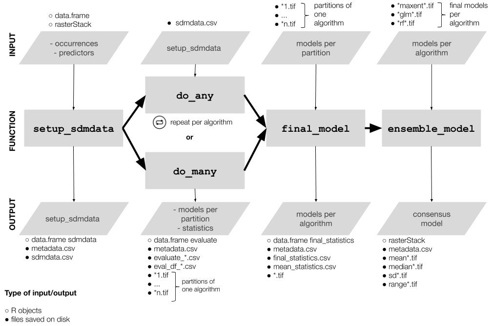 1. Setup: `setup_sdmdata()` prepares and cleans the data, samples the
pseudoabsences, and organizes the experimental design (bootstrap,
crossvalidation or repeated crossvalidation). It creates a metadata
file with details for the current round and a sdmdata file with the
data used for modeling
2. Model fitting and projecting: `do_any()` makes the ENM for one
algorithm and partition; optionally, `do_many()` calls `do_any()` to
fit multiple algorithms
3. Partition joining: `final_model()` joins the partition models into a
model per species per algorithm
4. Ensemble: `ensemble_model()` joins the different models per
algorithm into an ensemble model (algorithmic consensus) using
several methods.
## Folder structure created by this package
**modleR** writes the outputs in the hard disk, according to the
following folder structure:
``` bash
models_dir
├── projection1
│ ├── data_setup
│ ├── partitions
│ ├── final_models
│ └── ensemble_models
└── projection2
├── data_setup
├── partitions
├── final_models
└── ensemble_models
```
- We define a *partition* as the individual modeling round (one training
and test data set and one algorithm)
- We define the *final models* as joining together the partitions and
obtaining **one model per species per algorithm**
- *Ensemble* models join together the results obtained by different
algorithms (Araújo and New 2007)
- When projecting models into the present, the projection folder is
called `present`, other projections will be named after their
environmental variables
- You can set `models_dir` wherever you want in the hard disk, but if
you do not modify the default value, it will create the output under
the working directory (its default value is `./models`, where the
period points to the working directory)
- The *names* of the `final` and `ensemble` folders can be modified, but
**the nested subfolder structure will remain the same**. If you change
`final_models` default value (`"final_model"`) you will need to
include the new value when calling `ensemble_model()`
(`final_dir = "[new name]"`), to indicate the function where to look
for models. This partial flexibility allows for experimenting with
final model and ensemble construction (by runnning final or ensemble
twice in different output folders, for example).
## The example dataset
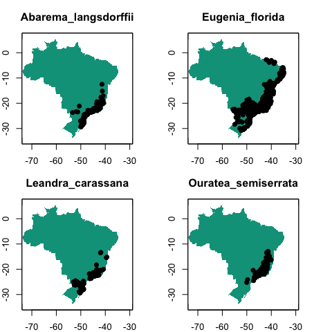
**modleR** comes with example data, a list called `example_occs` with
occurrence data for four species, and predictor variables called
`example_vars`.
``` r
library(modleR)
```
``` r
str(example_occs)
#> List of 4
#> $ Abarema_langsdorffii:'data.frame': 104 obs. of 3 variables:
#> ..$ sp : chr [1:104] "Abarema_langsdorffii" "Abarema_langsdorffii" "Abarema_langsdorffii" "Abarema_langsdorffii" ...
#> ..$ lon: num [1:104] -40.6 -40.7 -41.2 -41.7 -42.5 ...
#> ..$ lat: num [1:104] -19.9 -20 -20.3 -20.5 -20.7 ...
#> $ Eugenia_florida :'data.frame': 341 obs. of 3 variables:
#> ..$ sp : chr [1:341] "Eugenia_florida" "Eugenia_florida" "Eugenia_florida" "Eugenia_florida" ...
#> ..$ lon: num [1:341] -35 -34.9 -34.9 -36.4 -42.1 ...
#> ..$ lat: num [1:341] -6.38 -7.78 -8.1 -10.42 -2.72 ...
#> $ Leandra_carassana :'data.frame': 82 obs. of 3 variables:
#> ..$ sp : chr [1:82] "Leandra_carassana" "Leandra_carassana" "Leandra_carassana" "Leandra_carassana" ...
#> ..$ lon: num [1:82] -39.3 -39.6 -40.7 -41.2 -41.5 ...
#> ..$ lat: num [1:82] -15.2 -15.4 -20 -20.3 -20.4 ...
#> $ Ouratea_semiserrata :'data.frame': 90 obs. of 3 variables:
#> ..$ sp : chr [1:90] "Ouratea_semiserrata" "Ouratea_semiserrata" "Ouratea_semiserrata" "Ouratea_semiserrata" ...
#> ..$ lon: num [1:90] -40 -42.5 -42.4 -42.9 -42.6 ...
#> ..$ lat: num [1:90] -16.4 -20.7 -19.5 -19.6 -19.7 ...
species <- names(example_occs)
species
#> [1] "Abarema_langsdorffii" "Eugenia_florida" "Leandra_carassana"
#> [4] "Ouratea_semiserrata"
```
``` r
library(sp)
par(mfrow = c(2, 2), mar = c(2, 2, 3, 1))
for (i in 1:length(example_occs)) {
plot(!is.na(example_vars[[1]]),
legend = FALSE,
main = species[i],
col = c("white", "#00A08A"))
points(lat ~ lon, data = example_occs[[i]], pch = 19)
}
par(mfrow = c(1, 1))
```
1. Setup: `setup_sdmdata()` prepares and cleans the data, samples the
pseudoabsences, and organizes the experimental design (bootstrap,
crossvalidation or repeated crossvalidation). It creates a metadata
file with details for the current round and a sdmdata file with the
data used for modeling
2. Model fitting and projecting: `do_any()` makes the ENM for one
algorithm and partition; optionally, `do_many()` calls `do_any()` to
fit multiple algorithms
3. Partition joining: `final_model()` joins the partition models into a
model per species per algorithm
4. Ensemble: `ensemble_model()` joins the different models per
algorithm into an ensemble model (algorithmic consensus) using
several methods.
## Folder structure created by this package
**modleR** writes the outputs in the hard disk, according to the
following folder structure:
``` bash
models_dir
├── projection1
│ ├── data_setup
│ ├── partitions
│ ├── final_models
│ └── ensemble_models
└── projection2
├── data_setup
├── partitions
├── final_models
└── ensemble_models
```
- We define a *partition* as the individual modeling round (one training
and test data set and one algorithm)
- We define the *final models* as joining together the partitions and
obtaining **one model per species per algorithm**
- *Ensemble* models join together the results obtained by different
algorithms (Araújo and New 2007)
- When projecting models into the present, the projection folder is
called `present`, other projections will be named after their
environmental variables
- You can set `models_dir` wherever you want in the hard disk, but if
you do not modify the default value, it will create the output under
the working directory (its default value is `./models`, where the
period points to the working directory)
- The *names* of the `final` and `ensemble` folders can be modified, but
**the nested subfolder structure will remain the same**. If you change
`final_models` default value (`"final_model"`) you will need to
include the new value when calling `ensemble_model()`
(`final_dir = "[new name]"`), to indicate the function where to look
for models. This partial flexibility allows for experimenting with
final model and ensemble construction (by runnning final or ensemble
twice in different output folders, for example).
## The example dataset
**modleR** comes with example data, a list called `example_occs` with
occurrence data for four species, and predictor variables called
`example_vars`.
``` r
library(modleR)
```
``` r
str(example_occs)
#> List of 4
#> $ Abarema_langsdorffii:'data.frame': 104 obs. of 3 variables:
#> ..$ sp : chr [1:104] "Abarema_langsdorffii" "Abarema_langsdorffii" "Abarema_langsdorffii" "Abarema_langsdorffii" ...
#> ..$ lon: num [1:104] -40.6 -40.7 -41.2 -41.7 -42.5 ...
#> ..$ lat: num [1:104] -19.9 -20 -20.3 -20.5 -20.7 ...
#> $ Eugenia_florida :'data.frame': 341 obs. of 3 variables:
#> ..$ sp : chr [1:341] "Eugenia_florida" "Eugenia_florida" "Eugenia_florida" "Eugenia_florida" ...
#> ..$ lon: num [1:341] -35 -34.9 -34.9 -36.4 -42.1 ...
#> ..$ lat: num [1:341] -6.38 -7.78 -8.1 -10.42 -2.72 ...
#> $ Leandra_carassana :'data.frame': 82 obs. of 3 variables:
#> ..$ sp : chr [1:82] "Leandra_carassana" "Leandra_carassana" "Leandra_carassana" "Leandra_carassana" ...
#> ..$ lon: num [1:82] -39.3 -39.6 -40.7 -41.2 -41.5 ...
#> ..$ lat: num [1:82] -15.2 -15.4 -20 -20.3 -20.4 ...
#> $ Ouratea_semiserrata :'data.frame': 90 obs. of 3 variables:
#> ..$ sp : chr [1:90] "Ouratea_semiserrata" "Ouratea_semiserrata" "Ouratea_semiserrata" "Ouratea_semiserrata" ...
#> ..$ lon: num [1:90] -40 -42.5 -42.4 -42.9 -42.6 ...
#> ..$ lat: num [1:90] -16.4 -20.7 -19.5 -19.6 -19.7 ...
species <- names(example_occs)
species
#> [1] "Abarema_langsdorffii" "Eugenia_florida" "Leandra_carassana"
#> [4] "Ouratea_semiserrata"
```
``` r
library(sp)
par(mfrow = c(2, 2), mar = c(2, 2, 3, 1))
for (i in 1:length(example_occs)) {
plot(!is.na(example_vars[[1]]),
legend = FALSE,
main = species[i],
col = c("white", "#00A08A"))
points(lat ~ lon, data = example_occs[[i]], pch = 19)
}
par(mfrow = c(1, 1))
```
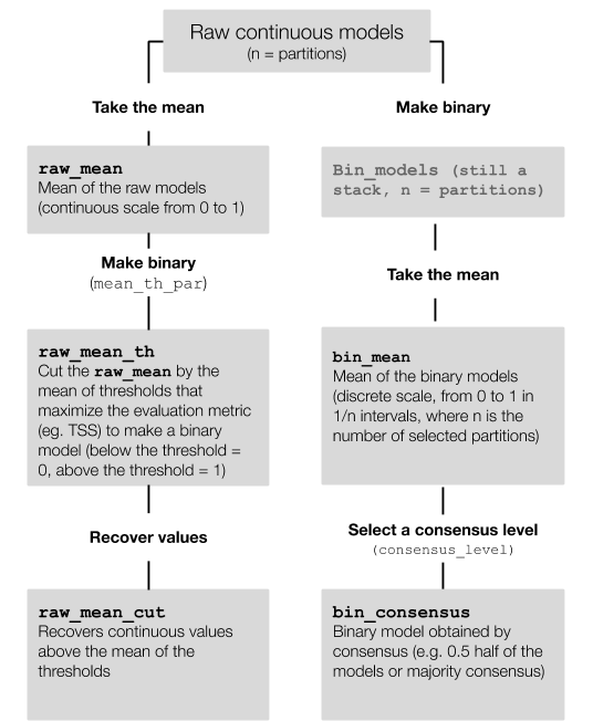 - The partitions that will be joined can be the raw, uncut models, or
the binary models from the previous step, they form a
`raster::rasterStack()` object.
- The means for the raw models can be calculated (`raw_mean`)
- From `raw_mean`, a binary model can be obtained by cutting it by the
mean threshold that maximizes the selected performance metric for each
partition (`bin_th_par`), this is `raw_mean_th`. From this, values
above the threshold can be revovered (`raw_mean_cut`).
- In the case of binary models, since they have already been transformed
into binary, a mean can be calculated (`bin_mean`). This `bin_mean`
reflects the consensus between partitions, and its scale is
categorical.
- From `bin_mean`, a specific consensus level can be chosen (i.e. how
many of the models predict an area, `consensus_level`) and the
resulting binary model can be built (`bin_consensus`). The parameter
`consensus_level` allows to set this level of consensus (defaults to
0.5: majority consensus approach).
- NOTE: The final models can be done using a subset of the algorithms
avaliable on the hard disk, using the parameter `algorithms`. If left
unspecified, all algorithms listed in the `evaluate` files will be
used.
``` r
args(final_model)
#> function (species_name, algorithms = NULL, scale_models = TRUE,
#> consensus_level = 0.5, models_dir = "./models", final_dir = "final_models",
#> proj_dir = "present", which_models = c("raw_mean"), mean_th_par = c("spec_sens"),
#> uncertainty = FALSE, png_final = TRUE, sensitivity = 0.9,
#> ...)
#> NULL
```
``` r
final_model(species_name = species[1],
algorithms = NULL, #if null it will take all the algorithms in disk
models_dir = test_folder,
which_models = c("raw_mean",
"bin_mean",
"bin_consensus"),
consensus_level = 0.5,
uncertainty = TRUE,
overwrite = TRUE)
```
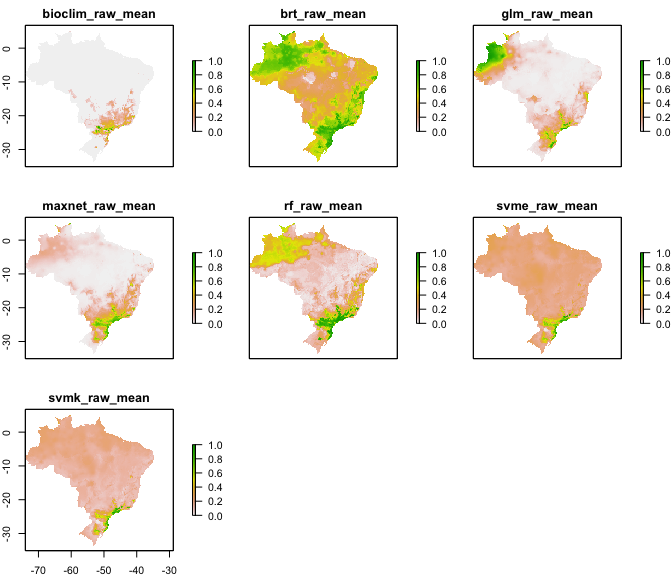
`final_model()` creates a .tif file for each final.model (one per
algorithm) under the specified folder (default: `final_models`)
The `raw_mean` final models for each algorithm are these:
## Algorithmic consensus with `ensemble_model()`
The fourth step of the workflow is joining the models for each algorithm
into a final ensemble model. `ensemble_model()` calculates the mean,
standard deviation, minimum and maximum values of the final models and
saves them under the folder specified by `ensemble_dir`. It can also
create these models by a consensus rule (what proportion of final models
predict a presence in each pixel, 0.5 is a majority rule, 0.3 would be
30% of the models).
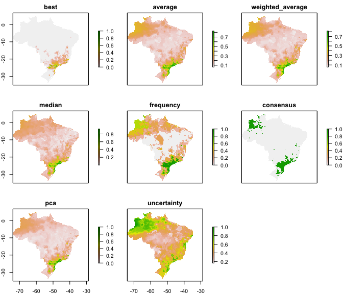
`ensemble_model()` uses a `which_final` parameter -analog to
`which_model` in `final_model()` to specify which final model(s) (Figure
2) should be assembled together (the default is a mean of the raw
continuous models: `which_final = c("raw_mean")`).
``` r
args(ensemble_model)
#> function (species_name, occurrences, lon = "lon", lat = "lat",
#> models_dir = "./models", final_dir = "final_models", ensemble_dir = "ensemble",
#> proj_dir = "present", algorithms = NULL, which_ensemble = c("average"),
#> which_final = c("raw_mean"), performance_metric = "TSSmax",
#> dismo_threshold = "spec_sens", consensus_level = 0.5, png_ensemble = TRUE,
#> write_occs = FALSE, write_map = FALSE, scale_models = TRUE,
#> uncertainty = TRUE, ...)
#> NULL
ens <- ensemble_model(species_name = species[1],
occurrences = occs,
performance_metric = "pROC",
which_ensemble = c("average",
"best",
"frequency",
"weighted_average",
"median",
"pca",
"consensus"),
consensus_level = 0.5,
which_final = "raw_mean",
models_dir = test_folder,
overwrite = TRUE) #argument from writeRaster
#> [1] "Thu Aug 3 11:36:24 2023"
#> [1] "DONE!"
#> [1] "Thu Aug 3 11:36:36 2023"
```
``` r
plot(ens)
```
# Workflows with multiple species
Our `example_occs` dataset has data for four species. An option to do
the several models is to use a `for` loop
``` r
args(do_many)
args(setup_sdmdata)
for (i in 1:length(example_occs)) {
sp <- species[i]
occs <- example_occs[[i]]
setup_sdmdata(species_name = sp,
models_dir = "~/modleR_test/forlooptest",
occurrences = occs,
predictors = example_vars,
buffer_type = "distance",
dist_buf = 4,
write_buffer = TRUE,
clean_dupl = TRUE,
clean_nas = TRUE,
clean_uni = TRUE,
png_sdmdata = TRUE,
n_back = 1000,
partition_type = "bootstrap",
boot_n = 5,
boot_proportion = 0.7
)
}
for (i in 1:length(example_occs)) {
sp <- species[i]
do_many(species_name = sp,
predictors = example_vars,
models_dir = "~/modleR_test/forlooptest",
png_partitions = TRUE,
bioclim = TRUE,
maxnet = FALSE,
rf = TRUE,
svmk = TRUE,
svme = TRUE,
brt = TRUE,
glm = TRUE,
domain = FALSE,
mahal = FALSE,
equalize = TRUE,
write_bin_cut = TRUE)
}
for (i in 1:length(example_occs)) {
sp <- species[i]
final_model(species_name = sp,
consensus_level = 0.5,
models_dir = "~/modleR_test/forlooptest",
which_models = c("raw_mean",
"bin_mean",
"bin_consensus"),
uncertainty = TRUE,
overwrite = TRUE)
}
for (i in 1:length(example_occs)) {
sp <- species[i]
occs <- example_occs[[i]]
ensemble_model(species_name = sp,
occurrences = occs,
which_final = "bin_consensus",
png_ensemble = TRUE,
models_dir = "~/modleR_test/forlooptest")
}
```
Another option is to use the `purrr` package (Henry and Wickham 2017).
``` r
library(purrr)
example_occs %>% purrr::map2(.x = .,
.y = as.list(names(.)),
~ setup_sdmdata(species_name = .y,
occurrences = .x,
partition_type = "bootstrap",
boot_n = 5,
boot_proportion = 0.7,
clean_nas = TRUE,
clean_dupl = TRUE,
clean_uni = TRUE,
buffer_type = "distance",
dist_buf = 4,
predictors = example_vars,
models_dir = "~/modleR_test/temp_purrr",
n_back = 1000))
species %>%
as.list(.) %>%
purrr::map(~ do_many(species_name = .,
predictors = example_vars,
models_dir = "~/modleR_test/temp_purrr",
bioclim = TRUE,
maxnet = FALSE,
rf = TRUE,
svme = TRUE,
svmk = TRUE,
domain = FALSE,
glm = TRUE,
mahal = FALSE,
brt = TRUE,
equalize = TRUE))
```
``` r
species %>%
as.list(.) %>%
purrr::map(~ final_model(species_name = .,
consensus_level = 0.5,
models_dir = "~/modleR_test/temp_purrr",
which_models = c("raw_mean",
"bin_mean",
"bin_consensus"),
overwrite = TRUE))
```
``` r
example_occs %>% purrr::map2(.x = .,
.y = as.list(names(.)),
~ ensemble_model(species_name = .y,
occurrences = .x,
which_final = "raw_mean",
png_ensemble = TRUE,
models_dir = "~/modleR_test/temp_purrr",
overwrite = TRUE))
```
These workflows can also be paralellized by species or species
algorithms
# References
- The partitions that will be joined can be the raw, uncut models, or
the binary models from the previous step, they form a
`raster::rasterStack()` object.
- The means for the raw models can be calculated (`raw_mean`)
- From `raw_mean`, a binary model can be obtained by cutting it by the
mean threshold that maximizes the selected performance metric for each
partition (`bin_th_par`), this is `raw_mean_th`. From this, values
above the threshold can be revovered (`raw_mean_cut`).
- In the case of binary models, since they have already been transformed
into binary, a mean can be calculated (`bin_mean`). This `bin_mean`
reflects the consensus between partitions, and its scale is
categorical.
- From `bin_mean`, a specific consensus level can be chosen (i.e. how
many of the models predict an area, `consensus_level`) and the
resulting binary model can be built (`bin_consensus`). The parameter
`consensus_level` allows to set this level of consensus (defaults to
0.5: majority consensus approach).
- NOTE: The final models can be done using a subset of the algorithms
avaliable on the hard disk, using the parameter `algorithms`. If left
unspecified, all algorithms listed in the `evaluate` files will be
used.
``` r
args(final_model)
#> function (species_name, algorithms = NULL, scale_models = TRUE,
#> consensus_level = 0.5, models_dir = "./models", final_dir = "final_models",
#> proj_dir = "present", which_models = c("raw_mean"), mean_th_par = c("spec_sens"),
#> uncertainty = FALSE, png_final = TRUE, sensitivity = 0.9,
#> ...)
#> NULL
```
``` r
final_model(species_name = species[1],
algorithms = NULL, #if null it will take all the algorithms in disk
models_dir = test_folder,
which_models = c("raw_mean",
"bin_mean",
"bin_consensus"),
consensus_level = 0.5,
uncertainty = TRUE,
overwrite = TRUE)
```
`final_model()` creates a .tif file for each final.model (one per
algorithm) under the specified folder (default: `final_models`)
The `raw_mean` final models for each algorithm are these:

## Algorithmic consensus with `ensemble_model()`
The fourth step of the workflow is joining the models for each algorithm
into a final ensemble model. `ensemble_model()` calculates the mean,
standard deviation, minimum and maximum values of the final models and
saves them under the folder specified by `ensemble_dir`. It can also
create these models by a consensus rule (what proportion of final models
predict a presence in each pixel, 0.5 is a majority rule, 0.3 would be
30% of the models).
`ensemble_model()` uses a `which_final` parameter -analog to
`which_model` in `final_model()` to specify which final model(s) (Figure
2) should be assembled together (the default is a mean of the raw
continuous models: `which_final = c("raw_mean")`).
``` r
args(ensemble_model)
#> function (species_name, occurrences, lon = "lon", lat = "lat",
#> models_dir = "./models", final_dir = "final_models", ensemble_dir = "ensemble",
#> proj_dir = "present", algorithms = NULL, which_ensemble = c("average"),
#> which_final = c("raw_mean"), performance_metric = "TSSmax",
#> dismo_threshold = "spec_sens", consensus_level = 0.5, png_ensemble = TRUE,
#> write_occs = FALSE, write_map = FALSE, scale_models = TRUE,
#> uncertainty = TRUE, ...)
#> NULL
ens <- ensemble_model(species_name = species[1],
occurrences = occs,
performance_metric = "pROC",
which_ensemble = c("average",
"best",
"frequency",
"weighted_average",
"median",
"pca",
"consensus"),
consensus_level = 0.5,
which_final = "raw_mean",
models_dir = test_folder,
overwrite = TRUE) #argument from writeRaster
#> [1] "Thu Aug 3 11:36:24 2023"
#> [1] "DONE!"
#> [1] "Thu Aug 3 11:36:36 2023"
```
``` r
plot(ens)
```

# Workflows with multiple species
Our `example_occs` dataset has data for four species. An option to do
the several models is to use a `for` loop
``` r
args(do_many)
args(setup_sdmdata)
for (i in 1:length(example_occs)) {
sp <- species[i]
occs <- example_occs[[i]]
setup_sdmdata(species_name = sp,
models_dir = "~/modleR_test/forlooptest",
occurrences = occs,
predictors = example_vars,
buffer_type = "distance",
dist_buf = 4,
write_buffer = TRUE,
clean_dupl = TRUE,
clean_nas = TRUE,
clean_uni = TRUE,
png_sdmdata = TRUE,
n_back = 1000,
partition_type = "bootstrap",
boot_n = 5,
boot_proportion = 0.7
)
}
for (i in 1:length(example_occs)) {
sp <- species[i]
do_many(species_name = sp,
predictors = example_vars,
models_dir = "~/modleR_test/forlooptest",
png_partitions = TRUE,
bioclim = TRUE,
maxnet = FALSE,
rf = TRUE,
svmk = TRUE,
svme = TRUE,
brt = TRUE,
glm = TRUE,
domain = FALSE,
mahal = FALSE,
equalize = TRUE,
write_bin_cut = TRUE)
}
for (i in 1:length(example_occs)) {
sp <- species[i]
final_model(species_name = sp,
consensus_level = 0.5,
models_dir = "~/modleR_test/forlooptest",
which_models = c("raw_mean",
"bin_mean",
"bin_consensus"),
uncertainty = TRUE,
overwrite = TRUE)
}
for (i in 1:length(example_occs)) {
sp <- species[i]
occs <- example_occs[[i]]
ensemble_model(species_name = sp,
occurrences = occs,
which_final = "bin_consensus",
png_ensemble = TRUE,
models_dir = "~/modleR_test/forlooptest")
}
```
Another option is to use the `purrr` package (Henry and Wickham 2017).
``` r
library(purrr)
example_occs %>% purrr::map2(.x = .,
.y = as.list(names(.)),
~ setup_sdmdata(species_name = .y,
occurrences = .x,
partition_type = "bootstrap",
boot_n = 5,
boot_proportion = 0.7,
clean_nas = TRUE,
clean_dupl = TRUE,
clean_uni = TRUE,
buffer_type = "distance",
dist_buf = 4,
predictors = example_vars,
models_dir = "~/modleR_test/temp_purrr",
n_back = 1000))
species %>%
as.list(.) %>%
purrr::map(~ do_many(species_name = .,
predictors = example_vars,
models_dir = "~/modleR_test/temp_purrr",
bioclim = TRUE,
maxnet = FALSE,
rf = TRUE,
svme = TRUE,
svmk = TRUE,
domain = FALSE,
glm = TRUE,
mahal = FALSE,
brt = TRUE,
equalize = TRUE))
```
``` r
species %>%
as.list(.) %>%
purrr::map(~ final_model(species_name = .,
consensus_level = 0.5,
models_dir = "~/modleR_test/temp_purrr",
which_models = c("raw_mean",
"bin_mean",
"bin_consensus"),
overwrite = TRUE))
```
``` r
example_occs %>% purrr::map2(.x = .,
.y = as.list(names(.)),
~ ensemble_model(species_name = .y,
occurrences = .x,
which_final = "raw_mean",
png_ensemble = TRUE,
models_dir = "~/modleR_test/temp_purrr",
overwrite = TRUE))
```
These workflows can also be paralellized by species or species
algorithms
# References
Araújo, M, and M New. 2007. “Ensemble Forecasting of Species
Distributions.” *Trends in Ecology & Evolution* 22 (1): 42–47.
.
Elith, J., J. R. Leathwick, and T. Hastie. 2009. “A Working Guide to
Boosted Regression Trees.” *Journal of Animal Ecology* 77 (4): 802–13.
.
Hastie, Trevor, Robert Tibshirani, and Jerome Friedman. 2001. *The
Elements of Statistical Learning: Data Mining, Inference, and
Prediction*. Springer Heidelberg.
Henry, Lionel, and Hadley Wickham. 2017. “Purrr: Functional Programming
Tools. R Package Version 0.2.4.”
Hijmans, Robert J., Steven Phillips, John Leathwick, and Jane Elith.
2017. “Dismo: Species Distribution Modeling. R Package Version 1.1-4.”
Karatzoglou, Alexandros, Alex Smola, Kurt Hornik, and Achim Zeileis.
2004. “Kernlab - An S4 Package for Kernel Methods in R.” *Journal of
Statistical Software* 11 (9): 1–20.
Liaw, Andy, and Matthew Wiener. 2002. “Classification and Regression by
randomForest.” *R News* 2 (3): 18–22.
Meyer, David, Evgenia Dimitriadou, Kurt Hornik, Andreas Weingessel, and
Friedrich Leisch. 2017. “E1071: Misc Functions of the Department of
Statistics, Probability Theory Group (Formerly: E1071), TU Wien.”