With linear models we can answer questions such as:
is there a relationship between exposure and outcome, e.g. body weight and plasma volume?
how strong is the relationship between the two variables?
what will be a predicted value of the outcome given a new set of exposure values?
how accurately can we predict outcome?
which variables are associated with the response, e.g. is it body weight and height that can explain the plasma volume or is it just the body weight?
Statistical vs. deterministic relationship
Relationships in probability and statistics can generally be one of three things:
deterministic
random
statistical
Statistical vs. deterministic relationship
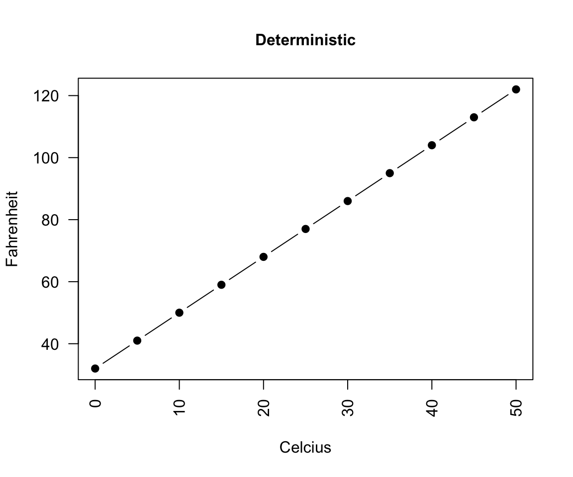
deterministic
A deterministic relationship involves an exact relationship between two variables, for instance Fahrenheit and Celsius degrees is defined by an equation \(Fahrenheit=\frac{9}{5}\cdot Celcius+32\)
Statistical vs. deterministic relationship
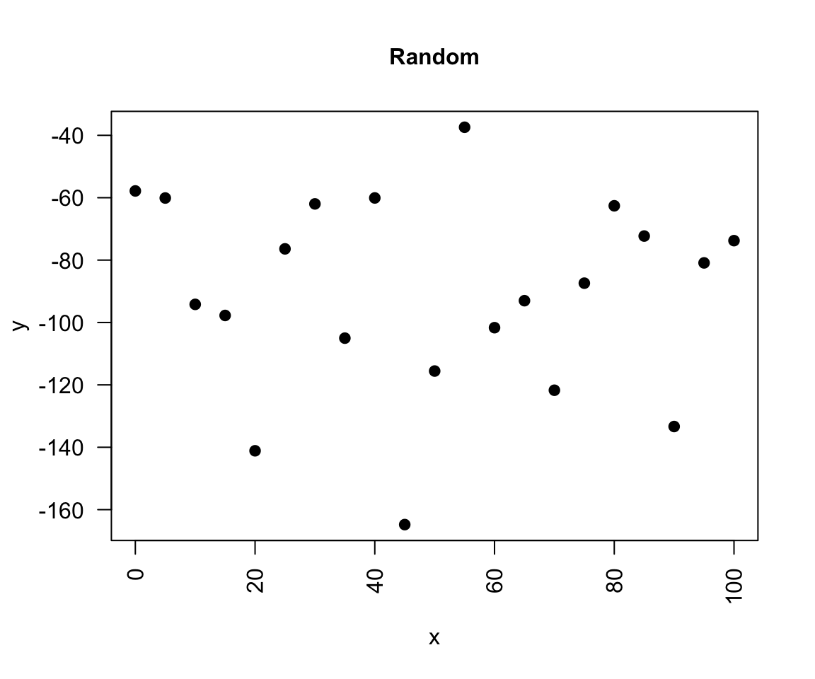
random
There is no relationship between variables in the random relationship, e.g. number of plants Olga buys and time of the year as Olga buys plants whenever she feels like it throughout the entire year
Statistical vs. deterministic relationship
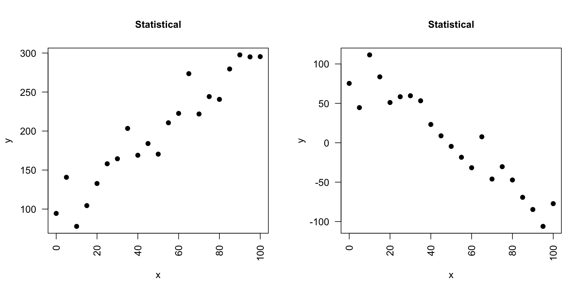
statistical relationship
A statistical relationship is a mixture of deterministic and random relationship, e.g. the savings that Olga has left in the bank account depend on Olga’s monthly salary income (deterministic part) and the money spent on buying plants (random part)
What linear models are and are not
A linear model is one in which the parameters appear linearly in the deterministic part of the model
e.g. simple linear regression through the origin is a simple linear model of the form \[Y_i = \beta x + \epsilon\] often used to express a relationship of one numerical variable to another, e.g. the calories burnt and the kilometers cycled
linear models can become quite advanced by including many variables, e.g. the calories burnt could be a function of the kilometers cycled, road incline and status of a bike
or the transformation of the variables, e.g. a function of kilometers cycled squared
and an example on a non-linear model where parameter \(\beta\) appears in the exponent of \(x_i\)
\(Y_i = \alpha + x_i^\beta + \epsilon\)
What linear models are and are not
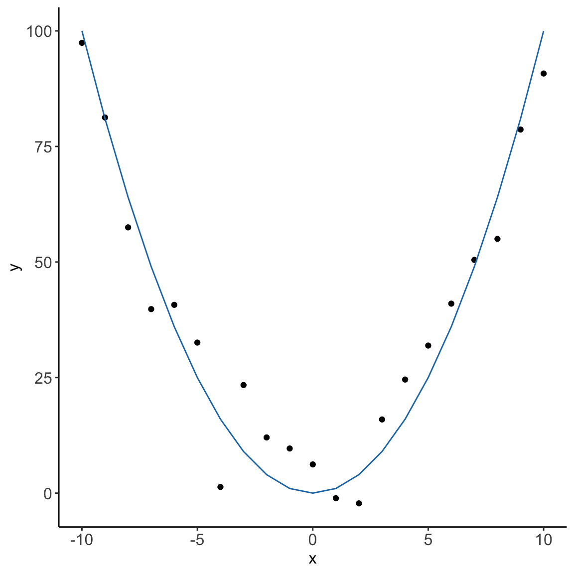
What about this one?
Yes, it’s an example of a linear model: \(y_i = x_i^2 + \epsilon_i\) showing that linear models can capture more than a straight line relationship
Terminology
There are many terms and notations used interchangeably
\(y\) is being called:
response
outcome
dependent variable
\(x\) is being called:
exposure
explanatory variable
dependent variable
predictor
covariate
Simple linear regression
It is used to check the association between the numerical outcome and one numerical explanatory variable
In practice, we are finding the best-fitting straight line to describe the relationship between the outcome and exposure
Simple linear regression
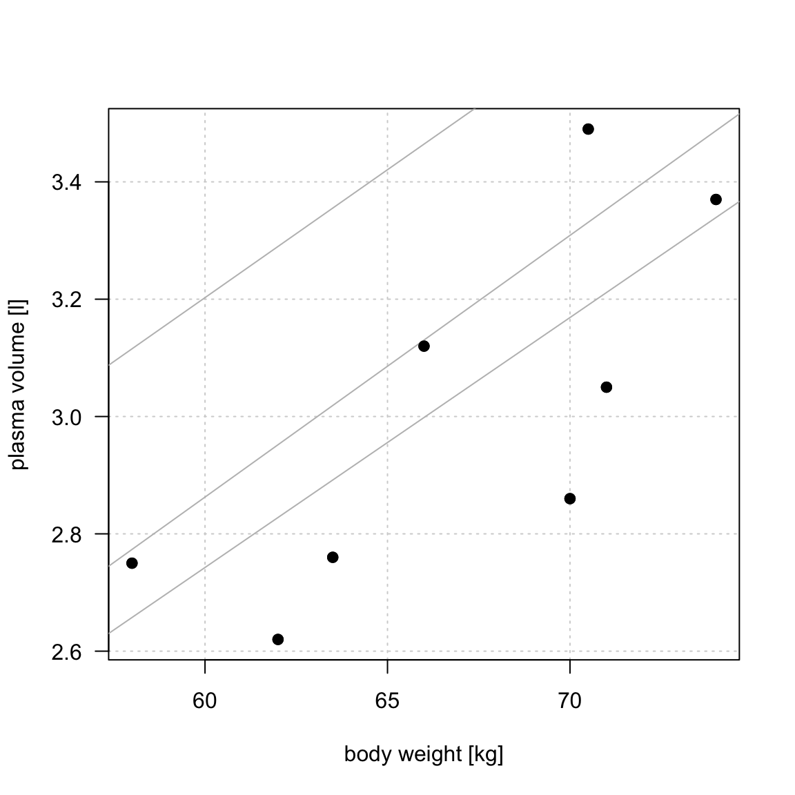
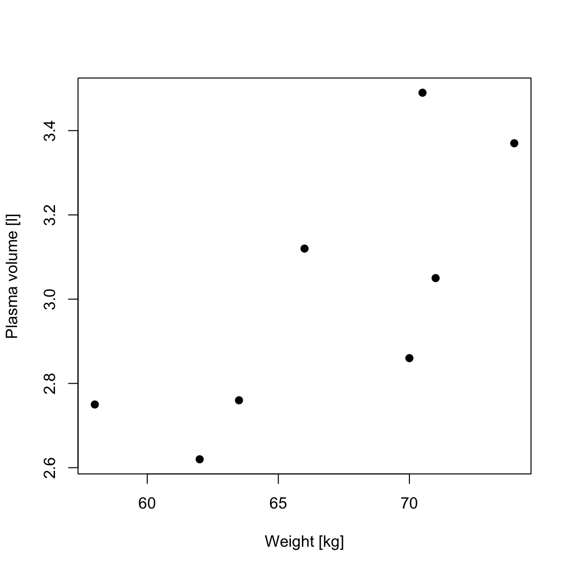
Example 1 (Weight and plasma volume) Let’s look at the example data containing body weight (kg) and plasma volume (liters) for eight healthy men to see what the best-fitting straight line is.
Figure 1: Scatter plot of the data shows that high plasma volume tends to be associated with high weight and vice verca.
Simple linear regression
Simple linear regression
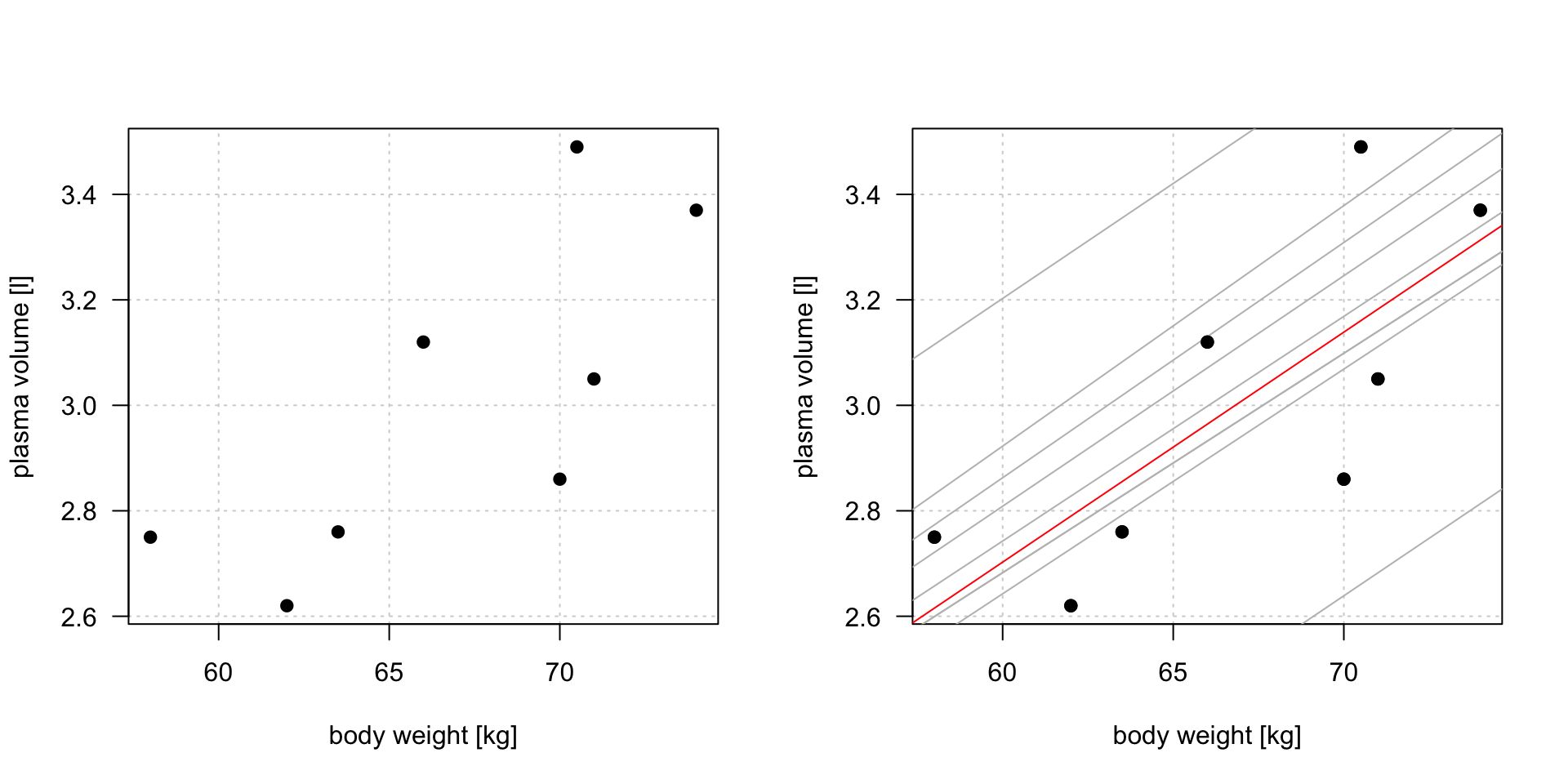
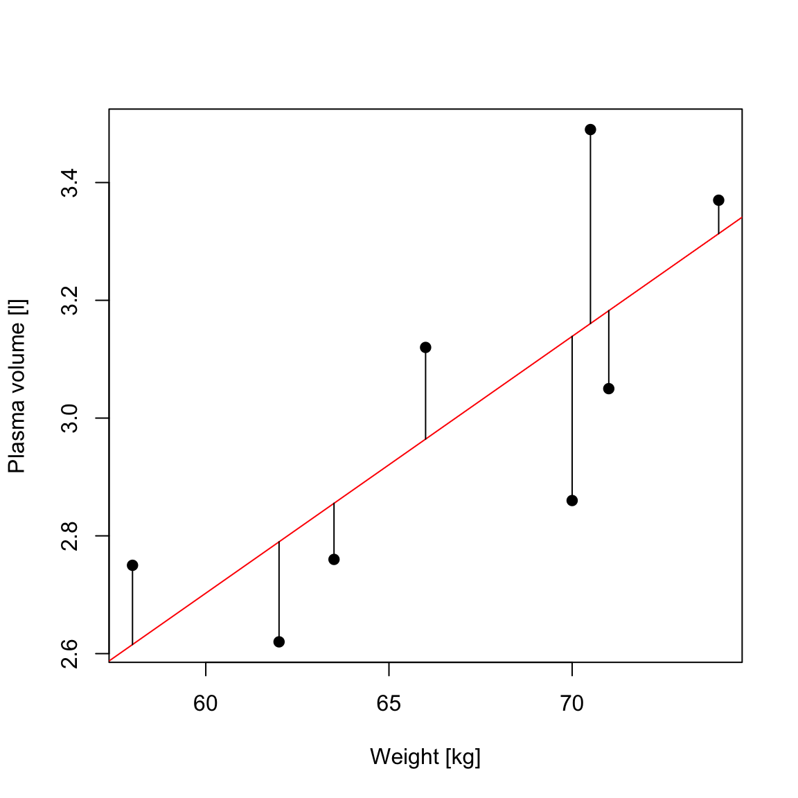
Figure 2: Scatter plot of the data shows that high plasma volume tends to be associated with high weight and vice verca. Linear regression gives the equation of the straight line (red) that best describes how the outcome changes (increase or decreases) with a change of exposure variable
The equation for the red line is: \[Y_i=0.086 + 0.044 \cdot x_i \quad for \;i = 1 \dots 8\]
and in general: \[Y_i=\alpha + \beta \cdot x_i \quad for \; i = 1 \dots n \qquad(1)\]
Simple linear regression
In other words, by finding the best-fitting straight line we are building a statistical model to represent the relationship between plasma volume (\(Y\)) and explanatory body weight variable (\(x\))
\(y\): is called: response, outcome, dependent variable
\(\alpha\) and \(\beta\) are model coefficients
and \(\epsilon_i\) is an error terms
Least squares
in the above “body weight - plasma volume” example, the values of \(\alpha\) and \(\beta\) have just appeared
in practice, \(\alpha\) and \(\beta\) values are unknown and we use data to estimate these coefficients, noting the estimates with a hat, \(\hat{\alpha}\) and \(\hat{\beta}\)
least squares is one of the methods of parameters estimation, i.e. finding \(\hat{\alpha}\) and \(\hat{\beta}\)
Least squares
minimizing RSS
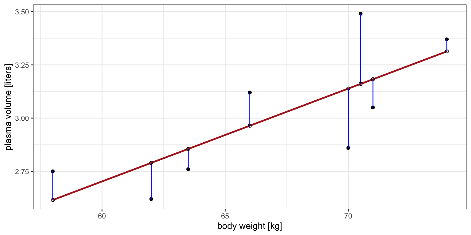
Figure 3: Scatter plot of the data shows that high plasma volume tends to be associated with high weight and vice versa. Linear regression gives the equation of the straight line (red) that best describes how the outcome changes with a change of exposure variable. Blue lines represent error terms, the vertical distances to the regression line
Let \(\hat{y_i}=\hat{\alpha} + \hat{\beta}x_i\) be the prediction \(y_i\) based on the \(i\)-th value of \(x\):
Then \(\epsilon_i = y_i - \hat{y_i}\) represents the \(i\)-th residual, i.e. the difference between the \(i\)-th observed response value and the \(i\)-th response value that is predicted by the linear model
RSS, the residual sum of squares is defined as: \[RSS = \epsilon_1^2 + \epsilon_2^2 + \dots + \epsilon_n^2\] or equivalently as: \[RSS=(y_1-\hat{\alpha}-\hat{\beta}x_1)^2+(y_2-\hat{\alpha}-\hat{\beta}x_2)^2+...+(y_n-\hat{\alpha}-\hat{\beta}x_n)^2\]
the least squares approach chooses \(\hat{\alpha}\) and \(\hat{\beta}\)to minimize the RSS. With some calculus, we get Theorem 1
Least squares
Theorem 1 (Least squares estimates for a simple linear regression) \[\hat{\beta} = \frac{S_{xy}}{S_{xx}}\]\[\hat{\alpha} = \bar{y}-\frac{S_{xy}}{S_{xx}}\cdot \bar{x}\]
where:
\(\bar{x}\): mean value of \(x\)
\(\bar{y}\): mean value of \(y\)
\(S_{xx}\): sum of squares of \(X\) defined as \(S_{xx} = \displaystyle \sum_{i=1}^{n}(x_i-\bar{x})^2\)
\(S_{yy}\): sum of squares of \(Y\) defined as \(S_{yy} = \displaystyle \sum_{i=1}^{n}(y_i-\bar{y})^2\)
\(S_{xy}\): sum of products of \(X\) and \(Y\) defined as \(S_{xy} = \displaystyle \sum_{i=1}^{n}(x_i-\bar{x})(y_i-\bar{y})\)
Least squares
We can further re-write the above sum of squares to obtain
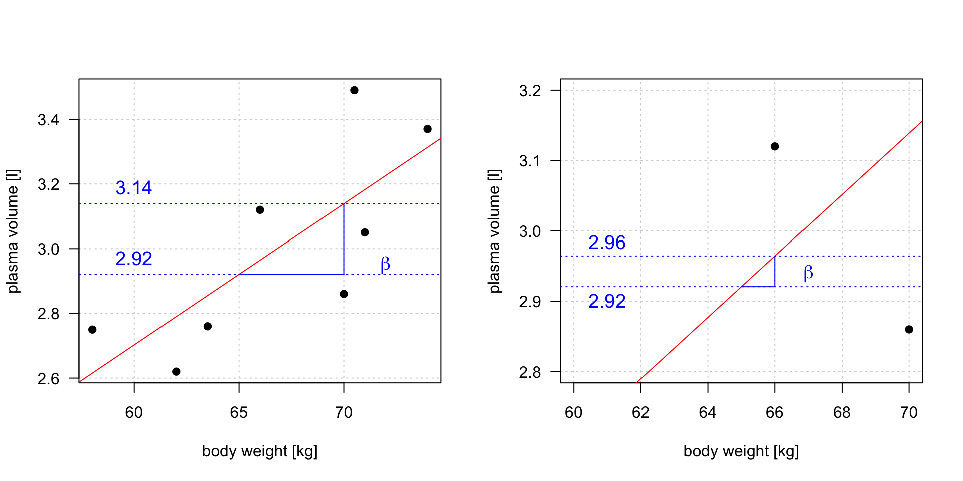
Linear regression gives us estimates of model coefficient \(Y_i = \alpha + \beta x_i + \epsilon_i\)
Increasing weight by 5 kg corresponds to \(3.14 - 2.92 = 0.22\) increase in plasma volume. Increasing weight by 1 kg corresponds \(2.96 - 2.92 = 0.04\) increase in plasma volume
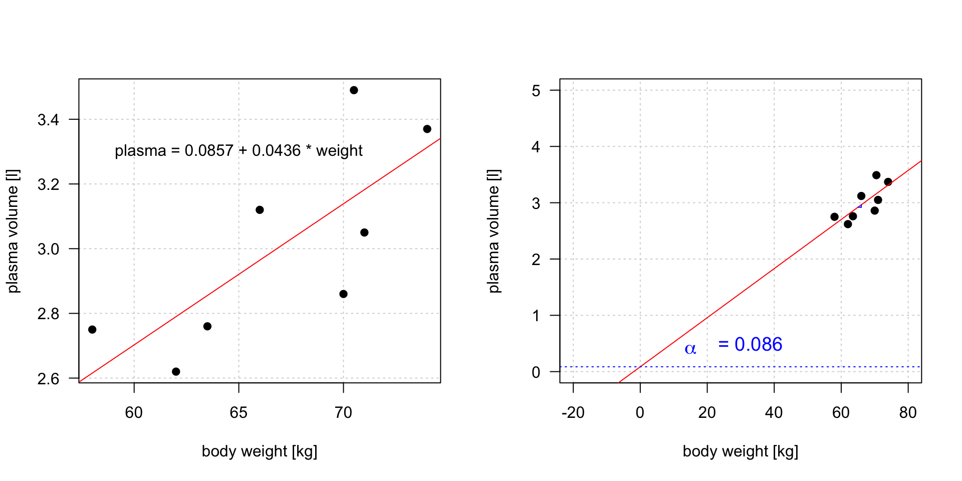
Intercept
\(plasma = 0.0857 + 0.0436 * weight\)
Linear regression gives us estimates of model coefficient \(Y_i = \alpha + \beta x_i + \epsilon_i\)
Intercept value corresponds to expected outcome when the explanatory variable value equals to zero. It is not always meaningful
Hypothesis testing
Is there a relationship between the response and the predictor?
the calculated \(\hat{\alpha}\) and \(\hat{\beta}\) are estimates of the population values of the intercept and slope and are therefore subject to sampling variation
their precision is measured by their estimated standard errors, e.s.e(\(\hat{\alpha}\)) and e.s.e(\(\hat{\beta}\))
these estimated standard errors are used in hypothesis testing and in constructing confidence and prediction intervals
Hypothesis testing
The most common hypothesis test involves testing the null hypothesis of:
\(H_0:\) There is no relationship between \(X\) and \(Y\)
versus the alternative hypothesis\(H_a:\) there is some relationship between \(X\) and \(Y\)
Mathematically, this corresponds to testing:
\(H_0: \beta=0\)
versus \(H_a: \beta\neq0\)
since if \(\beta=0\) then the model \(Y_i=\alpha+\beta x_i + \epsilon_i\) reduces to \(Y=\alpha + \epsilon_i\)
Under the null hypothesis\(H_0: \beta = 0\)
\(n\) is number of observations
\(p\) is number of model parameters
\(\frac{\hat{\beta}-\beta}{e.s.e(\hat{\beta})}\) is the ratio of the departure of the estimated value of a parameter, \(\hat\beta\), from its hypothesized value, \(\beta\), to its standard error, called t-statistics
the t-statistics follows Student’s t distribution with \(n-p\) degrees of freedom
Hypothesis testing
Example 3 (Hypothesis testing) Let’s look again at our example data. This time we will not only fit the linear regression model but also look a bit more closely at the R summary of the model
Call:
lm(formula = plasma ~ weight)

Residuals:
     Min       1Q   Median       3Q      Max
-0.27880 -0.14178 -0.01928  0.13986  0.32939

Coefficients:
            Estimate Std. Error t value Pr(>|t|)
(Intercept)  0.08572    1.02400   0.084   0.9360
weight       0.04362    0.01527   2.857   0.0289 *
---
Signif. codes:  0 '***' 0.001 '**' 0.01 '*' 0.05 '.' 0.1 ' ' 1

Residual standard error: 0.2188 on 6 degrees of freedom
Multiple R-squared:  0.5763,    Adjusted R-squared:  0.5057
F-statistic:  8.16 on 1 and 6 DF,  p-value: 0.02893
Under Estimate we see estimates of our model coefficients, \(\hat{\alpha}\) (intercept) and \(\hat{\beta}\) (slope, here weight), followed by their estimated standard errors, Std. Errors
If we were to test if there is an association between weight and plasma volume we would write under the null hypothesis \(H_0: \beta = 0\)\[\frac{\hat{\beta}-\beta}{e.s.e(\hat{\beta})} = \frac{0.04362-0}{0.01527} = 2.856582\]
and we would comparet-statistics to Student's t distribution with \(n-p = 8 - 2 = 6\) degrees of freedom (as we have 8 observations and two model parameters, \(\alpha\) and \(\beta\))
we can use Student’s t distribution table or R code to obtain the associated P-value
2*pt(2.856582, df=6, lower=F)
[1] 0.02893095
here the observed t-statistics is large and therefore yields a small P-value, meaning that there is sufficient evidence to reject null hypothesis in favor of the alternative and conclude that there is a significant association between weight and plasma volume
Vector-matrix notations
While in simple linear regression it is feasible to arrive at the parameters estimates using calculus in more realistic settings of multiple regression, with more than one explanatory variable in the model, it is more efficient to use vectors and matrices to define the regression model.
Let’s rewrite our simple linear regression model \(Y_i = \alpha + \beta_i + \epsilon_i \quad i=1,\dots n\)into vector-matrix notation in 6 steps.
Step 1. First we rename our \(\alpha\) to \(\beta_0\) and \(\beta\) to \(\beta_1\) as it is easier to keep tracking the number of model parameters this way
Step 2. Then we notice that we actually have \(n\) equations such as:
Step 3. We group all \(Y_i\) and \(\epsilon_i\) into column vectors: \(\mathbf{Y}=\begin{bmatrix} y_1 \\ y_2 \\ \vdots \\ y_{n} \end{bmatrix}\) and \(\boldsymbol\epsilon=\begin{bmatrix} \epsilon_1 \\ \epsilon_2 \\ \vdots \\ \epsilon_{n} \end{bmatrix}\)
Step 4. We stack two parameters \(\beta_0\) and \(\beta_1\) into another column vector:\[\boldsymbol\beta=\begin{bmatrix}
\beta_0 \\
\beta_1
\end{bmatrix}\]
Step 5. We append a vector of ones with the single predictor for each \(i\) and create a matrix with two columns called design matrix\[\mathbf{X}=\begin{bmatrix}
1 & x_1 \\
1 & x_2 \\
\vdots & \vdots \\
1 & x_{n}
\end{bmatrix}\]
Step 6. We write our linear model in a vector-matrix notations as: \[\mathbf{Y} = \mathbf{X}\boldsymbol\beta + \boldsymbol\epsilon\]
Vector-matrix notations
Definition 1 (vector matrix form of the linear model) The vector-matrix representation of a linear model with \(p-1\) predictors can be written as \[\mathbf{Y} = \mathbf{X}\boldsymbol\beta + \boldsymbol\epsilon\]
where:
\(\mathbf{Y}\) is \(n \times1\) vector of observations
\(\mathbf{X}\) is \(n \times p\)design matrix
\(\boldsymbol\beta\) is \(p \times1\) vector of parameters
\(\boldsymbol\epsilon\) is \(n \times1\) vector of vector of random errors, indepedent and identically distributed (i.i.d) N(0, \(\sigma^2\))
In full, the above vectors and matrix have the form:
Theorem 2 (Least squares in vector-matrix notation) The least squares estimates for a linear regression of the form: \[\mathbf{Y} = \mathbf{X}\boldsymbol\beta + \boldsymbol\epsilon\]
is given by: \[\hat{\mathbf{\beta}}= (\mathbf{X}^T\mathbf{X})^{-1}\mathbf{X}^T\mathbf{Y}\]
Vector-matrix notations
Example 4 (vector-matrix-notation) Following the above definition we can write the “weight - plasma volume model” as: \[\mathbf{Y} = \mathbf{X}\boldsymbol\beta + \boldsymbol\epsilon\] where:
and we can estimate model parameters using \(\hat{\mathbf{\beta}}= (\mathbf{X}^T\mathbf{X})^{-1}\mathbf{X}^T\mathbf{Y}\).
Vector-matrix notations
Live demo
Estimating model parameters using \(\hat{\mathbf{\beta}}= (\mathbf{X}^T\mathbf{X})^{-1}\mathbf{X}^T\mathbf{Y}\).
n <-length(plasma) # no. of observationY <-as.matrix(plasma, ncol=1)X <-cbind(rep(1, length=n), weight)X <-as.matrix(X)# print Y and X to double-check that the format is according to the definitionprint(Y)print(X)# least squares estimate# solve() finds inverse of matrixbeta.hat <-solve(t(X)%*%X)%*%t(X)%*%Yprint(beta.hat)
             [,1]
       0.08572428
weight 0.04361534
Thank you for listening
Any questions?
Model diagnostics
Assessing model fit and validity
Assessing model fit
earlier we learned how to estimate parameters in a liner model using least squares
now we will consider how to assess the goodness of fit of a model
we do that by calculating the amount of variability in the response that is explained by the model
\(R^2\): summary of the fitted model
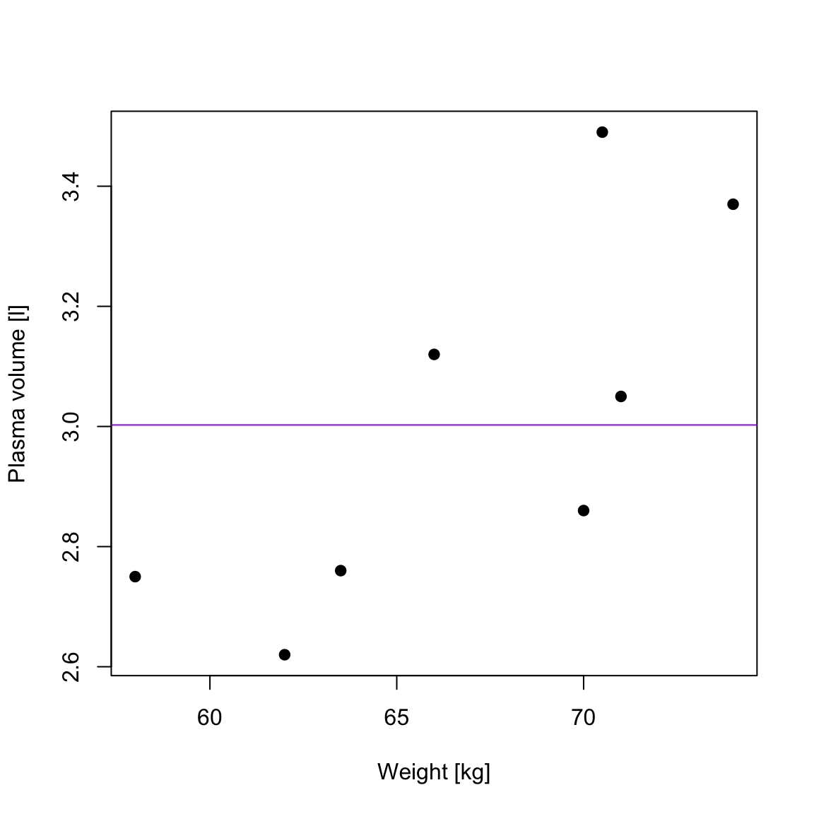
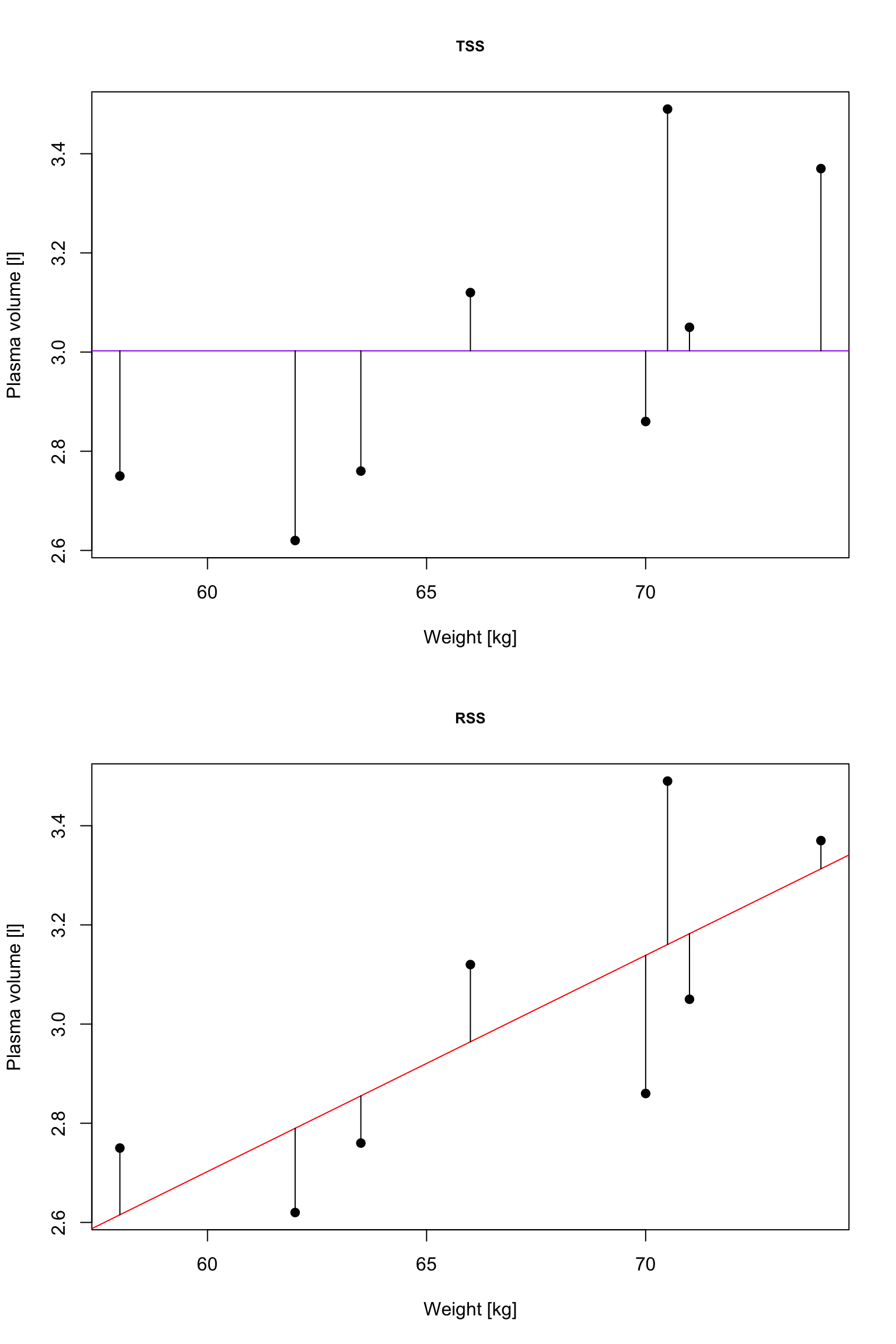
TSS
\(R^2\): summary of the fitted model
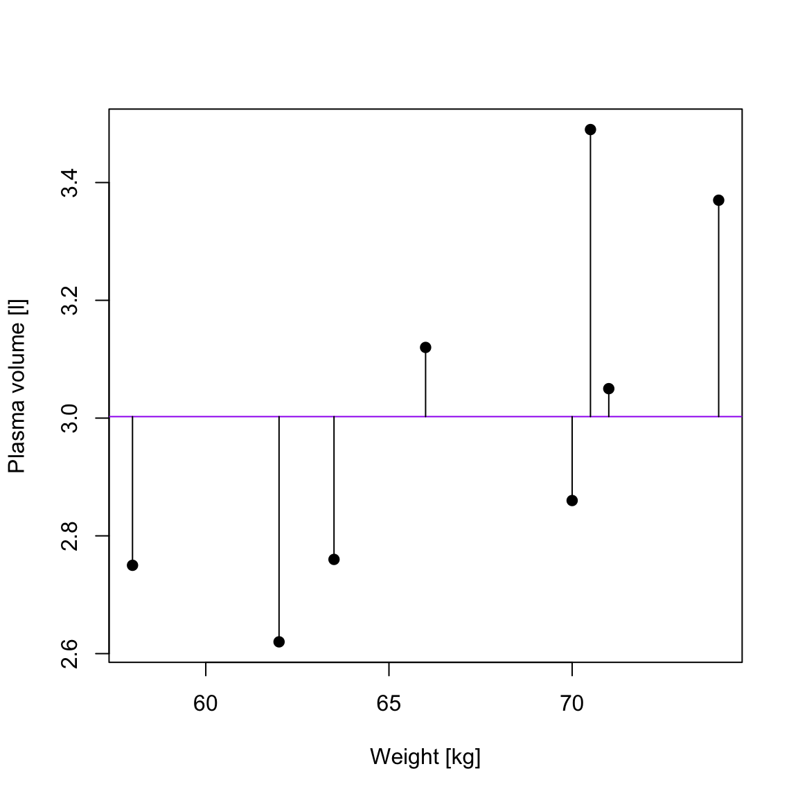
RSS
\(R^2\): summary of the fitted model
TSS, denoted Total corrected sum-of-squares is the residual sum-of-squares for Model 0 \[S(\hat{\beta_0}) = TSS = \sum_{i=1}^{n}(y_i - \bar{y})^2 = S_{yy}\] corresponding the to the sum of squared distances to the purple line
and corresponds to the squared distances between the observed values \(y_i, \dots,y_n\) to fitted values \(\hat{y_1}, \dots \hat{y_n}\), i.e. distances to the red fitted line
\(R^2\): summary of the fitted model
Definition 2 (\(R^2\)) A simple but useful measure of model fit is given by \[R^2 = 1 - \frac{RSS}{TSS}\] where:
RSS is the residual sum-of-squares for Model 1, the fitted model of interest
TSS is the sum of squares of the null model
\(R^2\): summary of the fitted model
\(R^2\) quantifies how much of a drop in the residual sum-of-squares is accounted for by fitting the proposed model
\(R^2\) is also referred as coefficient of determination
It is expressed on a scale, as a proportion (between 0 and 1) of the total variation in the data
Values of \(R^2\) approaching 1 indicate the model to be a good fit
Values of \(R^2\) less than 0.5 suggest that the model gives rather a poor fit to the data
\(R^2\) and correlation coefficient
Theorem 3 (\(R^2\)) In the case of simple linear regression:
Model 1: \(Y_i = \beta_0 + \beta_1x + \epsilon_i\)
\[R^2 = r^2\]
where:
\(R^2\) is the coefficient of determination
\(r^2\) is the sample correlation coefficient
\(R^2(adj)\)
in the case of multiple linear regression, where there is more than one explanatory variable in the model
we are using the adjusted version of \(R^2\) to assess the model fit as the number of explanatory variables increase, \(R^2\) also increases
\(R^2(adj)\) takes this into account, i.e. adjusts for the fact that there is more than one explanatory variable in the model
Theorem 4 (\(R^2(adj)\)) For any multiple linear regression
\[Y_i = \beta_0 + \beta_1x_{1i} + \dots + \beta_{p-1}x_{(p-1)i} + \epsilon_i\]\(R^2(adj)\) is defined as \[R^2(adj) = 1-\frac{\frac{RSS}{n-p-1}}{\frac{TSS}{n-1}}\] where
\(p\) is the number of independent predictors, i.e. the number of variables in the model, excluding the constant
\(R^2(adj)\) can also be calculated from \(R^2\):
\[R^2(adj) = 1 - (1-R^2)\frac{n-1}{n-p-1}\]
\(R^2\)
Live demo
htwtgen <-read.csv("data/lm/heights_weights_gender.csv")head(htwtgen)attach(htwtgen)## Simple linear regressionmodel.simple <-lm(Height ~ Weight, data=htwtgen)# TSSTSS <-sum((Height -mean(Height))^2)# RSS# residuals are returned in the model type names(model.simple)RSS <-sum((model.simple$residuals)^2)R2 <-1- (RSS/TSS)print(R2)print(summary(model.simple))
up until now we were fitting models and discussed how to assess the model fit
before making use of a fitted model for explanation or prediction, it is wise to check that the model provides an adequate description of the data
informally we have been using box plots and scatter plots to look at the data
there are however formal definitions of the assumptions
The assumptions of a linear model
Linearity:
The relationship between \(X\) and \(Y\) is linear
Independence of errors
\(Y\) is independent of errors, there is no relationship between the residuals and \(Y\)
Normality of errors
The residuals must be approximately normally distributed
Equal variances
The variance of the residuals is the same for all values of \(X\)
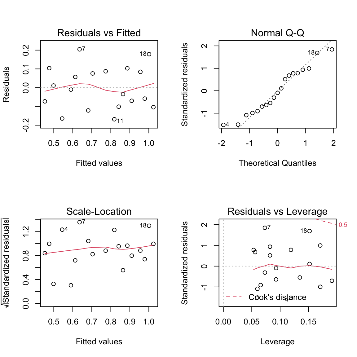
Checking assumptions
Residuals, \(\hat{\epsilon_i} = y_i - \hat{y_i}\) are the main ingredient to check model assumptions.
Selecting best model
Now we have learnt what linear models are, how to find estimates and interpret the model coefficients. And we now know how to assess the model.
Exercise 1 (Features selection)
Imagine you have gene expression measurements for 12 genes and you want to build the best linear regression model to study protein levels of protein P. You can use any combinations of genes. How would you go about building the model and how would you decide which model is the best one?
Selecting best model
As a rule of thumb, we want a model that fits the data best and is as simple as possible, meaning it contains only relevant predictors.
In practice, this means, that for smaller data sets, e.g. with up to 10 predictors, one works with manually trying different models, including different subsets of predictors, interactions terms and/or their transformations.
When the number of predictors is large, one can try automated approaches of feature selection like forward selection or stepwise regression (see exercises for demo).
On Friday, we use regularization techniques that allow including all parameters in the model but constraining (regularizing) coefficient estimates towards zero for the less relevant predictors, preventing building complex models and thus overfitting.