{
"cells": [
{
"cell_type": "markdown",
"metadata": {},
"source": [
"# Focusing Properties of a Binary-Phase Zone Plate\n",
"\n",
"It is also possible to compute a [near-to-far field transformation](https://meep.readthedocs.io/en/latest/Python_User_Interface/#near-to-far-field-spectra) in cylindrical coordinates. This is demonstrated in this example for a binary-phase [zone plate](https://en.wikipedia.org/wiki/Zone_plate) which is a rotationally-symmetric diffractive lens used to focus a normally-incident planewave to a single spot.\n",
"\n",
"Using [scalar theory](http://zoneplate.lbl.gov/theory), the radius of the $n$th zone can be computed as:\n",
"\n",
"\n",
"$$ r_n^2 = n\\lambda (f+\\frac{n\\lambda}{4})$$\n",
"\n",
"\n",
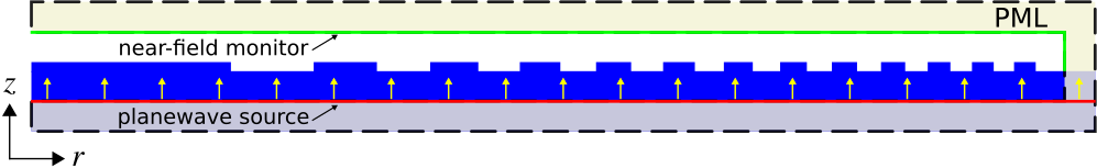
"where $n$ is the zone index (1,2,3,...,$N$), $f$ is the focal length, and $\\lambda$ is the operating wavelength. The main design variable is the number of zones $N$. The design specifications of the zone plate are similar to the binary-phase grating in [Tutorial/Mode Decomposition/Diffraction Spectrum of a Binary Grating](https://meep.readthedocs.io/en/latest/Python_Tutorials/Mode_Decomposition/#diffraction-spectrum-of-a-binary-grating) with refractive index of 1.5 (glass), $\\lambda$ of 0.5 μm, and height of 0.5 μm. The focusing property of the zone plate is verified by the concentration of the electric-field energy density at the focal length of 0.2 mm (which lies *outside* the cell). The planewave is incident from within a glass substrate and spans the entire length of the cell in the radial direction. The cell is surrounded on all sides by PML. A schematic of the simulation geometry for a design with 25 zones and flat-surface termination is shown below. The near-field line monitor is positioned at the edge of the PML.\n",
"\n",
""
]
},
{
"cell_type": "code",
"execution_count": null,
"metadata": {},
"outputs": [],
"source": [
"import meep as mp\n",
"import numpy as np\n",
"import math\n",
"import matplotlib.pyplot as plt\n",
"\n",
"resolution = 25 # pixels/μm\n",
"\n",
"dpml = 1.0 # PML thickness\n",
"dsub = 2.0 # substrate thickness\n",
"dpad = 2.0 # padding betweeen zone plate and PML\n",
"zh = 0.5 # zone-plate height\n",
"zN = 25 # number of zones (odd zones: π phase shift, even zones: none)\n",
"focal_length = 200 # focal length of zone plate\n",
"spot_length = 100 # far-field line length\n",
"ff_res = 10 # far-field resolution\n",
"\n",
"pml_layers = [mp.PML(thickness=dpml)]\n",
"\n",
"wvl_cen = 0.5\n",
"frq_cen = 1/wvl_cen\n",
"dfrq = 0.2*frq_cen\n",
"\n",
"## radii of zones\n",
"## ref: eq. 7 of http://zoneplate.lbl.gov/theory\n",
"r = [math.sqrt(n*wvl_cen*(focal_length+n*wvl_cen/4)) for n in range(1,zN+1)]\n",
"\n",
"sr = r[-1]+dpad+dpml\n",
"sz = dpml+dsub+zh+dpad+dpml\n",
"cell_size = mp.Vector3(sr,0,sz)\n",
"\n",
"sources = [mp.Source(mp.GaussianSource(frq_cen,fwidth=dfrq,is_integrated=True),\n",
" component=mp.Er,\n",
" center=mp.Vector3(0.5*sr,0,-0.5*sz+dpml),\n",
" size=mp.Vector3(sr)),\n",
" mp.Source(mp.GaussianSource(frq_cen,fwidth=dfrq,is_integrated=True),\n",
" component=mp.Ep,\n",
" center=mp.Vector3(0.5*sr,0,-0.5*sz+dpml),\n",
" size=mp.Vector3(sr),\n",
" amplitude=-1j)]\n",
"\n",
"glass = mp.Medium(index=1.5)\n",
"\n",
"geometry = [mp.Block(material=glass,\n",
" size=mp.Vector3(sr,0,dpml+dsub),\n",
" center=mp.Vector3(0.5*sr,0,-0.5*sz+0.5*(dpml+dsub)))]\n",
"\n",
"for n in range(zN-1,-1,-1):\n",
" geometry.append(mp.Block(material=glass if n % 2 == 0 else mp.vacuum,\n",
" size=mp.Vector3(r[n],0,zh),\n",
" center=mp.Vector3(0.5*r[n],0,-0.5*sz+dpml+dsub+0.5*zh)))\n",
" \n",
"sim = mp.Simulation(cell_size=cell_size,\n",
" boundary_layers=pml_layers,\n",
" resolution=resolution,\n",
" sources=sources,\n",
" geometry=geometry,\n",
" dimensions=mp.CYLINDRICAL,\n",
" m=-1)\n",
"\n",
"## near-field monitor\n",
"n2f_obj = sim.add_near2far(frq_cen, 0, 1, mp.Near2FarRegion(center=mp.Vector3(0.5*(sr-dpml),0,0.5*sz-dpml),size=mp.Vector3(sr-dpml)))\n",
"\n",
"sim.run(until_after_sources=100)\n",
"\n",
"ff_r = sim.get_farfields(n2f_obj, ff_res, center=mp.Vector3(0.5*(sr-dpml),0,-0.5*sz+dpml+dsub+zh+focal_length),size=mp.Vector3(sr-dpml))\n",
"ff_z = sim.get_farfields(n2f_obj, ff_res, center=mp.Vector3(z=-0.5*sz+dpml+dsub+zh+focal_length),size=mp.Vector3(z=spot_length))\n",
"\n",
"E2_r = np.absolute(ff_r['Ex'])**2+np.absolute(ff_r['Ey'])**2+np.absolute(ff_r['Ez'])**2\n",
"E2_z = np.absolute(ff_z['Ex'])**2+np.absolute(ff_z['Ey'])**2+np.absolute(ff_z['Ez'])**2\n",
"\n",
"plt.figure(dpi=200)\n",
"plt.subplot(1,2,1)\n",
"plt.semilogy(np.linspace(0,sr-dpml,len(E2_r)),E2_r,'bo-')\n",
"plt.xlim(-2,20)\n",
"plt.xticks([t for t in np.arange(0,25,5)])\n",
"plt.grid(True,axis=\"y\",which=\"both\",ls=\"-\")\n",
"plt.xlabel(r'$r$ coordinate (μm)')\n",
"plt.ylabel(r'energy density of far fields, |E|$^2$')\n",
"plt.subplot(1,2,2)\n",
"plt.semilogy(np.linspace(focal_length-0.5*spot_length,focal_length+0.5*spot_length,len(E2_z)),E2_z,'bo-')\n",
"plt.grid(True,axis=\"y\",which=\"both\",ls=\"-\")\n",
"plt.xlabel(r'$z$ coordinate (μm)')\n",
"plt.ylabel(r'energy density of far fields, |E|$^2$')\n",
"plt.suptitle(r\"binary-phase zone plate with focal length $z$ = {} μm\".format(focal_length))\n",
"plt.tight_layout()\n",
"plt.savefig(\"zone_plate_farfields.png\")"
]
},
{
"cell_type": "markdown",
"metadata": {},
"source": [
"Note that the volume specified in `get_farfields` via `center` and `size` is in cylindrical coordinates. These points must therefore lie in the $\\phi = 0$ ($rz = xz$) plane. The fields $E$ and $H$ returned by `get_farfields` can be thought of as either cylindrical ($r$,$\\phi$,$z$) or Cartesian ($x$,$y$,$z$) coordinates since these are the same in the $\\phi = 0$ plane (i.e., $E_r=E_x$ and $E_\\phi=E_y$). Also, `get_farfields` tends to gradually *slow down* as the far-field point gets closer to the near-field monitor. This performance degradation is unavoidable and is due to the larger number of $\\phi$ integration points required for accurate convergence of the integral involving the Green's function which diverges as the evaluation point approaches the source point.\n",
"\n",
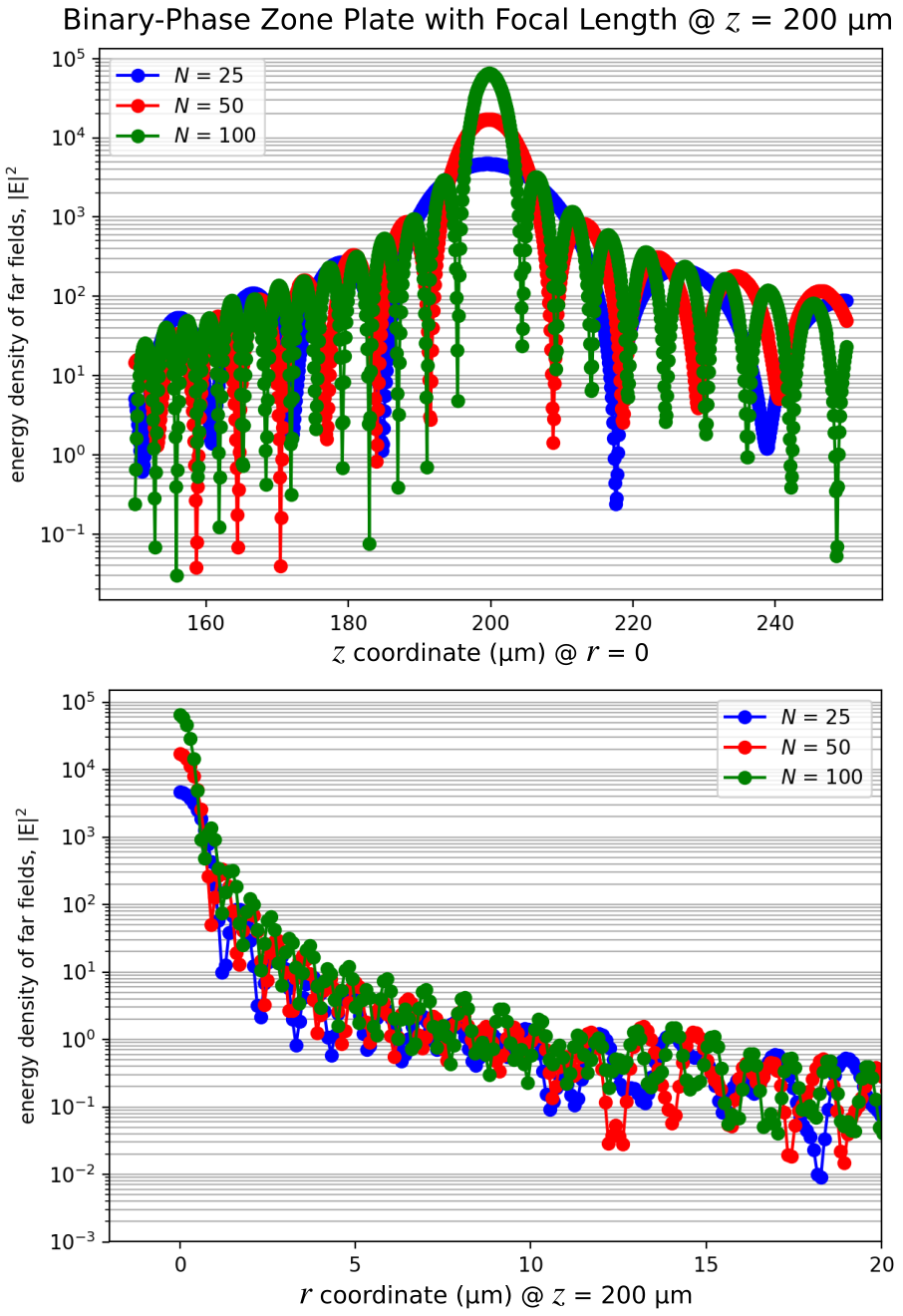
"Shown below is the far-field energy-density profile around the focal length for both the *r* and *z* coordinate directions for three lens designs with $N$ of 25, 50, and 100. The focus becomes sharper with increasing $N$ due to the enhanced constructive interference of the diffracted beam. As the number of zones $N$ increases, the size of the focal spot (full width at half maximum) at $z = 200$ μm decreases as $1/\\sqrt{N}$ (see eq. 17 of the [reference](http://zoneplate.lbl.gov/theory)). This means that doubling the resolution (halving the spot width) requires quadrupling the number of zones.\n",
"\n",
""
]
}
],
"metadata": {
"kernelspec": {
"display_name": "Python 3",
"language": "python",
"name": "python3"
},
"language_info": {
"codemirror_mode": {
"name": "ipython",
"version": 3
},
"file_extension": ".py",
"mimetype": "text/x-python",
"name": "python",
"nbconvert_exporter": "python",
"pygments_lexer": "ipython3",
"version": "3.6.7"
}
},
"nbformat": 4,
"nbformat_minor": 2
}