{
"cells": [
{
"cell_type": "markdown",
"id": "0",
"metadata": {},
"source": [
"# Datacubes\n",
"\n",
"\n",
"\n",
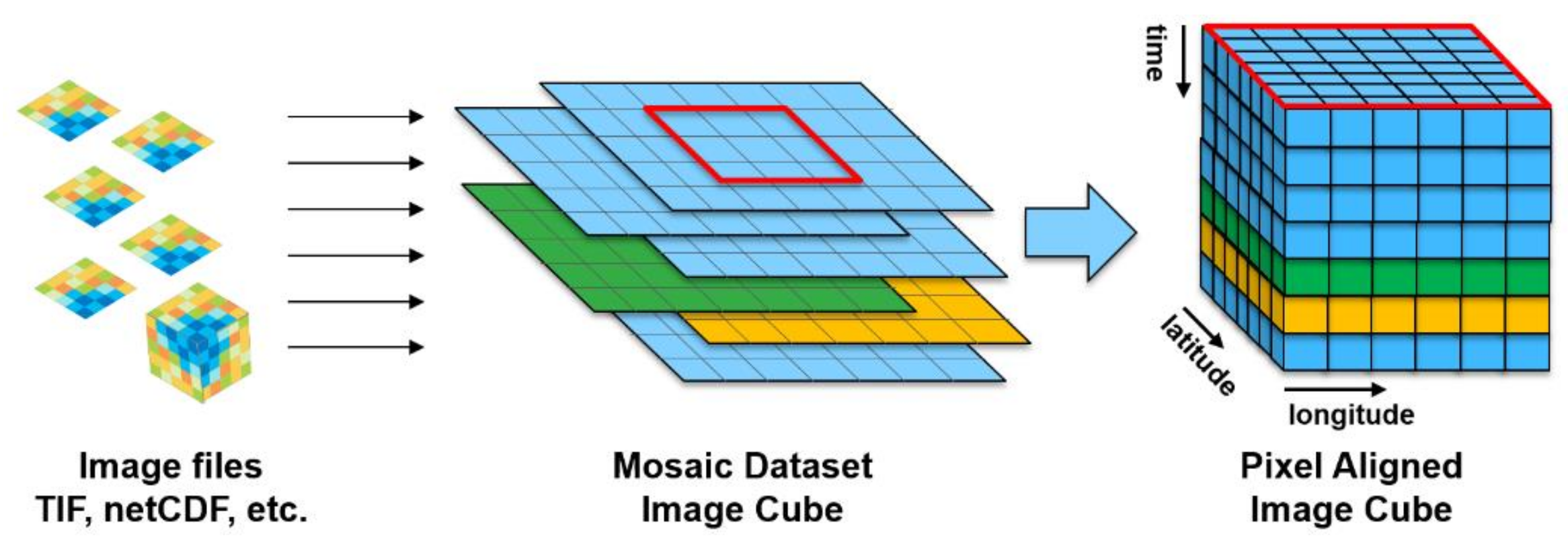
"In this notebook we discuss how we can easily compare images of two or more different time slices, satellites or other earth observation products. We limit our selves to products on a regular grid with an associated coordinate reference system (CRS), known as a raster. This means that each cell of the raster contains an attribute value and location coordinates. The process of combining such rasters to form datacubes is called raster stacking. We can have datacubes in many forms, such as the spatiotemporal datacube:\n",
"\n",
"$$Z = f(x,y,t) \\quad \\text{,}$$\n",
"\n",
"or when dealing with electromagnetic spectrum, the spectral wavelengths may form an additional dimension of a cube:\n",
"\n",
"$$Z = f(x,y,t, \\lambda ) \\quad \\text{.} $$\n",
"\n",
"We also have already encountered the case where $Z$ consists of multiple variables, such as seen in the `xarray` dataset.\n",
"\n",
"$${Z_1,Z_2,...,Z_3} = f(x,y,t) $$\n",
"\n",
"To perform raster stacking, we generally follow a certain routine (see also Figure 1).\n",
"\n",
"1. Collect data (GeoTIFF, NetCDF, Zarr)\n",
"2. Select an area of interest\n",
"3. Reproject all rasters to the same projection, resolution, and region\n",
"4. Stack the individual rasters\n",
"\n",
"To get the same projection, resolution, and region we have to resample one (or more) products. The desired projection, resolution, and region can be adopted from one of the original rasters or it can be a completely new projection of the data.\n",
"\n",
"\n",
"\n",
"*Figure 1: Stacking of arrays to form datacubes (source: https://eox.at)*.\n",
"\n",
"In this notebook we will study two different SAR products. SAR data from the Advanced Land Observing Satellite (Alos-2), which is a Japanese platform with an L-band sensor from the Japan Aerospace Exploration Agency (JAXA), and C-band data from the Copernicus Sentinel-1 mission. It is our goal to compare C- with L-band, so we need to somehow stack these arrays.\n",
"\n"
]
},
{
"cell_type": "code",
"execution_count": null,
"id": "1",
"metadata": {},
"outputs": [],
"source": [
"from functools import partial\n",
"from pathlib import Path\n",
"\n",
"import folium\n",
"import hvplot.xarray # noqa: F401\n",
"import numpy as np\n",
"import pandas as pd\n",
"import rioxarray # noqa: F401\n",
"import xarray as xr\n",
"from huggingface_hub import snapshot_download\n",
"from rasterio.enums import Resampling\n",
"from shapely import affinity\n",
"from shapely.geometry import box, mapping"
]
},
{
"cell_type": "markdown",
"id": "2",
"metadata": {},
"source": [
"## Download Data\n",
"\n",
"For this exercise we will download a set of GeoTIFF files for both Sentinel-1 and Alos-2, where each image has it's own timestamp for the acquisition.\n"
]
},
{
"cell_type": "code",
"execution_count": null,
"id": "3",
"metadata": {},
"outputs": [],
"source": [
"data_path = snapshot_download(\n",
" repo_id=\"martinschobben/microwave-remote-sensing\",\n",
" repo_type=\"dataset\",\n",
" allow_patterns=\"*.tif\",\n",
")\n",
"data_path = Path(data_path)"
]
},
{
"cell_type": "markdown",
"id": "4",
"metadata": {},
"source": [
"## Loading Data\n",
"\n",
"Before loading the data into memory we will first look at the area covered by the Sentinel-1 dataset on a map. This way we can select a region of interest for our hypothetical study. We will extract and transform the bounds of the data to longitude and latitude.\n"
]
},
{
"cell_type": "code",
"execution_count": null,
"id": "5",
"metadata": {},
"outputs": [],
"source": [
"bbox = xr.open_mfdataset(\n",
" (data_path / \"sentinel-1\").glob(\"**/*.tif\"),\n",
" engine=\"rasterio\",\n",
" combine=\"nested\",\n",
" concat_dim=\"band\",\n",
").rio.transform_bounds(\"EPSG:4326\")\n",
"\n",
"bbox = box(*bbox)\n",
"\n",
"map = folium.Map(\n",
" max_bounds=True,\n",
" location=[bbox.centroid.y, bbox.centroid.x],\n",
" scrollWheelZoom=False,\n",
")\n",
"\n",
"# bounds of image\n",
"folium.GeoJson(mapping(bbox), name=\"Area of Interest\", color=\"red\").add_to(map)\n",
"\n",
"# minimum longitude, minimum latitude, maximum longitude, maximum latitude\n",
"area_of_interest = box(10.3, 45.5, 10.6, 45.6)\n",
"\n",
"folium.GeoJson(mapping(area_of_interest), name=\"Area of Interest\").add_to(map)\n",
"\n",
"map"
]
},
{
"cell_type": "markdown",
"id": "6",
"metadata": {},
"source": [
"*Figure 2: Map of study area. Red rectangle is the area covered by the Sentinel-1 raster. Blue rectangle is the area of interest.*\n",
"\n",
"On the map we have drawn rectangles of the area covered by the images and of our selected study area. To prevent loading too much data we will now only load the data as defined by the blue rectangle on the `folium` map.\n",
"\n",
"The Sentinel-1 data is now stored on disk as separate two-dimensional GeoTIFF files with a certain timestamp. The following `s1_preprocess` function allows to load all files in one go as a spatiotemporal datacube. Basically, the preprocessing function helps reading the timestamp from the file and adds this as a new dimension to the array. The latter allows a concatenation procedure where all files are joined along the new time dimension. In addition by providing `area_of_interest.bounds` to the parameter `bbox` we will only load the data of the previously defined area of interest.\n"
]
},
{
"cell_type": "code",
"execution_count": null,
"id": "7",
"metadata": {},
"outputs": [],
"source": [
"def s1_preprocess(x, bbox, scale):\n",
" \"\"\"\n",
" Preprocess file.\n",
"\n",
" Parameters\n",
" ----------\n",
" x : xarray.Dataset\n",
" bbox: tuple\n",
" minimum longitude minimum latitude maximum longitude maximum latitude\n",
" scale: float\n",
" scaling factor\n",
" Returns\n",
" -------\n",
" xarray.Dataset\n",
" \"\"\"\n",
"\n",
" path = Path(x.encoding[\"source\"])\n",
" filename = path.name\n",
" x = x.rio.clip_box(*bbox, crs=\"EPSG:4326\")\n",
"\n",
" date_str = filename.split(\"_\")[0][1:]\n",
" time_str = filename.split(\"_\")[1][:6]\n",
" datetime_str = date_str + time_str\n",
" date = pd.to_datetime(datetime_str, format=\"%Y%m%d%H%M%S\")\n",
" x = x.expand_dims(dim={\"time\": [date]})\n",
"\n",
" x = (\n",
" x.rename({\"band_data\": \"s1_\" + path.parent.stem})\n",
" .squeeze(\"band\")\n",
" .drop_vars(\"band\")\n",
" )\n",
"\n",
" return x * scale"
]
},
{
"cell_type": "markdown",
"id": "8",
"metadata": {},
"source": [
"We load the data again with `open_mfdataset` and by providing the preprocess function, including the bounds of the area of interest and the scaling factor, as follows:\n"
]
},
{
"cell_type": "code",
"execution_count": null,
"id": "9",
"metadata": {},
"outputs": [],
"source": [
"partial_ = partial(s1_preprocess, bbox=area_of_interest.bounds, scale=0.01)\n",
"\n",
"s1_ds = xr.open_mfdataset(\n",
" (data_path / \"sentinel-1\").glob(\"**/*.tif\"),\n",
" engine=\"rasterio\",\n",
" combine=\"nested\",\n",
" chunks=-1,\n",
" preprocess=partial_,\n",
")"
]
},
{
"cell_type": "markdown",
"id": "10",
"metadata": {},
"source": [
"## Unlocking Geospatial Information\n",
"\n",
"To enable further stacking of ALOS-2 and Sentinel-1 data we need to know some more information about the raster. Hence we define the following function `print_raster` to get the projection (CRS), resolution, and region (bounds). The function leverages the functionality of `rioxarray`; a package for rasters.\n"
]
},
{
"cell_type": "code",
"execution_count": null,
"id": "11",
"metadata": {},
"outputs": [],
"source": [
"def print_raster(raster, name):\n",
" \"\"\"\n",
" Print Raster Metadata\n",
"\n",
" Parameters\n",
" ----------\n",
" raster: xarray.DataArray|xarray.DataSet\n",
" raster to process\n",
" y: string\n",
" name of product\n",
" \"\"\"\n",
"\n",
" print(\n",
" f\"{name} Raster: \\n----------------\\n\"\n",
" f\"resolution: {raster.rio.resolution()} {raster.rio.crs.units_factor}\\n\" # noqa\n",
" f\"bounds: {raster.rio.bounds()}\\n\"\n",
" f\"CRS: {raster.rio.crs}\\n\"\n",
" )\n",
"\n",
"\n",
"print_raster(s1_ds, \"Sentinel-1\")"
]
},
{
"cell_type": "markdown",
"id": "12",
"metadata": {},
"source": [
"The CRS \"EPSG 27704\" is part of the EQUI7Grid. This grid provides equal-area tiles, meaning each tile represents the same area, which helps reducing distorsions. This feature is important for remote sensing as it reduces the so-called oversampling due to geometric distortions when projecting on a sphere. This particular projection is developed by TUWien.\n",
"\n",
"Now we will proceed with loading the ALOS-2 L-band data in much the same fashion as for Sentinel-1. Again timeslices are stored separately as individual GeoTIFFS and they need to be concatenated along the time dimension. We use a slightly different preprocessing function `alos_preprocess` for this purpose. The most notable difference of this function is the inclusion of a scaling factor for the 16-bit digital numbers (DN):\n",
"\n",
"$$\\gamma^0_T = 10 * log_{10}(\\text{DN}^2) - 83.0 \\,dB$$\n",
"\n",
"to correctly convert the integers to $\\gamma^0_T$ in the dB range.\n"
]
},
{
"cell_type": "code",
"execution_count": null,
"id": "13",
"metadata": {},
"outputs": [],
"source": [
"def alos_preprocess(x, bbox):\n",
" \"\"\"\n",
" Preprocess file.\n",
"\n",
" Parameters\n",
" ----------\n",
" x : xarray.Dataset\n",
" bbox: tuple\n",
" minimum longitude minimum latitude maximum longitude maximum latitude\n",
" Returns\n",
" -------\n",
" xarray.Dataset\n",
" \"\"\"\n",
"\n",
" path = Path(x.encoding[\"source\"])\n",
" filename = path.name\n",
" x = x.rio.clip_box(*bbox, crs=\"EPSG:4326\")\n",
"\n",
" date_str = filename.split(\"_\")[0][15:22]\n",
" date = pd.to_datetime(date_str, format=\"%y%m%d\")\n",
" x = x.expand_dims(dim={\"time\": [date]})\n",
"\n",
" x = (\n",
" x.rename({\"band_data\": \"alos_\" + path.parent.stem})\n",
" .squeeze(\"band\")\n",
" .drop_vars(\"band\")\n",
" )\n",
"\n",
" # conversion to dB scale of alos\n",
" return 10 * np.log10(x**2) - 83.0"
]
},
{
"cell_type": "markdown",
"id": "14",
"metadata": {},
"source": [
"Now we load the data with the `open_mfdataset` function of `xarray` and we provide the preprocessing function (see above), which includes the selection of the bounds of an area of interest and the extraction of time stamps from the file name.\n"
]
},
{
"cell_type": "code",
"execution_count": null,
"id": "15",
"metadata": {},
"outputs": [],
"source": [
"area_of_interest = affinity.scale(area_of_interest, xfact=1.7, yfact=1.7)\n",
"partial_ = partial(alos_preprocess, bbox=area_of_interest.bounds)\n",
"\n",
"alos_ds = xr.open_mfdataset(\n",
" (data_path / \"alos-2\").glob(\"**/*.tif\"),\n",
" engine=\"rasterio\",\n",
" combine=\"nested\",\n",
" chunks=-1,\n",
" preprocess=partial_,\n",
")"
]
},
{
"cell_type": "markdown",
"id": "16",
"metadata": {},
"source": [
"Also, for this dataset we will look at the metadata in order to compare it with Sentinel-1.\n"
]
},
{
"cell_type": "code",
"execution_count": null,
"id": "17",
"metadata": {},
"outputs": [],
"source": [
"print_raster(alos_ds, \"ALOS-2\")"
]
},
{
"cell_type": "markdown",
"id": "18",
"metadata": {},
"source": [
"## Reprojecting\n",
"\n",
"The ALOS-2 is projected on an UTM grid. We would therefore like to reproject this data to match the projection of Sentinel-1. Furthermore, we will upsample the data to match the Sentinel-1 sampling. The `rioxarray` package has a very convenient method that can do this all in one go:`reproject_match`. For continuous data it is best to use a bilinear resampling strategy. As always you have to consider again that we deal with values in the dB range, so we need to convert to the linear scale before bilinear resampling.\n"
]
},
{
"cell_type": "code",
"execution_count": null,
"id": "19",
"metadata": {},
"outputs": [],
"source": [
"alos_ds_lin = 10 ** (alos_ds / 10)\n",
"alos_ds_lin = alos_ds_lin.rio.reproject_match(\n",
" s1_ds,\n",
" resampling=Resampling.bilinear,\n",
")\n",
"alos_ds = 10 * np.log10(alos_ds_lin)"
]
},
{
"cell_type": "markdown",
"id": "20",
"metadata": {},
"source": [
"We will overwrite the coordinate values of ALOS-2 with those of Sentinel-1. If we would not do this last step, small errors in how the numbers are stored would prevent stacking of the rasters.\n"
]
},
{
"cell_type": "code",
"execution_count": null,
"id": "21",
"metadata": {},
"outputs": [],
"source": [
"alos_ds = alos_ds.assign_coords(\n",
" {\n",
" \"x\": s1_ds.x.data,\n",
" \"y\": s1_ds.y.data,\n",
" }\n",
")"
]
},
{
"cell_type": "markdown",
"id": "22",
"metadata": {},
"source": [
"Lastly, we will turn the `xarray.DataSet` to an `xarray.DataArray` where a new dimension will constitute the sensor for measurement (satellite + polarization).\n"
]
},
{
"cell_type": "code",
"execution_count": null,
"id": "23",
"metadata": {},
"outputs": [],
"source": [
"s1_da = s1_ds.to_array(dim=\"sensor\")\n",
"alos_da = alos_ds.to_array(dim=\"sensor\")\n",
"s1_da"
]
},
{
"cell_type": "markdown",
"id": "24",
"metadata": {},
"source": [
"## Stacking of Multiple Arrays\n",
"\n",
"Now we are finally ready to stack Sentinel-1 C-band and ALOS-2 L-band arrays with the function `concat` of `xarray`. Now we can use the newly defined `\"sensor\"` dimension to concatenate the two arrays.\n"
]
},
{
"cell_type": "code",
"execution_count": null,
"id": "25",
"metadata": {},
"outputs": [],
"source": [
"fused_da = xr.concat([s1_da, alos_da], dim=\"sensor\").rename(\"gam0\")\n",
"fused_da"
]
},
{
"cell_type": "markdown",
"id": "26",
"metadata": {},
"source": [
"The measurements for both satellites don't occur at the same time. Hence the cube is now padded with 2-D arrays entirely filled with NaN (Not A Number) for some time slices. As we have learned in notebook 2 we can use the `resample` method to make temporally coherent timeslices for each month. To deal with the dB scale backscatter values as well as the low number of observations per month we use a median of the samples. As taking the median only sorts the samples according to the sample quantiles we do not have to convert the observations to the linear scale.\n"
]
},
{
"cell_type": "code",
"execution_count": null,
"id": "27",
"metadata": {},
"outputs": [],
"source": [
"fused_da = fused_da.resample(time=\"ME\", skipna=True).median().compute()"
]
},
{
"cell_type": "markdown",
"id": "28",
"metadata": {},
"source": [
"We can plot each of the variables: \"ALOS-2\" and \"Sentinel-1\" to check our results.\n"
]
},
{
"cell_type": "code",
"execution_count": null,
"id": "29",
"metadata": {},
"outputs": [],
"source": [
"fused_da.hvplot.image(robust=True, data_aspect=1, cmap=\"Greys_r\", rasterize=True).opts(\n",
" frame_height=600, aspect=\"equal\"\n",
")"
]
},
{
"cell_type": "markdown",
"id": "30",
"metadata": {},
"source": [
"*Figure 3: Stacked array with ALOS-2 L-band and Sentinel-1 C-band $\\gamma^0_T (dB)$.*"
]
}
],
"metadata": {
"kernelspec": {
"display_name": "Python 3 (ipykernel)",
"language": "python",
"name": "python3"
},
"language_info": {
"codemirror_mode": {
"name": "ipython",
"version": 3
},
"file_extension": ".py",
"mimetype": "text/x-python",
"name": "python",
"nbconvert_exporter": "python",
"pygments_lexer": "ipython3",
"version": "3.11.11"
}
},
"nbformat": 4,
"nbformat_minor": 5
}