{
"cells": [
{
"cell_type": "markdown",
"id": "350e9532",
"metadata": {},
"source": [
"$$\n",
"\\newcommand{\\argmax}{arg\\,max}\n",
"\\newcommand{\\argmin}{arg\\,min}\n",
"$$"
]
},
{
"cell_type": "markdown",
"id": "b9f3625e",
"metadata": {},
"source": [
"\n",
"\n",
""
]
},
{
"cell_type": "markdown",
"id": "06110f25",
"metadata": {},
"source": [
"# Pandas for Panel Data\n",
"\n",
"\n",
""
]
},
{
"cell_type": "markdown",
"id": "3def4a4f",
"metadata": {},
"source": [
"## Contents\n",
"\n",
"- [Pandas for Panel Data](#Pandas-for-Panel-Data) \n",
" - [Overview](#Overview) \n",
" - [Slicing and Reshaping Data](#Slicing-and-Reshaping-Data) \n",
" - [Merging Dataframes and Filling NaNs](#Merging-Dataframes-and-Filling-NaNs) \n",
" - [Grouping and Summarizing Data](#Grouping-and-Summarizing-Data) \n",
" - [Final Remarks](#Final-Remarks) \n",
" - [Exercises](#Exercises) "
]
},
{
"cell_type": "markdown",
"id": "f6241184",
"metadata": {},
"source": [
"## Overview\n",
"\n",
"In an [earlier lecture on pandas](https://python-programming.quantecon.org/pandas.html), we looked at working with simple data sets.\n",
"\n",
"Econometricians often need to work with more complex data sets, such as panels.\n",
"\n",
"Common tasks include\n",
"\n",
"- Importing data, cleaning it and reshaping it across several axes. \n",
"- Selecting a time series or cross-section from a panel. \n",
"- Grouping and summarizing data. \n",
"\n",
"\n",
"`pandas` (derived from ‘panel’ and ‘data’) contains powerful and\n",
"easy-to-use tools for solving exactly these kinds of problems.\n",
"\n",
"In what follows, we will use a panel data set of real minimum wages from the OECD to create:\n",
"\n",
"- summary statistics over multiple dimensions of our data \n",
"- a time series of the average minimum wage of countries in the dataset \n",
"- kernel density estimates of wages by continent \n",
"\n",
"\n",
"We will begin by reading in our long format panel data from a CSV file and\n",
"reshaping the resulting `DataFrame` with `pivot_table` to build a `MultiIndex`.\n",
"\n",
"Additional detail will be added to our `DataFrame` using pandas’\n",
"`merge` function, and data will be summarized with the `groupby`\n",
"function."
]
},
{
"cell_type": "markdown",
"id": "c3437fb0",
"metadata": {},
"source": [
"## Slicing and Reshaping Data\n",
"\n",
"We will read in a dataset from the OECD of real minimum wages in 32\n",
"countries and assign it to `realwage`.\n",
"\n",
"The dataset can be accessed with the following link:"
]
},
{
"cell_type": "code",
"execution_count": null,
"id": "b038cc75",
"metadata": {
"hide-output": false
},
"outputs": [],
"source": [
"url1 = 'https://raw.githubusercontent.com/QuantEcon/lecture-python/master/source/_static/lecture_specific/pandas_panel/realwage.csv'"
]
},
{
"cell_type": "code",
"execution_count": null,
"id": "c3db3fd8",
"metadata": {
"hide-output": false
},
"outputs": [],
"source": [
"import pandas as pd\n",
"\n",
"# Display 6 columns for viewing purposes\n",
"pd.set_option('display.max_columns', 6)\n",
"\n",
"# Reduce decimal points to 2\n",
"pd.options.display.float_format = '{:,.2f}'.format\n",
"\n",
"realwage = pd.read_csv(url1)"
]
},
{
"cell_type": "markdown",
"id": "c0de794a",
"metadata": {},
"source": [
"Let’s have a look at what we’ve got to work with"
]
},
{
"cell_type": "code",
"execution_count": null,
"id": "ce8fac8e",
"metadata": {
"hide-output": false
},
"outputs": [],
"source": [
"realwage.head() # Show first 5 rows"
]
},
{
"cell_type": "markdown",
"id": "3116c0d3",
"metadata": {},
"source": [
"The data is currently in long format, which is difficult to analyze when there are several dimensions to the data.\n",
"\n",
"We will use `pivot_table` to create a wide format panel, with a `MultiIndex` to handle higher dimensional data.\n",
"\n",
"`pivot_table` arguments should specify the data (values), the index, and the columns we want in our resulting dataframe.\n",
"\n",
"By passing a list in columns, we can create a `MultiIndex` in our column axis"
]
},
{
"cell_type": "code",
"execution_count": null,
"id": "f7840709",
"metadata": {
"hide-output": false
},
"outputs": [],
"source": [
"realwage = realwage.pivot_table(values='value',\n",
" index='Time',\n",
" columns=['Country', 'Series', 'Pay period'])\n",
"realwage.head()"
]
},
{
"cell_type": "markdown",
"id": "b679817d",
"metadata": {},
"source": [
"To more easily filter our time series data, later on, we will convert the index into a `DateTimeIndex`"
]
},
{
"cell_type": "code",
"execution_count": null,
"id": "c215ef3a",
"metadata": {
"hide-output": false
},
"outputs": [],
"source": [
"realwage.index = pd.to_datetime(realwage.index)\n",
"type(realwage.index)"
]
},
{
"cell_type": "markdown",
"id": "0b6bca29",
"metadata": {},
"source": [
"The columns contain multiple levels of indexing, known as a\n",
"`MultiIndex`, with levels being ordered hierarchically (Country >\n",
"Series > Pay period).\n",
"\n",
"A `MultiIndex` is the simplest and most flexible way to manage panel\n",
"data in pandas"
]
},
{
"cell_type": "code",
"execution_count": null,
"id": "abe85da9",
"metadata": {
"hide-output": false
},
"outputs": [],
"source": [
"type(realwage.columns)"
]
},
{
"cell_type": "code",
"execution_count": null,
"id": "4393226b",
"metadata": {
"hide-output": false
},
"outputs": [],
"source": [
"realwage.columns.names"
]
},
{
"cell_type": "markdown",
"id": "7b450e40",
"metadata": {},
"source": [
"Like before, we can select the country (the top level of our\n",
"`MultiIndex`)"
]
},
{
"cell_type": "code",
"execution_count": null,
"id": "f9285dff",
"metadata": {
"hide-output": false
},
"outputs": [],
"source": [
"realwage['United States'].head()"
]
},
{
"cell_type": "markdown",
"id": "20782333",
"metadata": {},
"source": [
"Stacking and unstacking levels of the `MultiIndex` will be used\n",
"throughout this lecture to reshape our dataframe into a format we need.\n",
"\n",
"`.stack()` rotates the lowest level of the column `MultiIndex` to\n",
"the row index (`.unstack()` works in the opposite direction - try it\n",
"out)"
]
},
{
"cell_type": "code",
"execution_count": null,
"id": "a3e748a0",
"metadata": {
"hide-output": false
},
"outputs": [],
"source": [
"realwage.stack(future_stack=True).head()"
]
},
{
"cell_type": "markdown",
"id": "9c479975",
"metadata": {},
"source": [
"We can also pass in an argument to select the level we would like to\n",
"stack"
]
},
{
"cell_type": "code",
"execution_count": null,
"id": "2205bdf9",
"metadata": {
"hide-output": false
},
"outputs": [],
"source": [
"realwage.stack(level='Country', future_stack=True).head()"
]
},
{
"cell_type": "markdown",
"id": "82259802",
"metadata": {},
"source": [
"Using a `DatetimeIndex` makes it easy to select a particular time\n",
"period.\n",
"\n",
"Selecting one year and stacking the two lower levels of the\n",
"`MultiIndex` creates a cross-section of our panel data"
]
},
{
"cell_type": "code",
"execution_count": null,
"id": "cc362c8b",
"metadata": {
"hide-output": false
},
"outputs": [],
"source": [
"realwage.loc['2015'].stack(level=(1, 2), future_stack=True).transpose().head()"
]
},
{
"cell_type": "markdown",
"id": "34d0378e",
"metadata": {},
"source": [
"For the rest of lecture, we will work with a dataframe of the hourly\n",
"real minimum wages across countries and time, measured in 2015 US\n",
"dollars.\n",
"\n",
"To create our filtered dataframe (`realwage_f`), we can use the `xs`\n",
"method to select values at lower levels in the multiindex, while keeping\n",
"the higher levels (countries in this case)"
]
},
{
"cell_type": "code",
"execution_count": null,
"id": "1d2598de",
"metadata": {
"hide-output": false
},
"outputs": [],
"source": [
"realwage_f = realwage.xs(('Hourly', 'In 2015 constant prices at 2015 USD exchange rates'),\n",
" level=('Pay period', 'Series'), axis=1)\n",
"realwage_f.head()"
]
},
{
"cell_type": "markdown",
"id": "48bcee87",
"metadata": {},
"source": [
"## Merging Dataframes and Filling NaNs\n",
"\n",
"Similar to relational databases like SQL, pandas has built in methods to\n",
"merge datasets together.\n",
"\n",
"Using country information from\n",
"[WorldData.info](https://www.worlddata.info/downloads/), we’ll add\n",
"the continent of each country to `realwage_f` with the `merge`\n",
"function.\n",
"\n",
"The dataset can be accessed with the following link:"
]
},
{
"cell_type": "code",
"execution_count": null,
"id": "074035b9",
"metadata": {
"hide-output": false
},
"outputs": [],
"source": [
"url2 = 'https://raw.githubusercontent.com/QuantEcon/lecture-python/master/source/_static/lecture_specific/pandas_panel/countries.csv'"
]
},
{
"cell_type": "code",
"execution_count": null,
"id": "17e3eca8",
"metadata": {
"hide-output": false
},
"outputs": [],
"source": [
"worlddata = pd.read_csv(url2, sep=';')\n",
"worlddata.head()"
]
},
{
"cell_type": "markdown",
"id": "c4a9413d",
"metadata": {},
"source": [
"First, we’ll select just the country and continent variables from\n",
"`worlddata` and rename the column to ‘Country’"
]
},
{
"cell_type": "code",
"execution_count": null,
"id": "dd3962d7",
"metadata": {
"hide-output": false
},
"outputs": [],
"source": [
"worlddata = worlddata[['Country (en)', 'Continent']]\n",
"worlddata = worlddata.rename(columns={'Country (en)': 'Country'})\n",
"worlddata.head()"
]
},
{
"cell_type": "markdown",
"id": "45d53d82",
"metadata": {},
"source": [
"We want to merge our new dataframe, `worlddata`, with `realwage_f`.\n",
"\n",
"The pandas `merge` function allows dataframes to be joined together by\n",
"rows.\n",
"\n",
"Our dataframes will be merged using country names, requiring us to use\n",
"the transpose of `realwage_f` so that rows correspond to country names\n",
"in both dataframes"
]
},
{
"cell_type": "code",
"execution_count": null,
"id": "84fda115",
"metadata": {
"hide-output": false
},
"outputs": [],
"source": [
"realwage_f.transpose().head()"
]
},
{
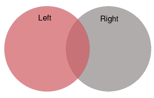
"cell_type": "markdown",
"id": "8b677dca",
"metadata": {},
"source": [
"We can use either left, right, inner, or outer join to merge our\n",
"datasets:\n",
"\n",
"- left join includes only countries from the left dataset \n",
"- right join includes only countries from the right dataset \n",
"- outer join includes countries that are in either the left and right datasets \n",
"- inner join includes only countries common to both the left and right datasets \n",
"\n",
"\n",
"By default, `merge` will use an inner join.\n",
"\n",
"Here we will pass `how='left'` to keep all countries in\n",
"`realwage_f`, but discard countries in `worlddata` that do not have\n",
"a corresponding data entry `realwage_f`.\n",
"\n",
"This is illustrated by the red shading in the following diagram\n",
"\n",
"\n",
"\n",
" \n",
"We will also need to specify where the country name is located in each\n",
"dataframe, which will be the `key` that is used to merge the\n",
"dataframes ‘on’.\n",
"\n",
"Our ‘left’ dataframe (`realwage_f.transpose()`) contains countries in\n",
"the index, so we set `left_index=True`.\n",
"\n",
"Our ‘right’ dataframe (`worlddata`) contains countries in the\n",
"‘Country’ column, so we set `right_on='Country'`"
]
},
{
"cell_type": "code",
"execution_count": null,
"id": "dd36c50b",
"metadata": {
"hide-output": false
},
"outputs": [],
"source": [
"merged = pd.merge(realwage_f.transpose(), worlddata,\n",
" how='left', left_index=True, right_on='Country')\n",
"merged.head()"
]
},
{
"cell_type": "markdown",
"id": "020f99f2",
"metadata": {},
"source": [
"Countries that appeared in `realwage_f` but not in `worlddata` will\n",
"have `NaN` in the Continent column.\n",
"\n",
"To check whether this has occurred, we can use `.isnull()` on the\n",
"continent column and filter the merged dataframe"
]
},
{
"cell_type": "code",
"execution_count": null,
"id": "e03c0043",
"metadata": {
"hide-output": false
},
"outputs": [],
"source": [
"merged[merged['Continent'].isnull()]"
]
},
{
"cell_type": "markdown",
"id": "db24d85c",
"metadata": {},
"source": [
"We have three missing values!\n",
"\n",
"One option to deal with NaN values is to create a dictionary containing\n",
"these countries and their respective continents.\n",
"\n",
"`.map()` will match countries in `merged['Country']` with their\n",
"continent from the dictionary.\n",
"\n",
"Notice how countries not in our dictionary are mapped with `NaN`"
]
},
{
"cell_type": "code",
"execution_count": null,
"id": "650292f3",
"metadata": {
"hide-output": false
},
"outputs": [],
"source": [
"missing_continents = {'Korea': 'Asia',\n",
" 'Russian Federation': 'Europe',\n",
" 'Slovak Republic': 'Europe'}\n",
"\n",
"merged['Country'].map(missing_continents)"
]
},
{
"cell_type": "markdown",
"id": "3b43865c",
"metadata": {},
"source": [
"We don’t want to overwrite the entire series with this mapping.\n",
"\n",
"`.fillna()` only fills in `NaN` values in `merged['Continent']`\n",
"with the mapping, while leaving other values in the column unchanged"
]
},
{
"cell_type": "code",
"execution_count": null,
"id": "38fe52a6",
"metadata": {
"hide-output": false
},
"outputs": [],
"source": [
"merged['Continent'] = merged['Continent'].fillna(merged['Country'].map(missing_continents))\n",
"\n",
"# Check for whether continents were correctly mapped\n",
"\n",
"merged[merged['Country'] == 'Korea']"
]
},
{
"cell_type": "markdown",
"id": "57b00180",
"metadata": {},
"source": [
"We will also combine the Americas into a single continent - this will make our visualization nicer later on.\n",
"\n",
"To do this, we will use `.replace()` and loop through a list of the continent values we want to replace"
]
},
{
"cell_type": "code",
"execution_count": null,
"id": "e67751b1",
"metadata": {
"hide-output": false
},
"outputs": [],
"source": [
"replace = ['Central America', 'North America', 'South America']\n",
"\n",
"for country in replace:\n",
" merged.Continent = merged.Continent.replace(to_replace=country,\n",
" value='America')"
]
},
{
"cell_type": "markdown",
"id": "98c7d2dc",
"metadata": {},
"source": [
"Now that we have all the data we want in a single `DataFrame`, we will\n",
"reshape it back into panel form with a `MultiIndex`.\n",
"\n",
"We should also ensure to sort the index using `.sort_index()` so that we\n",
"can efficiently filter our dataframe later on.\n",
"\n",
"By default, levels will be sorted top-down"
]
},
{
"cell_type": "code",
"execution_count": null,
"id": "9802d7b4",
"metadata": {
"hide-output": false
},
"outputs": [],
"source": [
"merged = merged.set_index(['Continent', 'Country']).sort_index()\n",
"merged.head()"
]
},
{
"cell_type": "markdown",
"id": "0cda397d",
"metadata": {},
"source": [
"While merging, we lost our `DatetimeIndex`, as we merged columns that\n",
"were not in datetime format"
]
},
{
"cell_type": "code",
"execution_count": null,
"id": "cff0b063",
"metadata": {
"hide-output": false
},
"outputs": [],
"source": [
"merged.columns"
]
},
{
"cell_type": "markdown",
"id": "106edc20",
"metadata": {},
"source": [
"Now that we have set the merged columns as the index, we can recreate a\n",
"`DatetimeIndex` using `.to_datetime()`"
]
},
{
"cell_type": "code",
"execution_count": null,
"id": "5e29e6a5",
"metadata": {
"hide-output": false
},
"outputs": [],
"source": [
"merged.columns = pd.to_datetime(merged.columns)\n",
"merged.columns = merged.columns.rename('Time')\n",
"merged.columns"
]
},
{
"cell_type": "markdown",
"id": "c94ee947",
"metadata": {},
"source": [
"The `DatetimeIndex` tends to work more smoothly in the row axis, so we\n",
"will go ahead and transpose `merged`"
]
},
{
"cell_type": "code",
"execution_count": null,
"id": "bda26c6f",
"metadata": {
"hide-output": false
},
"outputs": [],
"source": [
"merged = merged.transpose()\n",
"merged.head()"
]
},
{
"cell_type": "markdown",
"id": "5ac318b2",
"metadata": {},
"source": [
"## Grouping and Summarizing Data\n",
"\n",
"Grouping and summarizing data can be particularly useful for\n",
"understanding large panel datasets.\n",
"\n",
"A simple way to summarize data is to call an [aggregation\n",
"method](https://pandas.pydata.org/pandas-docs/stable/getting_started/intro_tutorials/06_calculate_statistics.html)\n",
"on the dataframe, such as `.mean()` or `.max()`.\n",
"\n",
"For example, we can calculate the average real minimum wage for each\n",
"country over the period 2006 to 2016 (the default is to aggregate over\n",
"rows)"
]
},
{
"cell_type": "code",
"execution_count": null,
"id": "6dd243cc",
"metadata": {
"hide-output": false
},
"outputs": [],
"source": [
"merged.mean().head(10)"
]
},
{
"cell_type": "markdown",
"id": "c3f111ae",
"metadata": {},
"source": [
"Using this series, we can plot the average real minimum wage over the\n",
"past decade for each country in our data set"
]
},
{
"cell_type": "code",
"execution_count": null,
"id": "6e540f7c",
"metadata": {
"hide-output": false
},
"outputs": [],
"source": [
"import matplotlib.pyplot as plt\n",
"import seaborn as sns\n",
"sns.set_theme()"
]
},
{
"cell_type": "code",
"execution_count": null,
"id": "f943465e",
"metadata": {
"hide-output": false
},
"outputs": [],
"source": [
"merged.mean().sort_values(ascending=False).plot(kind='bar',\n",
" title=\"Average real minimum wage 2006 - 2016\")\n",
"\n",
"# Set country labels\n",
"country_labels = merged.mean().sort_values(ascending=False).index.get_level_values('Country').tolist()\n",
"plt.xticks(range(0, len(country_labels)), country_labels)\n",
"plt.xlabel('Country')\n",
"\n",
"plt.show()"
]
},
{
"cell_type": "markdown",
"id": "725280fc",
"metadata": {},
"source": [
"Passing in `axis=1` to `.mean()` will aggregate over columns (giving\n",
"the average minimum wage for all countries over time)"
]
},
{
"cell_type": "code",
"execution_count": null,
"id": "2c471136",
"metadata": {
"hide-output": false
},
"outputs": [],
"source": [
"merged.mean(axis=1).head()"
]
},
{
"cell_type": "markdown",
"id": "8b792f7f",
"metadata": {},
"source": [
"We can plot this time series as a line graph"
]
},
{
"cell_type": "code",
"execution_count": null,
"id": "7ab6f47c",
"metadata": {
"hide-output": false
},
"outputs": [],
"source": [
"merged.mean(axis=1).plot()\n",
"plt.title('Average real minimum wage 2006 - 2016')\n",
"plt.ylabel('2015 USD')\n",
"plt.xlabel('Year')\n",
"plt.show()"
]
},
{
"cell_type": "markdown",
"id": "1dfe9f2c",
"metadata": {},
"source": [
"We can also specify a level of the `MultiIndex` (in the column axis)\n",
"to aggregate over"
]
},
{
"cell_type": "code",
"execution_count": null,
"id": "8e5cf319",
"metadata": {
"hide-output": false
},
"outputs": [],
"source": [
"merged.T.groupby(level='Continent').mean().T.head()"
]
},
{
"cell_type": "markdown",
"id": "7af4f7ba",
"metadata": {},
"source": [
"We can plot the average minimum wages in each continent as a time series"
]
},
{
"cell_type": "code",
"execution_count": null,
"id": "9ecb66be",
"metadata": {
"hide-output": false
},
"outputs": [],
"source": [
"merged.T.groupby(level='Continent').mean().T.plot()\n",
"plt.title('Average real minimum wage')\n",
"plt.ylabel('2015 USD')\n",
"plt.xlabel('Year')\n",
"plt.show()"
]
},
{
"cell_type": "markdown",
"id": "cef35611",
"metadata": {},
"source": [
"We will drop Australia as a continent for plotting purposes"
]
},
{
"cell_type": "code",
"execution_count": null,
"id": "5837490b",
"metadata": {
"hide-output": false
},
"outputs": [],
"source": [
"merged = merged.drop('Australia', level='Continent', axis=1)\n",
"merged.T.groupby(level='Continent').mean().T.plot()\n",
"plt.title('Average real minimum wage')\n",
"plt.ylabel('2015 USD')\n",
"plt.xlabel('Year')\n",
"plt.show()"
]
},
{
"cell_type": "markdown",
"id": "92df7c27",
"metadata": {},
"source": [
"`.describe()` is useful for quickly retrieving a number of common\n",
"summary statistics"
]
},
{
"cell_type": "code",
"execution_count": null,
"id": "a100f96a",
"metadata": {
"hide-output": false
},
"outputs": [],
"source": [
"merged.stack(future_stack=True).describe()"
]
},
{
"cell_type": "markdown",
"id": "7cd5404a",
"metadata": {},
"source": [
"This is a simplified way to use `groupby`.\n",
"\n",
"Using `groupby` generally follows a ‘split-apply-combine’ process:\n",
"\n",
"- split: data is grouped based on one or more keys \n",
"- apply: a function is called on each group independently \n",
"- combine: the results of the function calls are combined into a new data structure \n",
"\n",
"\n",
"The `groupby` method achieves the first step of this process, creating\n",
"a new `DataFrameGroupBy` object with data split into groups.\n",
"\n",
"Let’s split `merged` by continent again, this time using the\n",
"`groupby` function, and name the resulting object `grouped`"
]
},
{
"cell_type": "code",
"execution_count": null,
"id": "76c971b9",
"metadata": {
"hide-output": false
},
"outputs": [],
"source": [
"grouped = merged.T.groupby(level='Continent')\n",
"grouped"
]
},
{
"cell_type": "markdown",
"id": "46105b98",
"metadata": {},
"source": [
"Calling an aggregation method on the object applies the function to each\n",
"group, the results of which are combined in a new data structure.\n",
"\n",
"For example, we can return the number of countries in our dataset for\n",
"each continent using `.size()`.\n",
"\n",
"In this case, our new data structure is a `Series`"
]
},
{
"cell_type": "code",
"execution_count": null,
"id": "2669d8c4",
"metadata": {
"hide-output": false
},
"outputs": [],
"source": [
"grouped.size()"
]
},
{
"cell_type": "markdown",
"id": "df34fc80",
"metadata": {},
"source": [
"Calling `.get_group()` to return just the countries in a single group,\n",
"we can create a kernel density estimate of the distribution of real\n",
"minimum wages in 2016 for each continent.\n",
"\n",
"`grouped.groups.keys()` will return the keys from the `groupby`\n",
"object"
]
},
{
"cell_type": "code",
"execution_count": null,
"id": "6ffe0d5e",
"metadata": {
"hide-output": false
},
"outputs": [],
"source": [
"continents = grouped.groups.keys()\n",
"\n",
"for continent in continents:\n",
" sns.kdeplot(grouped.get_group(continent).T.loc['2015'].unstack(), label=continent, fill=True)\n",
"\n",
"plt.title('Real minimum wages in 2015')\n",
"plt.xlabel('US dollars')\n",
"plt.legend()\n",
"plt.show()"
]
},
{
"cell_type": "markdown",
"id": "9de4b42a",
"metadata": {},
"source": [
"## Final Remarks\n",
"\n",
"This lecture has provided an introduction to some of pandas’ more\n",
"advanced features, including multiindices, merging, grouping and\n",
"plotting.\n",
"\n",
"Other tools that may be useful in panel data analysis include [xarray](https://docs.xarray.dev/en/stable/), a python package that\n",
"extends pandas to N-dimensional data structures."
]
},
{
"cell_type": "markdown",
"id": "956ff5ad",
"metadata": {},
"source": [
"## Exercises"
]
},
{
"cell_type": "markdown",
"id": "3b567282",
"metadata": {},
"source": [
"## Exercise 85.1\n",
"\n",
"In these exercises, you’ll work with a dataset of employment rates\n",
"in Europe by age and sex from [Eurostat](https://ec.europa.eu/eurostat/data/database).\n",
"\n",
"The dataset can be accessed with the following link:"
]
},
{
"cell_type": "code",
"execution_count": null,
"id": "94332f7c",
"metadata": {
"hide-output": false
},
"outputs": [],
"source": [
"url3 = 'https://github.com/QuantEcon/lecture-python.myst/raw/refs/heads/main/lectures/_static/lecture_specific/pandas_panel/employ.csv'"
]
},
{
"cell_type": "markdown",
"id": "c70876b4",
"metadata": {},
"source": [
"Reading in the CSV file returns a panel dataset in long format. Use `.pivot_table()` to construct\n",
"a wide format dataframe with a `MultiIndex` in the columns.\n",
"\n",
"Start off by exploring the dataframe and the variables available in the\n",
"`MultiIndex` levels.\n",
"\n",
"Write a program that quickly returns all values in the `MultiIndex`."
]
},
{
"cell_type": "markdown",
"id": "8ee76ebf",
"metadata": {},
"source": [
"## Solution"
]
},
{
"cell_type": "code",
"execution_count": null,
"id": "f0aab7d0",
"metadata": {
"hide-output": false
},
"outputs": [],
"source": [
"employ = pd.read_csv(url3)\n",
"employ = employ.pivot_table(values='Value',\n",
" index=['DATE'],\n",
" columns=['UNIT','AGE', 'SEX', 'INDIC_EM', 'GEO'])\n",
"employ.index = pd.to_datetime(employ.index) # ensure that dates are datetime format\n",
"employ.head()"
]
},
{
"cell_type": "markdown",
"id": "d7c5c20b",
"metadata": {},
"source": [
"This is a large dataset so it is useful to explore the levels and\n",
"variables available"
]
},
{
"cell_type": "code",
"execution_count": null,
"id": "1b0326f7",
"metadata": {
"hide-output": false
},
"outputs": [],
"source": [
"employ.columns.names"
]
},
{
"cell_type": "markdown",
"id": "0bcb752d",
"metadata": {},
"source": [
"Variables within levels can be quickly retrieved with a loop"
]
},
{
"cell_type": "code",
"execution_count": null,
"id": "f936722f",
"metadata": {
"hide-output": false
},
"outputs": [],
"source": [
"for name in employ.columns.names:\n",
" print(name, employ.columns.get_level_values(name).unique())"
]
},
{
"cell_type": "markdown",
"id": "37284eea",
"metadata": {},
"source": [
"## Exercise 85.2\n",
"\n",
"Filter the above dataframe to only include employment as a percentage of\n",
"‘active population’.\n",
"\n",
"Create a grouped boxplot using `seaborn` of employment rates in 2015\n",
"by age group and sex.\n",
"\n",
"`GEO` includes both areas and countries."
]
},
{
"cell_type": "markdown",
"id": "d2d02920",
"metadata": {},
"source": [
"## Solution\n",
"\n",
"To easily filter by country, swap `GEO` to the top level and sort the\n",
"`MultiIndex`"
]
},
{
"cell_type": "code",
"execution_count": null,
"id": "4dde17e9",
"metadata": {
"hide-output": false
},
"outputs": [],
"source": [
"employ.columns = employ.columns.swaplevel(0,-1)\n",
"employ = employ.sort_index(axis=1)"
]
},
{
"cell_type": "markdown",
"id": "1b8efc96",
"metadata": {},
"source": [
"We need to get rid of a few items in `GEO` which are not countries.\n",
"\n",
"A fast way to get rid of the EU areas is to use a list comprehension to\n",
"find the level values in `GEO` that begin with ‘Euro’"
]
},
{
"cell_type": "code",
"execution_count": null,
"id": "4dc1ee4a",
"metadata": {
"hide-output": false
},
"outputs": [],
"source": [
"geo_list = employ.columns.get_level_values('GEO').unique().tolist()\n",
"countries = [x for x in geo_list if not x.startswith('Euro')]\n",
"employ = employ[countries]\n",
"employ.columns.get_level_values('GEO').unique()"
]
},
{
"cell_type": "markdown",
"id": "ebf54eee",
"metadata": {},
"source": [
"Select only percentage employed in the active population from the\n",
"dataframe"
]
},
{
"cell_type": "code",
"execution_count": null,
"id": "06bcafa7",
"metadata": {
"hide-output": false
},
"outputs": [],
"source": [
"employ_f = employ.xs(('Percentage of total population', 'Active population'),\n",
" level=('UNIT', 'INDIC_EM'),\n",
" axis=1)\n",
"employ_f.head()"
]
},
{
"cell_type": "markdown",
"id": "74089bff",
"metadata": {},
"source": [
"Drop the ‘Total’ value before creating the grouped boxplot"
]
},
{
"cell_type": "code",
"execution_count": null,
"id": "a4642628",
"metadata": {
"hide-output": false
},
"outputs": [],
"source": [
"employ_f = employ_f.drop('Total', level='SEX', axis=1)"
]
},
{
"cell_type": "code",
"execution_count": null,
"id": "c6075544",
"metadata": {
"hide-output": false
},
"outputs": [],
"source": [
"box = employ_f.loc['2015'].unstack().reset_index()\n",
"sns.boxplot(x=\"AGE\", y=0, hue=\"SEX\", data=box, palette=(\"husl\"), showfliers=False)\n",
"plt.xlabel('')\n",
"plt.xticks(rotation=35)\n",
"plt.ylabel('Percentage of population (%)')\n",
"plt.title('Employment in Europe (2015)')\n",
"plt.legend(bbox_to_anchor=(1,0.5))\n",
"plt.show()"
]
}
],
"metadata": {
"date": 1770028422.8261838,
"filename": "pandas_panel.md",
"kernelspec": {
"display_name": "Python",
"language": "python3",
"name": "python3"
},
"title": "Pandas for Panel Data"
},
"nbformat": 4,
"nbformat_minor": 5
}