# List of `RatInABox` plotting functions:
In this markdown we describe teh plotting functions available with `RatInABox`. The following definitions hold:
* `Env`: a 2D `Environment()` class with a wall and solid boundary conditions
* `Env1D`: a 1D `Environment()` class with periodic boundary conditions
# `Environment`
## `Environment.plot_environment()`
Displays the environment. Works for both 1 or 2D environments.
Examples:
* `Env.plot_environment()`
 # `Agent`
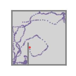
## `Agent.plot_trajectory()`
Plots the agent trajectory. Works for 1 or 2D.
* `Ag.plot_trajectory(t_end=120)`
# `Agent`
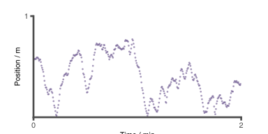
## `Agent.plot_trajectory()`
Plots the agent trajectory. Works for 1 or 2D.
* `Ag.plot_trajectory(t_end=120)`
 * `Ag1D.plot_trajectory(t_end=120)`
 ## `Agent.animate_trajectory()`
Makes an animation of the agents trajectory.
## `Agent.animate_trajectory()`
Makes an animation of the agents trajectory.
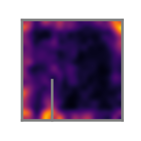
 ## `Agent.plot_position_heatmap()`
Plots a heatmap of the Agents past locations (2D and 1D example shown)
## `Agent.plot_position_heatmap()`
Plots a heatmap of the Agents past locations (2D and 1D example shown)
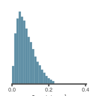
 ## `Agent.plot_histogram_of_speeds()`
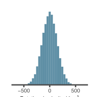
 ## `Agent.plot_histogram_of_rotational_velocities()`
 # `Neurons`
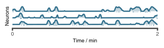
## `Neurons.plot_rate_timeseries()`
Plots a timeseries of the firing rates
# `Neurons`
## `Neurons.plot_rate_timeseries()`
Plots a timeseries of the firing rates
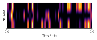
 ## `Neurons.plot_rate_timeseries(imshow=True)`
Plots a timeseries of the firing rates as an image
## `Neurons.plot_rate_timeseries(imshow=True)`
Plots a timeseries of the firing rates as an image
 Plots a timeseries of the firing rates
## `Neurons.animate_rate_timeseries()`
Makes an animation of the firing rates timeseries
Plots a timeseries of the firing rates
## `Neurons.animate_rate_timeseries()`
Makes an animation of the firing rates timeseries
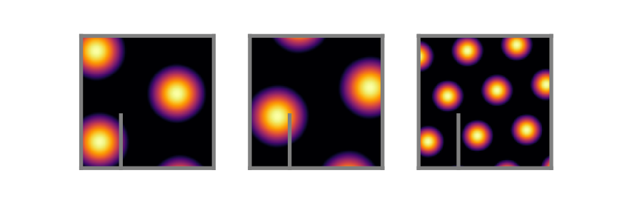
 ## `Neurons.plot_rate_map()`
Depending on the parameters passed this function will either
1. Analytically calculate the rate map (`method = 'analytic'`),
2. Infer the rate map from past activity (`method = 'history'`) or
3. Plot the observed spikes (`spikes=True`).
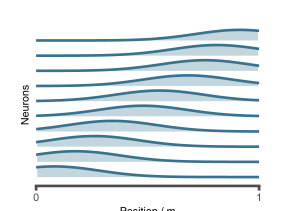
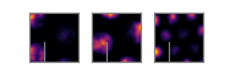
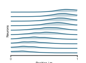
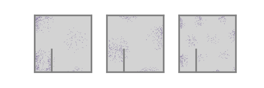
As an example here we show this function for a set of 3 (two dimensional) grid cells and 10 (one-dimensional) place cells.
* `Neurons.plot_rate_map(method=`analytic`)
## `Neurons.plot_rate_map()`
Depending on the parameters passed this function will either
1. Analytically calculate the rate map (`method = 'analytic'`),
2. Infer the rate map from past activity (`method = 'history'`) or
3. Plot the observed spikes (`spikes=True`).
As an example here we show this function for a set of 3 (two dimensional) grid cells and 10 (one-dimensional) place cells.
* `Neurons.plot_rate_map(method=`analytic`)
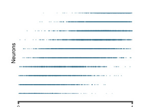
 * `Neurons.plot_rate_map(method=`history`)
 * `Neurons.plot_rate_map(method=`neither`, spikes=True)
 ## `PlaceCells.plot_place_cell_locations()`
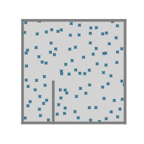
Scatters where the place cells are centres
## `PlaceCells.plot_place_cell_locations()`
Scatters where the place cells are centres
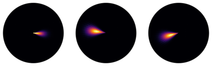
 ## `BoundaryVectorCells.plot_BVC_receptive_field()`
 # Other details:
* All plotting functions return a tuple (`fig`, `ax`) of `matplotlib` figure objects.
* Most plotting functions support being passed `fig` and `ax` and will plot whatever it is they plot ontop of that. This means we can make:
1. Layered figures (e.g. plot a trajectory on top of a rate map):
```python
fig, ax = Neurons.plot_rate_map(chosen_neuron="1")
fig, ax = Ag.plot_trajectory(fig=fig, ax=ax)
```
# Other details:
* All plotting functions return a tuple (`fig`, `ax`) of `matplotlib` figure objects.
* Most plotting functions support being passed `fig` and `ax` and will plot whatever it is they plot ontop of that. This means we can make:
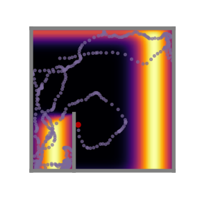
1. Layered figures (e.g. plot a trajectory on top of a rate map):
```python
fig, ax = Neurons.plot_rate_map(chosen_neuron="1")
fig, ax = Ag.plot_trajectory(fig=fig, ax=ax)
```
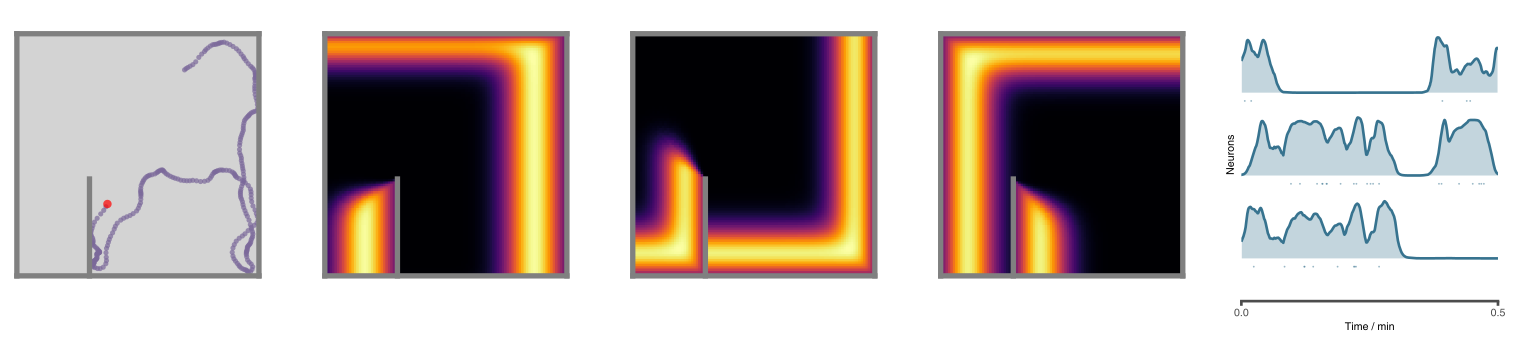
 2. Multipanel figures:
```python
fig, axes = plt.subplots(1,5,figsize=(20,4))
Ag.plot_trajectory(fig=fig,ax=axes[0])
Neurons.plot_rate_map(fig=fig,ax=[axes[1],axes[2],axes[3]],chosen_neurons='3') #<-- to plot more than 1 neuron pass an array of axes
Neurons.plot_rate_timeseries(fig=fig,ax=axes[4])
```
2. Multipanel figures:
```python
fig, axes = plt.subplots(1,5,figsize=(20,4))
Ag.plot_trajectory(fig=fig,ax=axes[0])
Neurons.plot_rate_map(fig=fig,ax=[axes[1],axes[2],axes[3]],chosen_neurons='3') #<-- to plot more than 1 neuron pass an array of axes
Neurons.plot_rate_timeseries(fig=fig,ax=axes[4])
```
 * For rate maps and timeseries' by default **all** the cells will be plotted. This may take a long time if the number of cells is large. Control this with the `chosen_neurons` argument
* We use the `matplotlib` wrapper [`tomplotlib`](https://github.com/RatInABox-Lab/tomplotlib) to format and save figures. This is not necesary for the workings of `ratinabox` but note your figures might look slightly different without it.
* For rate maps and timeseries' by default **all** the cells will be plotted. This may take a long time if the number of cells is large. Control this with the `chosen_neurons` argument
* We use the `matplotlib` wrapper [`tomplotlib`](https://github.com/RatInABox-Lab/tomplotlib) to format and save figures. This is not necesary for the workings of `ratinabox` but note your figures might look slightly different without it.