{
"cells": [
{
"cell_type": "markdown",
"metadata": {
"slideshow": {
"slide_type": "slide"
}
},
"source": [
"***\n",
"***\n",
"\n",
"\n",
"# Introduction to Gradient Descent\n",
"\n",
"The Idea Behind Gradient Descent 梯度下降\n",
"\n",
"***\n",
"***\n",
"\n"
]
},
{
"cell_type": "markdown",
"metadata": {
"slideshow": {
"slide_type": "subslide"
}
},
"source": [
" "
]
},
{
"cell_type": "markdown",
"metadata": {
"slideshow": {
"slide_type": "subslide"
}
},
"source": [
"
"
]
},
{
"cell_type": "markdown",
"metadata": {
"slideshow": {
"slide_type": "subslide"
}
},
"source": [
" \n",
"\n",
"\n",
"**如何找到最快下山的路?**\n",
"- 假设此时山上的浓雾很大,下山的路无法确定;\n",
"- 假设你摔不死!\n",
"\n",
" - 你只能利用自己周围的信息去找到下山的路径。\n",
" - 以你当前的位置为基准,寻找这个位置最陡峭的方向,从这个方向向下走。\n"
]
},
{
"cell_type": "markdown",
"metadata": {
"slideshow": {
"slide_type": "subslide"
}
},
"source": [
"
\n",
"\n",
"\n",
"**如何找到最快下山的路?**\n",
"- 假设此时山上的浓雾很大,下山的路无法确定;\n",
"- 假设你摔不死!\n",
"\n",
" - 你只能利用自己周围的信息去找到下山的路径。\n",
" - 以你当前的位置为基准,寻找这个位置最陡峭的方向,从这个方向向下走。\n"
]
},
{
"cell_type": "markdown",
"metadata": {
"slideshow": {
"slide_type": "subslide"
}
},
"source": [
" \n",
"**Gradient is the vector of partial derivatives**\n",
"\n",
"One approach to maximizing a function is to\n",
"- pick a random starting point, \n",
"- compute the gradient, \n",
"- take a small step in the direction of the gradient, and \n",
"- repeat with a new staring point.\n",
"\n"
]
},
{
"cell_type": "markdown",
"metadata": {
"slideshow": {
"slide_type": "subslide"
}
},
"source": [
"\n",
"\n",
"
\n",
"**Gradient is the vector of partial derivatives**\n",
"\n",
"One approach to maximizing a function is to\n",
"- pick a random starting point, \n",
"- compute the gradient, \n",
"- take a small step in the direction of the gradient, and \n",
"- repeat with a new staring point.\n",
"\n"
]
},
{
"cell_type": "markdown",
"metadata": {
"slideshow": {
"slide_type": "subslide"
}
},
"source": [
"\n",
"\n",
" \n",
"Let's represent parameters as $\\Theta$, learning rate as $\\alpha$, and gradient as $\\bigtriangledown J(\\Theta)$, "
]
},
{
"cell_type": "markdown",
"metadata": {
"slideshow": {
"slide_type": "subslide"
}
},
"source": [
"To the find the best model is an optimization problem\n",
"- “minimizes the error of the model” \n",
"- “maximizes the likelihood of the data.” "
]
},
{
"cell_type": "markdown",
"metadata": {
"slideshow": {
"slide_type": "subslide"
}
},
"source": [
"We’ll frequently need to maximize (or minimize) functions. \n",
"- to find the input vector v that produces the largest (or smallest) possible value.\n"
]
},
{
"cell_type": "markdown",
"metadata": {
"slideshow": {
"slide_type": "slide"
}
},
"source": [
"# Mathematics behind Gradient Descent\n",
"\n",
"A simple mathematical intuition behind one of the commonly used optimisation algorithms in Machine Learning.\n",
"\n",
"https://www.douban.com/note/713353797/"
]
},
{
"cell_type": "markdown",
"metadata": {
"slideshow": {
"slide_type": "subslide"
}
},
"source": [
"The cost or loss function:\n",
"\n",
"$$Cost = \\frac{1}{N} \\sum_{i = 1}^N (Y' -Y)^2$$"
]
},
{
"cell_type": "markdown",
"metadata": {
"slideshow": {
"slide_type": "subslide"
}
},
"source": [
"\n",
"\n",
"
\n",
"Let's represent parameters as $\\Theta$, learning rate as $\\alpha$, and gradient as $\\bigtriangledown J(\\Theta)$, "
]
},
{
"cell_type": "markdown",
"metadata": {
"slideshow": {
"slide_type": "subslide"
}
},
"source": [
"To the find the best model is an optimization problem\n",
"- “minimizes the error of the model” \n",
"- “maximizes the likelihood of the data.” "
]
},
{
"cell_type": "markdown",
"metadata": {
"slideshow": {
"slide_type": "subslide"
}
},
"source": [
"We’ll frequently need to maximize (or minimize) functions. \n",
"- to find the input vector v that produces the largest (or smallest) possible value.\n"
]
},
{
"cell_type": "markdown",
"metadata": {
"slideshow": {
"slide_type": "slide"
}
},
"source": [
"# Mathematics behind Gradient Descent\n",
"\n",
"A simple mathematical intuition behind one of the commonly used optimisation algorithms in Machine Learning.\n",
"\n",
"https://www.douban.com/note/713353797/"
]
},
{
"cell_type": "markdown",
"metadata": {
"slideshow": {
"slide_type": "subslide"
}
},
"source": [
"The cost or loss function:\n",
"\n",
"$$Cost = \\frac{1}{N} \\sum_{i = 1}^N (Y' -Y)^2$$"
]
},
{
"cell_type": "markdown",
"metadata": {
"slideshow": {
"slide_type": "subslide"
}
},
"source": [
"\n",
"\n",
" "
]
},
{
"cell_type": "markdown",
"metadata": {
"slideshow": {
"slide_type": "subslide"
}
},
"source": [
"Parameters with small changes:\n",
"$$ m_1 = m_0 - \\delta m, b_1 = b_0 - \\delta b$$\n",
"\n",
"The cost function J is a function of m and b:\n",
"\n",
"$$J_{m, b} = \\frac{1}{N} \\sum_{i = 1}^N (Y' -Y)^2 = \\frac{1}{N} \\sum_{i = 1}^N Error_i^2$$"
]
},
{
"cell_type": "markdown",
"metadata": {
"slideshow": {
"slide_type": "subslide"
}
},
"source": [
"$$\\frac{\\partial J}{\\partial m} = 2 Error \\frac{\\partial}{\\partial m}Error$$\n",
"\n",
"$$\\frac{\\partial J}{\\partial b} = 2 Error \\frac{\\partial}{\\partial b}Error$$"
]
},
{
"cell_type": "markdown",
"metadata": {
"slideshow": {
"slide_type": "subslide"
}
},
"source": [
"Let's fit the data with linear regression:\n",
"\n",
"$$\\frac{\\partial}{\\partial m}Error = \\frac{\\partial}{\\partial m}(Y' - Y) = \\frac{\\partial}{\\partial m}(mX + b - Y)$$\n",
"\n",
"Since $X, b, Y$ are constant:\n",
"\n",
"$$\\frac{\\partial}{\\partial m}Error = X$$"
]
},
{
"cell_type": "markdown",
"metadata": {
"slideshow": {
"slide_type": "subslide"
}
},
"source": [
"$$\\frac{\\partial}{\\partial b}Error = \\frac{\\partial}{\\partial b}(Y' - Y) = \\frac{\\partial}{\\partial b}(mX + b - Y)$$\n",
"\n",
"Since $X, m, Y$ are constant:\n",
"\n",
"$$\\frac{\\partial}{\\partial m}Error = 1$$"
]
},
{
"cell_type": "markdown",
"metadata": {
"slideshow": {
"slide_type": "subslide"
}
},
"source": [
"Thus:\n",
" \n",
"$$\\frac{\\partial J}{\\partial m} = 2 * Error * X$$\n",
"$$\\frac{\\partial J}{\\partial b} = 2 * Error$$"
]
},
{
"cell_type": "markdown",
"metadata": {
"slideshow": {
"slide_type": "subslide"
}
},
"source": [
"Let's get rid of the constant 2 and multiplying the learning rate $\\alpha$, who determines how large a step to take:\n",
"\n",
"$$\\frac{\\partial J}{\\partial m} = Error * X * \\alpha$$\n",
"$$\\frac{\\partial J}{\\partial b} = Error * \\alpha$$\n"
]
},
{
"cell_type": "markdown",
"metadata": {
"slideshow": {
"slide_type": "subslide"
}
},
"source": [
"Since $ m_1 = m_0 - \\delta m, b_1 = b_0 - \\delta b$:\n",
"\n",
"$$ m_1 = m_0 - Error * X * \\alpha$$\n",
"\n",
"$$b_1 = b_0 - Error * \\alpha$$\n",
"\n",
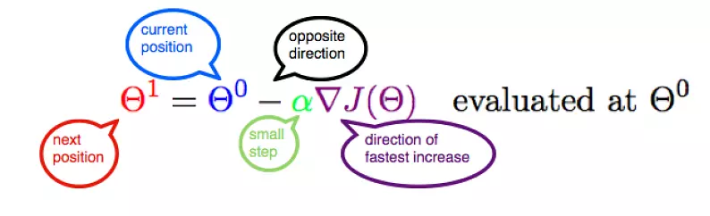
"**Notice** that the slope b can be viewed as the beta value for X = 1. Thus, the above two equations are in essence the same.\n",
"\n",
"Let's represent parameters as $\\Theta$, learning rate as $\\alpha$, and gradient as $\\bigtriangledown J(\\Theta)$, we have:\n",
"\n",
"\n",
"$$\\Theta_1 = \\Theta_0 - \\alpha \\bigtriangledown J(\\Theta)$$\n"
]
},
{
"cell_type": "markdown",
"metadata": {
"slideshow": {
"slide_type": "subslide"
}
},
"source": [
"\n",
"\n",
""
]
},
{
"cell_type": "markdown",
"metadata": {
"slideshow": {
"slide_type": "subslide"
}
},
"source": [
"Hence,to solve for the gradient, we iterate through our data points using our new $m$ and $b$ values and compute the partial derivatives. \n",
"\n",
"This new gradient tells us \n",
"- the slope of our cost function at our current position \n",
"- the direction we should move to update our parameters. \n",
"\n",
"- The size of our update is controlled by the learning rate."
]
},
{
"cell_type": "code",
"execution_count": 17,
"metadata": {
"ExecuteTime": {
"end_time": "2019-04-07T16:16:42.584919Z",
"start_time": "2019-04-07T16:16:42.573596Z"
},
"slideshow": {
"slide_type": "slide"
}
},
"outputs": [],
"source": [
"import numpy as np\n",
"\n",
"# Size of the points dataset.\n",
"m = 20\n",
"# Points x-coordinate and dummy value (x0, x1).\n",
"X0 = np.ones((m, 1))\n",
"X1 = np.arange(1, m+1).reshape(m, 1)\n",
"X = np.hstack((X0, X1))\n",
"# Points y-coordinate\n",
"y = np.array([3, 4, 5, 5, 2, 4, 7, 8, 11, 8, 12,\n",
" 11, 13, 13, 16, 17, 18, 17, 19, 21]).reshape(m, 1)\n",
"\n",
"# The Learning Rate alpha.\n",
"alpha = 0.01"
]
},
{
"cell_type": "code",
"execution_count": 18,
"metadata": {
"ExecuteTime": {
"end_time": "2019-04-07T16:17:04.134904Z",
"start_time": "2019-04-07T16:17:04.108505Z"
},
"slideshow": {
"slide_type": "subslide"
}
},
"outputs": [],
"source": [
"def error_function(theta, X, y):\n",
" '''Error function J definition.'''\n",
" diff = np.dot(X, theta) - y\n",
" return (1./2*m) * np.dot(np.transpose(diff), diff)\n",
"\n",
"def gradient_function(theta, X, y):\n",
" '''Gradient of the function J definition.'''\n",
" diff = np.dot(X, theta) - y\n",
" return (1./m) * np.dot(np.transpose(X), diff)\n",
"\n",
"def gradient_descent(X, y, alpha):\n",
" '''Perform gradient descent.'''\n",
" theta = np.array([1, 1]).reshape(2, 1)\n",
" gradient = gradient_function(theta, X, y)\n",
" while not np.all(np.absolute(gradient) <= 1e-5):\n",
" theta = theta - alpha * gradient\n",
" gradient = gradient_function(theta, X, y)\n",
" return theta\n",
"\n",
"# source:https://www.jianshu.com/p/c7e642877b0e"
]
},
{
"cell_type": "code",
"execution_count": 23,
"metadata": {
"ExecuteTime": {
"end_time": "2019-04-07T16:19:07.236028Z",
"start_time": "2019-04-07T16:19:07.171443Z"
},
"slideshow": {
"slide_type": "subslide"
}
},
"outputs": [
{
"name": "stdout",
"output_type": "stream",
"text": [
"Optimal parameters Theta: 0.5158328581734093 0.9699216324486175\n",
"Error function: 405.98496249324046\n"
]
}
],
"source": [
"optimal = gradient_descent(X, y, alpha)\n",
"print('Optimal parameters Theta:', optimal[0][0], optimal[1][0])\n",
"print('Error function:', error_function(optimal, X, y)[0,0])\n"
]
},
{
"cell_type": "markdown",
"metadata": {
"slideshow": {
"slide_type": "slide"
}
},
"source": [
"# This is the End!"
]
},
{
"cell_type": "markdown",
"metadata": {
"slideshow": {
"slide_type": "skip"
}
},
"source": [
"# Estimating the Gradient"
]
},
{
"cell_type": "markdown",
"metadata": {
"slideshow": {
"slide_type": "subslide"
}
},
"source": [
"If f is a function of one variable, its derivative at a point x measures how f(x) changes when we make a very small change to x. \n",
"\n",
"> It is defined as the limit of the difference quotients:\n",
"\n",
"\n",
"差商(difference quotient)就是因变量的改变量与自变量的改变量两者相除的商。"
]
},
{
"cell_type": "code",
"execution_count": 2,
"metadata": {
"ExecuteTime": {
"end_time": "2019-04-07T16:08:29.774271Z",
"start_time": "2019-04-07T16:08:29.771043Z"
},
"slideshow": {
"slide_type": "fragment"
}
},
"outputs": [],
"source": [
"def difference_quotient(f, x, h):\n",
" return (f(x + h) - f(x)) / h"
]
},
{
"cell_type": "markdown",
"metadata": {
"slideshow": {
"slide_type": "subslide"
}
},
"source": [
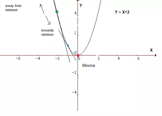
"For many functions it’s easy to exactly calculate derivatives. \n",
"\n",
"For example, the square function:\n",
"\n",
" def square(x): \n",
" return x * x\n",
"\n",
"has the derivative:\n",
" \n",
" def derivative(x): \n",
" return 2 * x"
]
},
{
"cell_type": "code",
"execution_count": 3,
"metadata": {
"ExecuteTime": {
"end_time": "2019-04-07T16:08:30.714322Z",
"start_time": "2019-04-07T16:08:30.709209Z"
},
"slideshow": {
"slide_type": "subslide"
}
},
"outputs": [],
"source": [
"def square(x):\n",
" return x * x\n",
"\n",
"def derivative(x):\n",
" return 2 * x\n",
"\n",
"derivative_estimate = lambda x: difference_quotient(square, x, h=0.00001)"
]
},
{
"cell_type": "code",
"execution_count": 9,
"metadata": {
"ExecuteTime": {
"end_time": "2019-04-07T16:09:28.375610Z",
"start_time": "2019-04-07T16:09:28.372132Z"
},
"slideshow": {
"slide_type": "fragment"
}
},
"outputs": [],
"source": [
"def sum_of_squares(v):\n",
" \"\"\"computes the sum of squared elements in v\"\"\"\n",
" return sum(v_i ** 2 for v_i in v)"
]
},
{
"cell_type": "code",
"execution_count": 12,
"metadata": {
"ExecuteTime": {
"end_time": "2019-04-07T16:11:00.628162Z",
"start_time": "2019-04-07T16:11:00.425853Z"
},
"slideshow": {
"slide_type": "subslide"
}
},
"outputs": [
{
"data": {
"image/png": "iVBORw0KGgoAAAANSUhEUgAAAXwAAAD8CAYAAAB0IB+mAAAABHNCSVQICAgIfAhkiAAAAAlwSFlzAAALEgAACxIB0t1+/AAAADl0RVh0U29mdHdhcmUAbWF0cGxvdGxpYiB2ZXJzaW9uIDMuMC4xLCBodHRwOi8vbWF0cGxvdGxpYi5vcmcvDW2N/gAAEdhJREFUeJzt3X+MHPV9xvHnqV2oRFFI6ws4gHsQuagGtW5ysUJFmxhoYqwIB1Qs548WRCSLNkhNlCgCUSWX5p+GiEaqGqAXFUErBLhpCRYQfgVHbqUAPiPjHxiD+RFhy4F1oLhVKiLg0z9mDHvHrnfuZmdm577vl7S63ZnxzFez6+fmZufzGUeEAAAL3681PQAAQD0IfABIBIEPAIkg8AEgEQQ+ACSCwAeARBD4AJAIAh8AEkHgA0AiFjc9gG5LliyJ8fHxpocBAK2yffv2wxExNmi5kQr88fFxTU9PNz0MAGgV2z8rshyndAAgEQQ+ACSCwAeARBD4AJAIAh8AEkHgA0BTrr9e2rJFkjQ5mU/bsiWbXgECHwCa8vGPS+vXS1u26JvfVBb269dn0ytA4ANAU1avljZtykJeyn5u2pRNrwCBDwANmZyUfP5q+XBHkuTDHfn81e+d3hkyAh8AGjI5KcWjWxRLsq4IsWRM8egWAh8AFpyj5+w3bcpeHz29k3+RO2wEPgA0Zdu2d8/Zf+Mbeu+c/rZtlWzOEVHJiudjYmIiaJ4GAHNje3tETAxajiN8AEgEgQ8AiSDwASARBD4AzFfNrRHKIvABYL5qbo1QFoEPAPNVc2uEsgh8AJinulsjlDWUwLd9i+1Xbe/umjZp+6DtHflj7TC2BQCjou7WCGUN6wj/Vklrekz/bkSszB/3D2lbADAaam6NUNZQAj8itkp6bRjrAoDWqLk1QllDa61ge1zSvRFxTv56UtIVko5Impb0lYh4/VjroLUCAMzdKLRWuEnSRyStlHRI0g29FrK90fa07elOp1PhcAAgbZUFfkS8EhFvR8Q7kr4vaVWf5aYiYiIiJsbGxqoaDgAkr7LAt7206+Ulknb3WxYAGtGyStmyhnVZ5h2SfirpLNsHbH9B0vW2d9neKWm1pC8PY1sAMDQtq5Qti374ANKWh7wPd7Lr6Ue4UrafUfjSFgBGWtsqZcsi8AEkq22VsmUR+ADS1bJK2bIIfADpalmlbFl8aQsALceXtgCAGQh8AEgEgQ+gvRKrlC2LwAfQXolVypZF4ANor5bdU7ZpBD6A1kqtUrYsAh9Aa6VWKVsWgQ+gvRKrlC2LwAfQXolVypZFpS0AtByVtgCAGQh8AEjEsG5xeIvtV23v7pr2W7Yftv1c/vODw9gWAGB+hnWEf6ukNbOmXSPpxxGxXNKP89cA8B5aI9RqKIEfEVslvTZr8jpJt+XPb5P0uWFsC8ACQmuEWlV5Dv/kiDiUP/+5pJMr3BaANqI1Qq1q+dI2sms/e17/aXuj7Wnb051Op47hABgRtEaoV5WB/4rtpZKU/3y110IRMRURExExMTY2VuFwAIwaWiPUq8rA3yzp8vz55ZLuqXBbANqI1gi1GtZlmXdI+qmks2wfsP0FSX8n6U9tPyfpwvw1ALyH1gi1orUCALQcrRUAADMQ+ACQCAIfwPxRKdsqBD6A+aNStlUIfADzR6VsqxD4AOaNStl2IfABzBuVsu1C4AOYPyplW4XABzB/VMq2CpW2ANByVNoCAGYg8AEgEQQ+ACSCwAdSRmuEpBD4QMpojZAUAh9IGa0RkkLgAwmjNUJaKg982y/Z3mV7h20usgdGCK0R0lLXEf7qiFhZpDAAQI1ojZAUTukAKaM1QlIqb61g+0VJr0sKSf8UEVP9lqW1AgDMXdHWCotrGMt5EXHQ9ockPWz7mYjYenSm7Y2SNkrSsmXLahgOAKSp8lM6EXEw//mqpLslrZo1fyoiJiJiYmxsrOrhAECyKg182yfYPvHoc0mflrS7ym0CSaFSFnNQ9RH+yZL+y/ZTkp6QdF9EPFDxNoF0UCmLOaj0HH5EvCDpD6rcBpC0GZWyHSplcUxclgm0GJWymAsCH2gxKmUxFwQ+0GZUymIOCHygzaiUxRxwE3MAaDluYg4AmIHAB4BEEPhAk6iURY0IfKBJVMqiRgQ+0CTuKYsaEfhAg6iURZ0IfKBBVMqiTgQ+0CQqZVEjAh9oEpWyqBGVtgDQclTaAgBmIPABIBGVB77tNbb32d5v+5qqtwcA6K3qm5gvkvQ9SRdJWiHp87ZXVLlNoFa0RkCLVH2Ev0rS/oh4ISJ+JelOSesq3iZQH1ojoEWqDvxTJb3c9fpAPg1YGGiNgBZp/Etb2xttT9ue7nQ6TQ8HmBNaI6BNqg78g5JO73p9Wj7tXRExFRETETExNjZW8XCA4aI1Atqk6sDfJmm57TNsHydpg6TNFW8TqA+tEdAilQZ+RLwl6WpJD0raK2lTROypcptArWiNgBahtQIAtBytFQAAMxD4AJAIAh9po1IWCSHwkTYqZZEQAh9po1IWCSHwkTQqZZESAh9Jo1IWKSHwkTYqZZEQAh9po1IWCaHSFgBajkpbAMAMBD4AJILAB4BEEPhoN1ojAIUR+Gg3WiMAhRH4aDdaIwCFEfhoNVojAMVVFvi2J20ftL0jf6ytaltIF60RgOKqPsL/bkSszB/3V7wtpIjWCEBhnNJBu9EaASisstYKticlXSHpiKRpSV+JiNeP9W9orQAAc1dLawXbj9je3eOxTtJNkj4iaaWkQ5Ju6LOOjbanbU93Op0ywwEAHEMtzdNsj0u6NyLOOdZyHOEDwNw13jzN9tKul5dI2l3VttBiVMoCtanyS9vrbe+yvVPSaklfrnBbaCsqZYHaLK5qxRHx51WtGwvIjErZDpWyQIW4LBONolIWqA+Bj0ZRKQvUh8BHs6iUBWpD4KNZVMoCteEm5gDQco1fhw8AGC0EPgAkgsBHOVTKAq1B4KMcKmWB1iDwUQ73lAVag8BHKVTKAu1B4KMUKmWB9iDwUQ6VskBrEPgoh0pZoDWotAWAlqPSFgAwA4EPAIkoFfi2L7O9x/Y7tidmzbvW9n7b+2x/ptwwAQBllT3C3y3pUklbuyfaXiFpg6SzJa2RdKPtRSW3hSrQGgFIRqnAj4i9EbGvx6x1ku6MiDcj4kVJ+yWtKrMtVITWCEAyqjqHf6qkl7teH8inYdTQGgFIxsDAt/2I7d09HuuGMQDbG21P257udDrDWCXmgNYIQDoWD1ogIi6cx3oPSjq96/Vp+bRe65+SNCVl1+HPY1soYXJSmvxkdhrHhztZiwSO8IEFqapTOpslbbB9vO0zJC2X9ERF20IZtEYAklH2ssxLbB+QdK6k+2w/KEkRsUfSJklPS3pA0hcj4u2yg0UFaI0AJIPWCgDQcrRWAADMQOADQCII/LajUhZAQQR+21EpC6AgAr/tqJQFUBCB33JUygIoisBvOW4iDqAoAr/tqJQFUBCB33ZUygIoiEpbAGg5Km0BADMQ+ACQCAIfABJB4DeN1ggAakLgN43WCABqQuA3jdYIAGpC4DeM1ggA6lL2FoeX2d5j+x3bE13Tx23/n+0d+ePm8kNdmGiNAKAuZY/wd0u6VNLWHvOej4iV+eOqkttZuGiNAKAmpQI/IvZGxL5hDSZJtEYAUJOhtFaw/RNJX42I6fz1uKQ9kp6VdETS30TEfw5aD60VAGDuirZWWFxgRY9IOqXHrOsi4p4+/+yQpGUR8QvbH5P0Q9tnR8SRHuvfKGmjJC1btmzQcAAA8zQw8CPiwrmuNCLelPRm/ny77ecl/a6k9x2+R8SUpCkpO8Kf67YAAMVUclmm7THbi/LnZ0paLumFKrbVOCplAbRE2csyL7F9QNK5ku6z/WA+608k7bS9Q9IPJF0VEa+VG+qIolIWQEvQD38Y8pD34U52PT2VsgBqRD/8mlApC6AtCPySqJQF0BYEfllUygJoCQK/LCplAbQEX9oCQMvxpS0AYAYCHwASQeADQCIIfFojAEgEgU9rBACJIPC5iTiARCQf+LRGAJAKAn+S1ggA0pB84NMaAUAqCHxaIwBIBK0VAKDlaK0AAJih7C0Ov2P7Gds7bd9t+6Suedfa3m97n+3PlB8qAKCMskf4D0s6JyJ+X9Kzkq6VJNsrJG2QdLakNZJuPHpT86GjUhYACikV+BHxUES8lb98TNJp+fN1ku6MiDcj4kVJ+yWtKrOtvqiUBYBChnkO/0pJP8qfnyrp5a55B/Jpw0elLAAUMjDwbT9ie3ePx7quZa6T9Jak2+c6ANsbbU/bnu50OnP951TKAkBBiwctEBEXHmu+7SskfVbSBfHeNZ4HJZ3etdhp+bRe65+SNCVll2UOHvJMk5PS5Cez0zg+3MkqZjnCB4D3KXuVzhpJX5N0cUT8smvWZkkbbB9v+wxJyyU9UWZbfVEpCwCFlD2H/4+STpT0sO0dtm+WpIjYI2mTpKclPSDpixHxdslt9UalLAAUQqUtALQclbYAgBkIfABIBIEPAIkg8AEgEQQ+ACRipK7Ssd2R9LMSq1gi6fCQhlMFxlcO4yuH8ZUzyuP7nYgYG7TQSAV+Wbani1ya1BTGVw7jK4fxlTPq4yuCUzoAkAgCHwASsdACf6rpAQzA+MphfOUwvnJGfXwDLahz+ACA/hbaET4AoI9WBb7ty2zvsf2O7YlZ8wbeNN32GbYfz5e7y/ZxFY/3rryL6A7bL9ne0We5l2zvyperrXuc7UnbB7vGuLbPcmvy/brf9jU1ju87tp+xvdP23bZP6rNcbftv0L7IW4Lflc9/3PZ4lePpsf3TbW+x/XT+f+WveyzzKdtvdL3vX695jMd8v5z5h3wf7rT90RrHdlbXftlh+4jtL81aptH9V0pEtOYh6fcknSXpJ5ImuqavkPSUpOMlnSHpeUmLevz7TZI25M9vlvSXNY79Bklf7zPvJUlLGtifk5K+OmCZRfn+PFPScfl+XlHT+D4taXH+/NuSvt3k/iuyLyT9laSb8+cbJN1V83u6VNJH8+cnSnq2xxg/Jeneuj9vRd8vSWuV3S7Vkj4h6fGGxrlI0s+VXeM+MvuvzKNVR/gRsTci9vWYNfCm6bYt6XxJP8gn3Sbpc1WOd9a210u6o47tDdkqSfsj4oWI+JWkO5Xt78pFxEMR8Vb+8jFld05rUpF9sU7ZZ0vKPmsX5O9/LSLiUEQ8mT//H0l7VdX9pKuzTtK/ROYxSSfZXtrAOC6Q9HxElCkGHSmtCvxjKHLT9N+W9N9dAVLdjdXf748lvRIRz/WZH5Iesr3d9saaxnTU1fmfzbfY/mCP+fXdkP7YrlR21NdLXfuvyL54d5n8s/aGss9e7fLTSX8o6fEes8+1/ZTtH9k+u9aBDX6/RuUzt0H9D9Ka3H/zNvCetnWz/YikU3rMui4i7ql7PIMUHO/ndeyj+/Mi4qDtDym7e9gzEbG16vFJuknSt5T9B/yWstNOVw5ju0UV2X+2r5P0lqTb+6ymsv3XVrZ/U9K/S/pSRByZNftJZacp/jf/3uaHym5DWpeRf7/y7/culnRtj9lN7795G7nAjwE3Te+jyE3Tf6HsT8PF+ZFX3xurz8Wg8dpeLOlSSR87xjoO5j9ftX23slMHQ/kPUHR/2v6+pHt7zCp8Q/r5KLD/rpD0WUkXRH4Ctcc6Ktt/sxTZF0eXOZC/9x9Q9tmrje1fVxb2t0fEf8ye3/0LICLut32j7SURUUufmALvV6WfuYIukvRkRLwye0bT+6+MhXJKZ+BN0/Ow2CLpz/JJl0uq4y+GCyU9ExEHes20fYLtE48+V/ZF5e4axqVZ50Uv6bPdbZKWO7vC6Thlf+Zurml8ayR9TdLFEfHLPsvUuf+K7IvNyj5bUvZZe7TfL6oq5N8X/LOkvRHx932WOeXo9wq2VynLgVp+KRV8vzZL+ov8ap1PSHojIg7VMb4uff8qb3L/ldb0t8ZzeSgLpQOS3pT0iqQHu+Zdp+wKin2SLuqafr+kD+fPz1T2i2C/pH+TdHwNY75V0lWzpn1Y0v1dY3oqf+xRdiqjrv35r5J2Sdqp7D/Z0tnjy1+vVXa1x/M1j2+/snO5O/LHzbPHV/f+67UvJP2tsl9KkvQb+Wdrf/5ZO7Ou/ZVv/zxlp+h2du23tZKuOvo5lHR1vq+eUvZl+B/VOL6e79es8VnS9/J9vEtdV+TVNMYTlAX4B7qmjcT+K/ug0hYAErFQTukAAAYg8AEgEQQ+ACSCwAeARBD4AJAIAh8AEkHgA0AiCHwASMT/A7LM6/xy4DGhAAAAAElFTkSuQmCC\n",
"text/plain": [
""
]
},
"metadata": {},
"output_type": "display_data"
}
],
"source": [
"# plot to show they're basically the same\n",
"import matplotlib.pyplot as plt\n",
"x = range(-10,10)\n",
"plt.plot(x, list(map(derivative, x)), 'rx') # red x\n",
"plt.plot(x, list(map(derivative_estimate, x)), 'b+') # blue +\n",
"plt.show()"
]
},
{
"cell_type": "markdown",
"metadata": {
"slideshow": {
"slide_type": "subslide"
}
},
"source": [
"When f is a function of many variables, it has multiple partial derivatives."
]
},
{
"cell_type": "code",
"execution_count": 5,
"metadata": {
"ExecuteTime": {
"end_time": "2019-04-07T16:08:32.859665Z",
"start_time": "2019-04-07T16:08:32.850606Z"
},
"slideshow": {
"slide_type": "fragment"
}
},
"outputs": [],
"source": [
"def partial_difference_quotient(f, v, i, h):\n",
" # add h to just the i-th element of v\n",
" w = [v_j + (h if j == i else 0)\n",
" for j, v_j in enumerate(v)]\n",
" return (f(w) - f(v)) / h\n",
"\n",
"def estimate_gradient(f, v, h=0.00001):\n",
" return [partial_difference_quotient(f, v, i, h)\n",
" for i, _ in enumerate(v)]"
]
},
{
"cell_type": "markdown",
"metadata": {
"slideshow": {
"slide_type": "slide"
}
},
"source": [
"# Using the Gradient"
]
},
{
"cell_type": "code",
"execution_count": 6,
"metadata": {
"ExecuteTime": {
"end_time": "2019-04-07T16:08:34.771460Z",
"start_time": "2019-04-07T16:08:34.766201Z"
},
"slideshow": {
"slide_type": "subslide"
}
},
"outputs": [],
"source": [
"def step(v, direction, step_size):\n",
" \"\"\"move step_size in the direction from v\"\"\"\n",
" return [v_i + step_size * direction_i\n",
" for v_i, direction_i in zip(v, direction)]\n",
"\n",
"def sum_of_squares_gradient(v):\n",
" return [2 * v_i for v_i in v]"
]
},
{
"cell_type": "code",
"execution_count": 38,
"metadata": {
"ExecuteTime": {
"end_time": "2019-04-07T16:30:36.585523Z",
"start_time": "2019-04-07T16:30:36.581608Z"
},
"slideshow": {
"slide_type": "subslide"
}
},
"outputs": [],
"source": [
"from collections import Counter\n",
"from linear_algebra import distance, vector_subtract, scalar_multiply\n",
"from functools import reduce\n",
"import math, random"
]
},
{
"cell_type": "code",
"execution_count": 42,
"metadata": {
"ExecuteTime": {
"end_time": "2019-04-07T16:34:01.449426Z",
"start_time": "2019-04-07T16:34:01.419878Z"
},
"slideshow": {
"slide_type": "subslide"
}
},
"outputs": [
{
"name": "stdout",
"output_type": "stream",
"text": [
"using the gradient\n",
"[-4, 10, 6]\n",
"[-4, 10, 6] 152\n",
"[-1.4566787203484681, 3.641696800871171, 2.1850180805227026] 20.15817249600249\n",
"[-0.5304782235790126, 1.3261955589475318, 0.7957173353685193] 2.6733678840696777\n",
"[-0.19318408497395115, 0.482960212434878, 0.28977612746092685] 0.35454086152861664\n",
"[-0.07035178642288623, 0.17587946605721566, 0.10552767963432938] 0.04701905160246833\n",
"[-0.025619987555179666, 0.0640499688879492, 0.03842998133276951] 0.006235645742111834\n",
"[-0.0093300226718057, 0.023325056679514268, 0.013995034007708552] 0.0008269685690358806\n",
"[-0.0033977113715970304, 0.008494278428992584, 0.005096567057395551] 0.00010967220436445803\n",
"[-0.0012373434632228497, 0.003093358658057131, 0.0018560151948342769] 1.4544679036813049e-05\n",
"[-0.0004506029731597509, 0.0011265074328993788, 0.0006759044597396269] 1.9289088744938724e-06\n",
"[-0.00016409594058189027, 0.00041023985145472635, 0.00024614391087283554] 2.558110382968256e-07\n",
"[-5.975876618530154e-05, 0.00014939691546325416, 8.963814927795238e-05] 3.3925546291900725e-08\n",
"[-2.1762330764102098e-05, 5.440582691025532e-05, 3.264349614615315e-05] 4.499190882718763e-09\n",
"[-7.925181032313087e-06, 1.9812952580782747e-05, 1.1887771548469638e-05] 5.96680696751885e-10\n",
"[-2.8861106411699463e-06, 7.215276602924873e-06, 4.32916596175492e-06] 7.913152901420692e-11\n",
"minimum v [-1.6064572436336709e-06, 4.0161431090841815e-06, 2.409685865450507e-06]\n",
"minimum value 2.4516696318419405e-11\n"
]
}
],
"source": [
"print(\"using the gradient\")\n",
"\n",
"# generate 3 numbers \n",
"v = [random.randint(-10,10) for i in range(3)]\n",
"print(v)\n",
"tolerance = 0.0000001\n",
"\n",
"n = 0\n",
"while True:\n",
" gradient = sum_of_squares_gradient(v) # compute the gradient at v\n",
" if n%50 ==0:\n",
" print(v, sum_of_squares(v))\n",
" next_v = step(v, gradient, -0.01) # take a negative gradient step\n",
" if distance(next_v, v) < tolerance: # stop if we're converging\n",
" break\n",
" v = next_v # continue if we're not\n",
" n += 1\n",
"\n",
"print(\"minimum v\", v)\n",
"print(\"minimum value\", sum_of_squares(v))"
]
},
{
"cell_type": "markdown",
"metadata": {
"slideshow": {
"slide_type": "slide"
}
},
"source": [
"# Choosing the Right Step Size"
]
},
{
"cell_type": "markdown",
"metadata": {
"slideshow": {
"slide_type": "fragment"
}
},
"source": [
"Although the rationale for moving against the gradient is clear, \n",
"- how far to move is not. \n",
" - Indeed, choosing the right step size is more of an art than a science."
]
},
{
"cell_type": "markdown",
"metadata": {
"slideshow": {
"slide_type": "subslide"
}
},
"source": [
"Methods:\n",
"1. Using a fixed step size\n",
"1. Gradually shrinking the step size over time\n",
"1. At each step, choosing the step size that minimizes the value of the objective function"
]
},
{
"cell_type": "code",
"execution_count": 13,
"metadata": {
"ExecuteTime": {
"end_time": "2019-04-07T16:13:14.748507Z",
"start_time": "2019-04-07T16:13:14.745314Z"
},
"slideshow": {
"slide_type": "subslide"
}
},
"outputs": [],
"source": [
"step_sizes = [100, 10, 1, 0.1, 0.01, 0.001, 0.0001, 0.00001]"
]
},
{
"cell_type": "markdown",
"metadata": {
"slideshow": {
"slide_type": "fragment"
}
},
"source": [
"It is possible that certain step sizes will result in invalid inputs for our function. \n",
"\n",
"So we’ll need to create a “safe apply” function\n",
"- returns infinity for invalid inputs:\n",
" - which should never be the minimum of anything"
]
},
{
"cell_type": "code",
"execution_count": 14,
"metadata": {
"ExecuteTime": {
"end_time": "2019-04-07T16:13:15.408907Z",
"start_time": "2019-04-07T16:13:15.403349Z"
},
"slideshow": {
"slide_type": "subslide"
}
},
"outputs": [],
"source": [
"def safe(f):\n",
" \"\"\"define a new function that wraps f and return it\"\"\"\n",
" def safe_f(*args, **kwargs):\n",
" try:\n",
" return f(*args, **kwargs)\n",
" except:\n",
" return float('inf') # this means \"infinity\" in Python\n",
" return safe_f"
]
},
{
"cell_type": "markdown",
"metadata": {
"slideshow": {
"slide_type": "slide"
}
},
"source": [
"# Putting It All Together"
]
},
{
"cell_type": "markdown",
"metadata": {
"slideshow": {
"slide_type": "subslide"
}
},
"source": [
"- **target_fn** that we want to minimize\n",
"- **gradient_fn**. \n",
"\n",
"For example, the target_fn could represent the errors in a model as a function of its parameters, \n",
"\n",
"To choose a starting value for the parameters `theta_0`. "
]
},
{
"cell_type": "code",
"execution_count": 15,
"metadata": {
"ExecuteTime": {
"end_time": "2019-04-07T16:13:17.051767Z",
"start_time": "2019-04-07T16:13:17.028782Z"
},
"code_folding": [],
"slideshow": {
"slide_type": "subslide"
}
},
"outputs": [],
"source": [
"def minimize_batch(target_fn, gradient_fn, theta_0, tolerance=0.000001):\n",
" \"\"\"use gradient descent to find theta that minimizes target function\"\"\"\n",
"\n",
" step_sizes = [100, 10, 1, 0.1, 0.01, 0.001, 0.0001, 0.00001]\n",
"\n",
" theta = theta_0 # set theta to initial value\n",
" target_fn = safe(target_fn) # safe version of target_fn\n",
" value = target_fn(theta) # value we're minimizing\n",
"\n",
" while True:\n",
" gradient = gradient_fn(theta)\n",
" next_thetas = [step(theta, gradient, -step_size)\n",
" for step_size in step_sizes]\n",
"\n",
" # choose the one that minimizes the error function\n",
" next_theta = min(next_thetas, key=target_fn)\n",
" next_value = target_fn(next_theta)\n",
"\n",
" # stop if we're \"converging\"\n",
" if abs(value - next_value) < tolerance:\n",
" return theta\n",
" else:\n",
" theta, value = next_theta, next_value"
]
},
{
"cell_type": "code",
"execution_count": 16,
"metadata": {
"ExecuteTime": {
"end_time": "2019-04-07T16:13:17.853373Z",
"start_time": "2019-04-07T16:13:17.845012Z"
},
"slideshow": {
"slide_type": "subslide"
}
},
"outputs": [
{
"name": "stdout",
"output_type": "stream",
"text": [
"minimum v [0.0009304595970494407, -0.001196305196206424, -0.00026584559915698326]\n",
"minimum value 2.367575066803034e-06\n"
]
}
],
"source": [
"# minimize_batch\"\n",
"v = [random.randint(-10,10) for i in range(3)]\n",
"v = minimize_batch(sum_of_squares, sum_of_squares_gradient, v)\n",
"print(\"minimum v\", v)\n",
"print(\"minimum value\", sum_of_squares(v))"
]
},
{
"cell_type": "markdown",
"metadata": {
"slideshow": {
"slide_type": "subslide"
}
},
"source": [
"Sometimes we’ll instead want to maximize a function, which we can do by minimizing its negative"
]
},
{
"cell_type": "code",
"execution_count": 19,
"metadata": {
"ExecuteTime": {
"end_time": "2018-10-27T07:13:08.983326Z",
"start_time": "2018-10-27T07:13:08.974094Z"
},
"slideshow": {
"slide_type": "fragment"
}
},
"outputs": [],
"source": [
"def negate(f):\n",
" \"\"\"return a function that for any input x returns -f(x)\"\"\"\n",
" return lambda *args, **kwargs: -f(*args, **kwargs)\n",
"\n",
"def negate_all(f):\n",
" \"\"\"the same when f returns a list of numbers\"\"\"\n",
" return lambda *args, **kwargs: [-y for y in f(*args, **kwargs)]\n",
"\n",
"def maximize_batch(target_fn, gradient_fn, theta_0, tolerance=0.000001):\n",
" return minimize_batch(negate(target_fn),\n",
" negate_all(gradient_fn),\n",
" theta_0,\n",
" tolerance)"
]
},
{
"cell_type": "markdown",
"metadata": {
"slideshow": {
"slide_type": "subslide"
}
},
"source": [
"Using the batch approach, each gradient step requires us to make a prediction and compute the gradient for the whole data set, which makes each step take a long time."
]
},
{
"cell_type": "markdown",
"metadata": {
"slideshow": {
"slide_type": "subslide"
}
},
"source": [
"Error functions are additive\n",
"- The predictive error on the whole data set is simply the sum of the predictive errors for each data point.\n",
"\n",
"When this is the case, we can instead apply a technique called **stochastic gradient descent** \n",
"- which computes the gradient (and takes a step) for only one point at a time. \n",
"- It cycles over our data repeatedly until it reaches a stopping point."
]
},
{
"cell_type": "markdown",
"metadata": {
"slideshow": {
"slide_type": "slide"
}
},
"source": [
"# Stochastic Gradient Descent"
]
},
{
"cell_type": "markdown",
"metadata": {
"slideshow": {
"slide_type": "subslide"
}
},
"source": [
"During each cycle, we’ll want to iterate through our data in a random order:"
]
},
{
"cell_type": "code",
"execution_count": 20,
"metadata": {
"ExecuteTime": {
"end_time": "2018-10-27T07:20:12.768921Z",
"start_time": "2018-10-27T07:20:12.763245Z"
},
"slideshow": {
"slide_type": "skip"
}
},
"outputs": [],
"source": [
"def in_random_order(data):\n",
" \"\"\"generator that returns the elements of data in random order\"\"\"\n",
" indexes = [i for i, _ in enumerate(data)] # create a list of indexes\n",
" random.shuffle(indexes) # shuffle them\n",
" for i in indexes: # return the data in that order\n",
" yield data[i]"
]
},
{
"cell_type": "markdown",
"metadata": {
"slideshow": {
"slide_type": "skip"
}
},
"source": [
"This approach avoids circling around near a minimum forever\n",
"- whenever we stop getting improvements we’ll decrease the step size and eventually quit."
]
},
{
"cell_type": "code",
"execution_count": 25,
"metadata": {
"ExecuteTime": {
"end_time": "2018-10-28T07:35:19.050828Z",
"start_time": "2018-10-28T07:35:19.015811Z"
},
"slideshow": {
"slide_type": "skip"
}
},
"outputs": [],
"source": [
"def minimize_stochastic(target_fn, gradient_fn, x, y, theta_0, alpha_0=0.01):\n",
" data = list(zip(x, y))\n",
" theta = theta_0 # initial guess\n",
" alpha = alpha_0 # initial step size\n",
" min_theta, min_value = None, float(\"inf\") # the minimum so far\n",
" iterations_with_no_improvement = 0\n",
"\n",
" # if we ever go 100 iterations with no improvement, stop\n",
" while iterations_with_no_improvement < 100:\n",
" value = sum( target_fn(x_i, y_i, theta) for x_i, y_i in data )\n",
"\n",
" if value < min_value:\n",
" # if we've found a new minimum, remember it\n",
" # and go back to the original step size\n",
" min_theta, min_value = theta, value\n",
" iterations_with_no_improvement = 0\n",
" alpha = alpha_0\n",
" else:\n",
" # otherwise we're not improving, so try shrinking the step size\n",
" iterations_with_no_improvement += 1\n",
" alpha *= 0.9\n",
"\n",
" # and take a gradient step for each of the data points\n",
" for x_i, y_i in in_random_order(data):\n",
" gradient_i = gradient_fn(x_i, y_i, theta)\n",
" theta = vector_subtract(theta, scalar_multiply(alpha, gradient_i))\n",
"\n",
" return min_theta"
]
},
{
"cell_type": "code",
"execution_count": 26,
"metadata": {
"ExecuteTime": {
"end_time": "2018-10-28T07:35:20.053076Z",
"start_time": "2018-10-28T07:35:20.048925Z"
},
"slideshow": {
"slide_type": "skip"
}
},
"outputs": [],
"source": [
"def maximize_stochastic(target_fn, gradient_fn, x, y, theta_0, alpha_0=0.01):\n",
" return minimize_stochastic(negate(target_fn),\n",
" negate_all(gradient_fn),\n",
" x, y, theta_0, alpha_0)\n"
]
},
{
"cell_type": "code",
"execution_count": null,
"metadata": {
"ExecuteTime": {
"end_time": "2018-10-28T07:45:14.892154Z",
"start_time": "2018-10-28T07:45:14.862917Z"
},
"slideshow": {
"slide_type": "skip"
}
},
"outputs": [],
"source": [
"print(\"using minimize_stochastic_batch\")\n",
"\n",
"x = list(range(101))\n",
"y = [3*x_i + random.randint(-10, 20) for x_i in x]\n",
"theta_0 = random.randint(-10,10) \n",
"v = minimize_stochastic(sum_of_squares, sum_of_squares_gradient, x, y, theta_0)\n",
"\n",
"print(\"minimum v\", v)\n",
"print(\"minimum value\", sum_of_squares(v))\n",
" "
]
},
{
"cell_type": "markdown",
"metadata": {
"slideshow": {
"slide_type": "subslide"
}
},
"source": [
"Scikit-learn has a Stochastic Gradient Descent module http://scikit-learn.org/stable/modules/sgd.html"
]
},
{
"cell_type": "code",
"execution_count": null,
"metadata": {},
"outputs": [],
"source": []
}
],
"metadata": {
"celltoolbar": "Slideshow",
"kernelspec": {
"display_name": "Python [conda env:anaconda]",
"language": "python",
"name": "conda-env-anaconda-py"
},
"language_info": {
"codemirror_mode": {
"name": "ipython",
"version": 3
},
"file_extension": ".py",
"mimetype": "text/x-python",
"name": "python",
"nbconvert_exporter": "python",
"pygments_lexer": "ipython3",
"version": "3.5.4"
},
"latex_envs": {
"LaTeX_envs_menu_present": true,
"autoclose": false,
"autocomplete": true,
"bibliofile": "biblio.bib",
"cite_by": "apalike",
"current_citInitial": 1,
"eqLabelWithNumbers": true,
"eqNumInitial": 1,
"hotkeys": {
"equation": "Ctrl-E",
"itemize": "Ctrl-I"
},
"labels_anchors": false,
"latex_user_defs": false,
"report_style_numbering": false,
"user_envs_cfg": false
},
"toc": {
"base_numbering": 1,
"nav_menu": {},
"number_sections": false,
"sideBar": true,
"skip_h1_title": false,
"title_cell": "Table of Contents",
"title_sidebar": "Contents",
"toc_cell": false,
"toc_position": {},
"toc_section_display": true,
"toc_window_display": false
}
},
"nbformat": 4,
"nbformat_minor": 2
}
"
]
},
{
"cell_type": "markdown",
"metadata": {
"slideshow": {
"slide_type": "subslide"
}
},
"source": [
"Parameters with small changes:\n",
"$$ m_1 = m_0 - \\delta m, b_1 = b_0 - \\delta b$$\n",
"\n",
"The cost function J is a function of m and b:\n",
"\n",
"$$J_{m, b} = \\frac{1}{N} \\sum_{i = 1}^N (Y' -Y)^2 = \\frac{1}{N} \\sum_{i = 1}^N Error_i^2$$"
]
},
{
"cell_type": "markdown",
"metadata": {
"slideshow": {
"slide_type": "subslide"
}
},
"source": [
"$$\\frac{\\partial J}{\\partial m} = 2 Error \\frac{\\partial}{\\partial m}Error$$\n",
"\n",
"$$\\frac{\\partial J}{\\partial b} = 2 Error \\frac{\\partial}{\\partial b}Error$$"
]
},
{
"cell_type": "markdown",
"metadata": {
"slideshow": {
"slide_type": "subslide"
}
},
"source": [
"Let's fit the data with linear regression:\n",
"\n",
"$$\\frac{\\partial}{\\partial m}Error = \\frac{\\partial}{\\partial m}(Y' - Y) = \\frac{\\partial}{\\partial m}(mX + b - Y)$$\n",
"\n",
"Since $X, b, Y$ are constant:\n",
"\n",
"$$\\frac{\\partial}{\\partial m}Error = X$$"
]
},
{
"cell_type": "markdown",
"metadata": {
"slideshow": {
"slide_type": "subslide"
}
},
"source": [
"$$\\frac{\\partial}{\\partial b}Error = \\frac{\\partial}{\\partial b}(Y' - Y) = \\frac{\\partial}{\\partial b}(mX + b - Y)$$\n",
"\n",
"Since $X, m, Y$ are constant:\n",
"\n",
"$$\\frac{\\partial}{\\partial m}Error = 1$$"
]
},
{
"cell_type": "markdown",
"metadata": {
"slideshow": {
"slide_type": "subslide"
}
},
"source": [
"Thus:\n",
" \n",
"$$\\frac{\\partial J}{\\partial m} = 2 * Error * X$$\n",
"$$\\frac{\\partial J}{\\partial b} = 2 * Error$$"
]
},
{
"cell_type": "markdown",
"metadata": {
"slideshow": {
"slide_type": "subslide"
}
},
"source": [
"Let's get rid of the constant 2 and multiplying the learning rate $\\alpha$, who determines how large a step to take:\n",
"\n",
"$$\\frac{\\partial J}{\\partial m} = Error * X * \\alpha$$\n",
"$$\\frac{\\partial J}{\\partial b} = Error * \\alpha$$\n"
]
},
{
"cell_type": "markdown",
"metadata": {
"slideshow": {
"slide_type": "subslide"
}
},
"source": [
"Since $ m_1 = m_0 - \\delta m, b_1 = b_0 - \\delta b$:\n",
"\n",
"$$ m_1 = m_0 - Error * X * \\alpha$$\n",
"\n",
"$$b_1 = b_0 - Error * \\alpha$$\n",
"\n",
"**Notice** that the slope b can be viewed as the beta value for X = 1. Thus, the above two equations are in essence the same.\n",
"\n",
"Let's represent parameters as $\\Theta$, learning rate as $\\alpha$, and gradient as $\\bigtriangledown J(\\Theta)$, we have:\n",
"\n",
"\n",
"$$\\Theta_1 = \\Theta_0 - \\alpha \\bigtriangledown J(\\Theta)$$\n"
]
},
{
"cell_type": "markdown",
"metadata": {
"slideshow": {
"slide_type": "subslide"
}
},
"source": [
"\n",
"\n",
""
]
},
{
"cell_type": "markdown",
"metadata": {
"slideshow": {
"slide_type": "subslide"
}
},
"source": [
"Hence,to solve for the gradient, we iterate through our data points using our new $m$ and $b$ values and compute the partial derivatives. \n",
"\n",
"This new gradient tells us \n",
"- the slope of our cost function at our current position \n",
"- the direction we should move to update our parameters. \n",
"\n",
"- The size of our update is controlled by the learning rate."
]
},
{
"cell_type": "code",
"execution_count": 17,
"metadata": {
"ExecuteTime": {
"end_time": "2019-04-07T16:16:42.584919Z",
"start_time": "2019-04-07T16:16:42.573596Z"
},
"slideshow": {
"slide_type": "slide"
}
},
"outputs": [],
"source": [
"import numpy as np\n",
"\n",
"# Size of the points dataset.\n",
"m = 20\n",
"# Points x-coordinate and dummy value (x0, x1).\n",
"X0 = np.ones((m, 1))\n",
"X1 = np.arange(1, m+1).reshape(m, 1)\n",
"X = np.hstack((X0, X1))\n",
"# Points y-coordinate\n",
"y = np.array([3, 4, 5, 5, 2, 4, 7, 8, 11, 8, 12,\n",
" 11, 13, 13, 16, 17, 18, 17, 19, 21]).reshape(m, 1)\n",
"\n",
"# The Learning Rate alpha.\n",
"alpha = 0.01"
]
},
{
"cell_type": "code",
"execution_count": 18,
"metadata": {
"ExecuteTime": {
"end_time": "2019-04-07T16:17:04.134904Z",
"start_time": "2019-04-07T16:17:04.108505Z"
},
"slideshow": {
"slide_type": "subslide"
}
},
"outputs": [],
"source": [
"def error_function(theta, X, y):\n",
" '''Error function J definition.'''\n",
" diff = np.dot(X, theta) - y\n",
" return (1./2*m) * np.dot(np.transpose(diff), diff)\n",
"\n",
"def gradient_function(theta, X, y):\n",
" '''Gradient of the function J definition.'''\n",
" diff = np.dot(X, theta) - y\n",
" return (1./m) * np.dot(np.transpose(X), diff)\n",
"\n",
"def gradient_descent(X, y, alpha):\n",
" '''Perform gradient descent.'''\n",
" theta = np.array([1, 1]).reshape(2, 1)\n",
" gradient = gradient_function(theta, X, y)\n",
" while not np.all(np.absolute(gradient) <= 1e-5):\n",
" theta = theta - alpha * gradient\n",
" gradient = gradient_function(theta, X, y)\n",
" return theta\n",
"\n",
"# source:https://www.jianshu.com/p/c7e642877b0e"
]
},
{
"cell_type": "code",
"execution_count": 23,
"metadata": {
"ExecuteTime": {
"end_time": "2019-04-07T16:19:07.236028Z",
"start_time": "2019-04-07T16:19:07.171443Z"
},
"slideshow": {
"slide_type": "subslide"
}
},
"outputs": [
{
"name": "stdout",
"output_type": "stream",
"text": [
"Optimal parameters Theta: 0.5158328581734093 0.9699216324486175\n",
"Error function: 405.98496249324046\n"
]
}
],
"source": [
"optimal = gradient_descent(X, y, alpha)\n",
"print('Optimal parameters Theta:', optimal[0][0], optimal[1][0])\n",
"print('Error function:', error_function(optimal, X, y)[0,0])\n"
]
},
{
"cell_type": "markdown",
"metadata": {
"slideshow": {
"slide_type": "slide"
}
},
"source": [
"# This is the End!"
]
},
{
"cell_type": "markdown",
"metadata": {
"slideshow": {
"slide_type": "skip"
}
},
"source": [
"# Estimating the Gradient"
]
},
{
"cell_type": "markdown",
"metadata": {
"slideshow": {
"slide_type": "subslide"
}
},
"source": [
"If f is a function of one variable, its derivative at a point x measures how f(x) changes when we make a very small change to x. \n",
"\n",
"> It is defined as the limit of the difference quotients:\n",
"\n",
"\n",
"差商(difference quotient)就是因变量的改变量与自变量的改变量两者相除的商。"
]
},
{
"cell_type": "code",
"execution_count": 2,
"metadata": {
"ExecuteTime": {
"end_time": "2019-04-07T16:08:29.774271Z",
"start_time": "2019-04-07T16:08:29.771043Z"
},
"slideshow": {
"slide_type": "fragment"
}
},
"outputs": [],
"source": [
"def difference_quotient(f, x, h):\n",
" return (f(x + h) - f(x)) / h"
]
},
{
"cell_type": "markdown",
"metadata": {
"slideshow": {
"slide_type": "subslide"
}
},
"source": [
"For many functions it’s easy to exactly calculate derivatives. \n",
"\n",
"For example, the square function:\n",
"\n",
" def square(x): \n",
" return x * x\n",
"\n",
"has the derivative:\n",
" \n",
" def derivative(x): \n",
" return 2 * x"
]
},
{
"cell_type": "code",
"execution_count": 3,
"metadata": {
"ExecuteTime": {
"end_time": "2019-04-07T16:08:30.714322Z",
"start_time": "2019-04-07T16:08:30.709209Z"
},
"slideshow": {
"slide_type": "subslide"
}
},
"outputs": [],
"source": [
"def square(x):\n",
" return x * x\n",
"\n",
"def derivative(x):\n",
" return 2 * x\n",
"\n",
"derivative_estimate = lambda x: difference_quotient(square, x, h=0.00001)"
]
},
{
"cell_type": "code",
"execution_count": 9,
"metadata": {
"ExecuteTime": {
"end_time": "2019-04-07T16:09:28.375610Z",
"start_time": "2019-04-07T16:09:28.372132Z"
},
"slideshow": {
"slide_type": "fragment"
}
},
"outputs": [],
"source": [
"def sum_of_squares(v):\n",
" \"\"\"computes the sum of squared elements in v\"\"\"\n",
" return sum(v_i ** 2 for v_i in v)"
]
},
{
"cell_type": "code",
"execution_count": 12,
"metadata": {
"ExecuteTime": {
"end_time": "2019-04-07T16:11:00.628162Z",
"start_time": "2019-04-07T16:11:00.425853Z"
},
"slideshow": {
"slide_type": "subslide"
}
},
"outputs": [
{
"data": {
"image/png": "iVBORw0KGgoAAAANSUhEUgAAAXwAAAD8CAYAAAB0IB+mAAAABHNCSVQICAgIfAhkiAAAAAlwSFlzAAALEgAACxIB0t1+/AAAADl0RVh0U29mdHdhcmUAbWF0cGxvdGxpYiB2ZXJzaW9uIDMuMC4xLCBodHRwOi8vbWF0cGxvdGxpYi5vcmcvDW2N/gAAEdhJREFUeJzt3X+MHPV9xvHnqV2oRFFI6ws4gHsQuagGtW5ysUJFmxhoYqwIB1Qs548WRCSLNkhNlCgCUSWX5p+GiEaqGqAXFUErBLhpCRYQfgVHbqUAPiPjHxiD+RFhy4F1oLhVKiLg0z9mDHvHrnfuZmdm577vl7S63ZnxzFez6+fmZufzGUeEAAAL3681PQAAQD0IfABIBIEPAIkg8AEgEQQ+ACSCwAeARBD4AJAIAh8AEkHgA0AiFjc9gG5LliyJ8fHxpocBAK2yffv2wxExNmi5kQr88fFxTU9PNz0MAGgV2z8rshyndAAgEQQ+ACSCwAeARBD4AJAIAh8AEkHgA0BTrr9e2rJFkjQ5mU/bsiWbXgECHwCa8vGPS+vXS1u26JvfVBb269dn0ytA4ANAU1avljZtykJeyn5u2pRNrwCBDwANmZyUfP5q+XBHkuTDHfn81e+d3hkyAh8AGjI5KcWjWxRLsq4IsWRM8egWAh8AFpyj5+w3bcpeHz29k3+RO2wEPgA0Zdu2d8/Zf+Mbeu+c/rZtlWzOEVHJiudjYmIiaJ4GAHNje3tETAxajiN8AEgEgQ8AiSDwASARBD4AzFfNrRHKIvABYL5qbo1QFoEPAPNVc2uEsgh8AJinulsjlDWUwLd9i+1Xbe/umjZp+6DtHflj7TC2BQCjou7WCGUN6wj/Vklrekz/bkSszB/3D2lbADAaam6NUNZQAj8itkp6bRjrAoDWqLk1QllDa61ge1zSvRFxTv56UtIVko5Impb0lYh4/VjroLUCAMzdKLRWuEnSRyStlHRI0g29FrK90fa07elOp1PhcAAgbZUFfkS8EhFvR8Q7kr4vaVWf5aYiYiIiJsbGxqoaDgAkr7LAt7206+Ulknb3WxYAGtGyStmyhnVZ5h2SfirpLNsHbH9B0vW2d9neKWm1pC8PY1sAMDQtq5Qti374ANKWh7wPd7Lr6Ue4UrafUfjSFgBGWtsqZcsi8AEkq22VsmUR+ADS1bJK2bIIfADpalmlbFl8aQsALceXtgCAGQh8AEgEgQ+gvRKrlC2LwAfQXolVypZF4ANor5bdU7ZpBD6A1kqtUrYsAh9Aa6VWKVsWgQ+gvRKrlC2LwAfQXolVypZFpS0AtByVtgCAGQh8AEjEsG5xeIvtV23v7pr2W7Yftv1c/vODw9gWAGB+hnWEf6ukNbOmXSPpxxGxXNKP89cA8B5aI9RqKIEfEVslvTZr8jpJt+XPb5P0uWFsC8ACQmuEWlV5Dv/kiDiUP/+5pJMr3BaANqI1Qq1q+dI2sms/e17/aXuj7Wnb051Op47hABgRtEaoV5WB/4rtpZKU/3y110IRMRURExExMTY2VuFwAIwaWiPUq8rA3yzp8vz55ZLuqXBbANqI1gi1GtZlmXdI+qmks2wfsP0FSX8n6U9tPyfpwvw1ALyH1gi1orUCALQcrRUAADMQ+ACQCAIfwPxRKdsqBD6A+aNStlUIfADzR6VsqxD4AOaNStl2IfABzBuVsu1C4AOYPyplW4XABzB/VMq2CpW2ANByVNoCAGYg8AEgEQQ+ACSCwAdSRmuEpBD4QMpojZAUAh9IGa0RkkLgAwmjNUJaKg982y/Z3mV7h20usgdGCK0R0lLXEf7qiFhZpDAAQI1ojZAUTukAKaM1QlIqb61g+0VJr0sKSf8UEVP9lqW1AgDMXdHWCotrGMt5EXHQ9ockPWz7mYjYenSm7Y2SNkrSsmXLahgOAKSp8lM6EXEw//mqpLslrZo1fyoiJiJiYmxsrOrhAECyKg182yfYPvHoc0mflrS7ym0CSaFSFnNQ9RH+yZL+y/ZTkp6QdF9EPFDxNoF0UCmLOaj0HH5EvCDpD6rcBpC0GZWyHSplcUxclgm0GJWymAsCH2gxKmUxFwQ+0GZUymIOCHygzaiUxRxwE3MAaDluYg4AmIHAB4BEEPhAk6iURY0IfKBJVMqiRgQ+0CTuKYsaEfhAg6iURZ0IfKBBVMqiTgQ+0CQqZVEjAh9oEpWyqBGVtgDQclTaAgBmIPABIBGVB77tNbb32d5v+5qqtwcA6K3qm5gvkvQ9SRdJWiHp87ZXVLlNoFa0RkCLVH2Ev0rS/oh4ISJ+JelOSesq3iZQH1ojoEWqDvxTJb3c9fpAPg1YGGiNgBZp/Etb2xttT9ue7nQ6TQ8HmBNaI6BNqg78g5JO73p9Wj7tXRExFRETETExNjZW8XCA4aI1Atqk6sDfJmm57TNsHydpg6TNFW8TqA+tEdAilQZ+RLwl6WpJD0raK2lTROypcptArWiNgBahtQIAtBytFQAAMxD4AJAIAh9po1IWCSHwkTYqZZEQAh9po1IWCSHwkTQqZZESAh9Jo1IWKSHwkTYqZZEQAh9po1IWCaHSFgBajkpbAMAMBD4AJILAB4BEEPhoN1ojAIUR+Gg3WiMAhRH4aDdaIwCFEfhoNVojAMVVFvi2J20ftL0jf6ytaltIF60RgOKqPsL/bkSszB/3V7wtpIjWCEBhnNJBu9EaASisstYKticlXSHpiKRpSV+JiNeP9W9orQAAc1dLawXbj9je3eOxTtJNkj4iaaWkQ5Ju6LOOjbanbU93Op0ywwEAHEMtzdNsj0u6NyLOOdZyHOEDwNw13jzN9tKul5dI2l3VttBiVMoCtanyS9vrbe+yvVPSaklfrnBbaCsqZYHaLK5qxRHx51WtGwvIjErZDpWyQIW4LBONolIWqA+Bj0ZRKQvUh8BHs6iUBWpD4KNZVMoCteEm5gDQco1fhw8AGC0EPgAkgsBHOVTKAq1B4KMcKmWB1iDwUQ73lAVag8BHKVTKAu1B4KMUKmWB9iDwUQ6VskBrEPgoh0pZoDWotAWAlqPSFgAwA4EPAIkoFfi2L7O9x/Y7tidmzbvW9n7b+2x/ptwwAQBllT3C3y3pUklbuyfaXiFpg6SzJa2RdKPtRSW3hSrQGgFIRqnAj4i9EbGvx6x1ku6MiDcj4kVJ+yWtKrMtVITWCEAyqjqHf6qkl7teH8inYdTQGgFIxsDAt/2I7d09HuuGMQDbG21P257udDrDWCXmgNYIQDoWD1ogIi6cx3oPSjq96/Vp+bRe65+SNCVl1+HPY1soYXJSmvxkdhrHhztZiwSO8IEFqapTOpslbbB9vO0zJC2X9ERF20IZtEYAklH2ssxLbB+QdK6k+2w/KEkRsUfSJklPS3pA0hcj4u2yg0UFaI0AJIPWCgDQcrRWAADMQOADQCII/LajUhZAQQR+21EpC6AgAr/tqJQFUBCB33JUygIoisBvOW4iDqAoAr/tqJQFUBCB33ZUygIoiEpbAGg5Km0BADMQ+ACQCAIfABJB4DeN1ggAakLgN43WCABqQuA3jdYIAGpC4DeM1ggA6lL2FoeX2d5j+x3bE13Tx23/n+0d+ePm8kNdmGiNAKAuZY/wd0u6VNLWHvOej4iV+eOqkttZuGiNAKAmpQI/IvZGxL5hDSZJtEYAUJOhtFaw/RNJX42I6fz1uKQ9kp6VdETS30TEfw5aD60VAGDuirZWWFxgRY9IOqXHrOsi4p4+/+yQpGUR8QvbH5P0Q9tnR8SRHuvfKGmjJC1btmzQcAAA8zQw8CPiwrmuNCLelPRm/ny77ecl/a6k9x2+R8SUpCkpO8Kf67YAAMVUclmm7THbi/LnZ0paLumFKrbVOCplAbRE2csyL7F9QNK5ku6z/WA+608k7bS9Q9IPJF0VEa+VG+qIolIWQEvQD38Y8pD34U52PT2VsgBqRD/8mlApC6AtCPySqJQF0BYEfllUygJoCQK/LCplAbQEX9oCQMvxpS0AYAYCHwASQeADQCIIfFojAEgEgU9rBACJIPC5iTiARCQf+LRGAJAKAn+S1ggA0pB84NMaAUAqCHxaIwBIBK0VAKDlaK0AAJih7C0Ov2P7Gds7bd9t+6Suedfa3m97n+3PlB8qAKCMskf4D0s6JyJ+X9Kzkq6VJNsrJG2QdLakNZJuPHpT86GjUhYACikV+BHxUES8lb98TNJp+fN1ku6MiDcj4kVJ+yWtKrOtvqiUBYBChnkO/0pJP8qfnyrp5a55B/Jpw0elLAAUMjDwbT9ie3ePx7quZa6T9Jak2+c6ANsbbU/bnu50OnP951TKAkBBiwctEBEXHmu+7SskfVbSBfHeNZ4HJZ3etdhp+bRe65+SNCVll2UOHvJMk5PS5Cez0zg+3MkqZjnCB4D3KXuVzhpJX5N0cUT8smvWZkkbbB9v+wxJyyU9UWZbfVEpCwCFlD2H/4+STpT0sO0dtm+WpIjYI2mTpKclPSDpixHxdslt9UalLAAUQqUtALQclbYAgBkIfABIBIEPAIkg8AEgEQQ+ACRipK7Ssd2R9LMSq1gi6fCQhlMFxlcO4yuH8ZUzyuP7nYgYG7TQSAV+Wbani1ya1BTGVw7jK4fxlTPq4yuCUzoAkAgCHwASsdACf6rpAQzA+MphfOUwvnJGfXwDLahz+ACA/hbaET4AoI9WBb7ty2zvsf2O7YlZ8wbeNN32GbYfz5e7y/ZxFY/3rryL6A7bL9ne0We5l2zvyperrXuc7UnbB7vGuLbPcmvy/brf9jU1ju87tp+xvdP23bZP6rNcbftv0L7IW4Lflc9/3PZ4lePpsf3TbW+x/XT+f+WveyzzKdtvdL3vX695jMd8v5z5h3wf7rT90RrHdlbXftlh+4jtL81aptH9V0pEtOYh6fcknSXpJ5ImuqavkPSUpOMlnSHpeUmLevz7TZI25M9vlvSXNY79Bklf7zPvJUlLGtifk5K+OmCZRfn+PFPScfl+XlHT+D4taXH+/NuSvt3k/iuyLyT9laSb8+cbJN1V83u6VNJH8+cnSnq2xxg/Jeneuj9vRd8vSWuV3S7Vkj4h6fGGxrlI0s+VXeM+MvuvzKNVR/gRsTci9vWYNfCm6bYt6XxJP8gn3Sbpc1WOd9a210u6o47tDdkqSfsj4oWI+JWkO5Xt78pFxEMR8Vb+8jFld05rUpF9sU7ZZ0vKPmsX5O9/LSLiUEQ8mT//H0l7VdX9pKuzTtK/ROYxSSfZXtrAOC6Q9HxElCkGHSmtCvxjKHLT9N+W9N9dAVLdjdXf748lvRIRz/WZH5Iesr3d9saaxnTU1fmfzbfY/mCP+fXdkP7YrlR21NdLXfuvyL54d5n8s/aGss9e7fLTSX8o6fEes8+1/ZTtH9k+u9aBDX6/RuUzt0H9D9Ka3H/zNvCetnWz/YikU3rMui4i7ql7PIMUHO/ndeyj+/Mi4qDtDym7e9gzEbG16vFJuknSt5T9B/yWstNOVw5ju0UV2X+2r5P0lqTb+6ymsv3XVrZ/U9K/S/pSRByZNftJZacp/jf/3uaHym5DWpeRf7/y7/culnRtj9lN7795G7nAjwE3Te+jyE3Tf6HsT8PF+ZFX3xurz8Wg8dpeLOlSSR87xjoO5j9ftX23slMHQ/kPUHR/2v6+pHt7zCp8Q/r5KLD/rpD0WUkXRH4Ctcc6Ktt/sxTZF0eXOZC/9x9Q9tmrje1fVxb2t0fEf8ye3/0LICLut32j7SURUUufmALvV6WfuYIukvRkRLwye0bT+6+MhXJKZ+BN0/Ow2CLpz/JJl0uq4y+GCyU9ExEHes20fYLtE48+V/ZF5e4axqVZ50Uv6bPdbZKWO7vC6Thlf+Zurml8ayR9TdLFEfHLPsvUuf+K7IvNyj5bUvZZe7TfL6oq5N8X/LOkvRHx932WOeXo9wq2VynLgVp+KRV8vzZL+ov8ap1PSHojIg7VMb4uff8qb3L/ldb0t8ZzeSgLpQOS3pT0iqQHu+Zdp+wKin2SLuqafr+kD+fPz1T2i2C/pH+TdHwNY75V0lWzpn1Y0v1dY3oqf+xRdiqjrv35r5J2Sdqp7D/Z0tnjy1+vVXa1x/M1j2+/snO5O/LHzbPHV/f+67UvJP2tsl9KkvQb+Wdrf/5ZO7Ou/ZVv/zxlp+h2du23tZKuOvo5lHR1vq+eUvZl+B/VOL6e79es8VnS9/J9vEtdV+TVNMYTlAX4B7qmjcT+K/ug0hYAErFQTukAAAYg8AEgEQQ+ACSCwAeARBD4AJAIAh8AEkHgA0AiCHwASMT/A7LM6/xy4DGhAAAAAElFTkSuQmCC\n",
"text/plain": [
""
]
},
"metadata": {},
"output_type": "display_data"
}
],
"source": [
"# plot to show they're basically the same\n",
"import matplotlib.pyplot as plt\n",
"x = range(-10,10)\n",
"plt.plot(x, list(map(derivative, x)), 'rx') # red x\n",
"plt.plot(x, list(map(derivative_estimate, x)), 'b+') # blue +\n",
"plt.show()"
]
},
{
"cell_type": "markdown",
"metadata": {
"slideshow": {
"slide_type": "subslide"
}
},
"source": [
"When f is a function of many variables, it has multiple partial derivatives."
]
},
{
"cell_type": "code",
"execution_count": 5,
"metadata": {
"ExecuteTime": {
"end_time": "2019-04-07T16:08:32.859665Z",
"start_time": "2019-04-07T16:08:32.850606Z"
},
"slideshow": {
"slide_type": "fragment"
}
},
"outputs": [],
"source": [
"def partial_difference_quotient(f, v, i, h):\n",
" # add h to just the i-th element of v\n",
" w = [v_j + (h if j == i else 0)\n",
" for j, v_j in enumerate(v)]\n",
" return (f(w) - f(v)) / h\n",
"\n",
"def estimate_gradient(f, v, h=0.00001):\n",
" return [partial_difference_quotient(f, v, i, h)\n",
" for i, _ in enumerate(v)]"
]
},
{
"cell_type": "markdown",
"metadata": {
"slideshow": {
"slide_type": "slide"
}
},
"source": [
"# Using the Gradient"
]
},
{
"cell_type": "code",
"execution_count": 6,
"metadata": {
"ExecuteTime": {
"end_time": "2019-04-07T16:08:34.771460Z",
"start_time": "2019-04-07T16:08:34.766201Z"
},
"slideshow": {
"slide_type": "subslide"
}
},
"outputs": [],
"source": [
"def step(v, direction, step_size):\n",
" \"\"\"move step_size in the direction from v\"\"\"\n",
" return [v_i + step_size * direction_i\n",
" for v_i, direction_i in zip(v, direction)]\n",
"\n",
"def sum_of_squares_gradient(v):\n",
" return [2 * v_i for v_i in v]"
]
},
{
"cell_type": "code",
"execution_count": 38,
"metadata": {
"ExecuteTime": {
"end_time": "2019-04-07T16:30:36.585523Z",
"start_time": "2019-04-07T16:30:36.581608Z"
},
"slideshow": {
"slide_type": "subslide"
}
},
"outputs": [],
"source": [
"from collections import Counter\n",
"from linear_algebra import distance, vector_subtract, scalar_multiply\n",
"from functools import reduce\n",
"import math, random"
]
},
{
"cell_type": "code",
"execution_count": 42,
"metadata": {
"ExecuteTime": {
"end_time": "2019-04-07T16:34:01.449426Z",
"start_time": "2019-04-07T16:34:01.419878Z"
},
"slideshow": {
"slide_type": "subslide"
}
},
"outputs": [
{
"name": "stdout",
"output_type": "stream",
"text": [
"using the gradient\n",
"[-4, 10, 6]\n",
"[-4, 10, 6] 152\n",
"[-1.4566787203484681, 3.641696800871171, 2.1850180805227026] 20.15817249600249\n",
"[-0.5304782235790126, 1.3261955589475318, 0.7957173353685193] 2.6733678840696777\n",
"[-0.19318408497395115, 0.482960212434878, 0.28977612746092685] 0.35454086152861664\n",
"[-0.07035178642288623, 0.17587946605721566, 0.10552767963432938] 0.04701905160246833\n",
"[-0.025619987555179666, 0.0640499688879492, 0.03842998133276951] 0.006235645742111834\n",
"[-0.0093300226718057, 0.023325056679514268, 0.013995034007708552] 0.0008269685690358806\n",
"[-0.0033977113715970304, 0.008494278428992584, 0.005096567057395551] 0.00010967220436445803\n",
"[-0.0012373434632228497, 0.003093358658057131, 0.0018560151948342769] 1.4544679036813049e-05\n",
"[-0.0004506029731597509, 0.0011265074328993788, 0.0006759044597396269] 1.9289088744938724e-06\n",
"[-0.00016409594058189027, 0.00041023985145472635, 0.00024614391087283554] 2.558110382968256e-07\n",
"[-5.975876618530154e-05, 0.00014939691546325416, 8.963814927795238e-05] 3.3925546291900725e-08\n",
"[-2.1762330764102098e-05, 5.440582691025532e-05, 3.264349614615315e-05] 4.499190882718763e-09\n",
"[-7.925181032313087e-06, 1.9812952580782747e-05, 1.1887771548469638e-05] 5.96680696751885e-10\n",
"[-2.8861106411699463e-06, 7.215276602924873e-06, 4.32916596175492e-06] 7.913152901420692e-11\n",
"minimum v [-1.6064572436336709e-06, 4.0161431090841815e-06, 2.409685865450507e-06]\n",
"minimum value 2.4516696318419405e-11\n"
]
}
],
"source": [
"print(\"using the gradient\")\n",
"\n",
"# generate 3 numbers \n",
"v = [random.randint(-10,10) for i in range(3)]\n",
"print(v)\n",
"tolerance = 0.0000001\n",
"\n",
"n = 0\n",
"while True:\n",
" gradient = sum_of_squares_gradient(v) # compute the gradient at v\n",
" if n%50 ==0:\n",
" print(v, sum_of_squares(v))\n",
" next_v = step(v, gradient, -0.01) # take a negative gradient step\n",
" if distance(next_v, v) < tolerance: # stop if we're converging\n",
" break\n",
" v = next_v # continue if we're not\n",
" n += 1\n",
"\n",
"print(\"minimum v\", v)\n",
"print(\"minimum value\", sum_of_squares(v))"
]
},
{
"cell_type": "markdown",
"metadata": {
"slideshow": {
"slide_type": "slide"
}
},
"source": [
"# Choosing the Right Step Size"
]
},
{
"cell_type": "markdown",
"metadata": {
"slideshow": {
"slide_type": "fragment"
}
},
"source": [
"Although the rationale for moving against the gradient is clear, \n",
"- how far to move is not. \n",
" - Indeed, choosing the right step size is more of an art than a science."
]
},
{
"cell_type": "markdown",
"metadata": {
"slideshow": {
"slide_type": "subslide"
}
},
"source": [
"Methods:\n",
"1. Using a fixed step size\n",
"1. Gradually shrinking the step size over time\n",
"1. At each step, choosing the step size that minimizes the value of the objective function"
]
},
{
"cell_type": "code",
"execution_count": 13,
"metadata": {
"ExecuteTime": {
"end_time": "2019-04-07T16:13:14.748507Z",
"start_time": "2019-04-07T16:13:14.745314Z"
},
"slideshow": {
"slide_type": "subslide"
}
},
"outputs": [],
"source": [
"step_sizes = [100, 10, 1, 0.1, 0.01, 0.001, 0.0001, 0.00001]"
]
},
{
"cell_type": "markdown",
"metadata": {
"slideshow": {
"slide_type": "fragment"
}
},
"source": [
"It is possible that certain step sizes will result in invalid inputs for our function. \n",
"\n",
"So we’ll need to create a “safe apply” function\n",
"- returns infinity for invalid inputs:\n",
" - which should never be the minimum of anything"
]
},
{
"cell_type": "code",
"execution_count": 14,
"metadata": {
"ExecuteTime": {
"end_time": "2019-04-07T16:13:15.408907Z",
"start_time": "2019-04-07T16:13:15.403349Z"
},
"slideshow": {
"slide_type": "subslide"
}
},
"outputs": [],
"source": [
"def safe(f):\n",
" \"\"\"define a new function that wraps f and return it\"\"\"\n",
" def safe_f(*args, **kwargs):\n",
" try:\n",
" return f(*args, **kwargs)\n",
" except:\n",
" return float('inf') # this means \"infinity\" in Python\n",
" return safe_f"
]
},
{
"cell_type": "markdown",
"metadata": {
"slideshow": {
"slide_type": "slide"
}
},
"source": [
"# Putting It All Together"
]
},
{
"cell_type": "markdown",
"metadata": {
"slideshow": {
"slide_type": "subslide"
}
},
"source": [
"- **target_fn** that we want to minimize\n",
"- **gradient_fn**. \n",
"\n",
"For example, the target_fn could represent the errors in a model as a function of its parameters, \n",
"\n",
"To choose a starting value for the parameters `theta_0`. "
]
},
{
"cell_type": "code",
"execution_count": 15,
"metadata": {
"ExecuteTime": {
"end_time": "2019-04-07T16:13:17.051767Z",
"start_time": "2019-04-07T16:13:17.028782Z"
},
"code_folding": [],
"slideshow": {
"slide_type": "subslide"
}
},
"outputs": [],
"source": [
"def minimize_batch(target_fn, gradient_fn, theta_0, tolerance=0.000001):\n",
" \"\"\"use gradient descent to find theta that minimizes target function\"\"\"\n",
"\n",
" step_sizes = [100, 10, 1, 0.1, 0.01, 0.001, 0.0001, 0.00001]\n",
"\n",
" theta = theta_0 # set theta to initial value\n",
" target_fn = safe(target_fn) # safe version of target_fn\n",
" value = target_fn(theta) # value we're minimizing\n",
"\n",
" while True:\n",
" gradient = gradient_fn(theta)\n",
" next_thetas = [step(theta, gradient, -step_size)\n",
" for step_size in step_sizes]\n",
"\n",
" # choose the one that minimizes the error function\n",
" next_theta = min(next_thetas, key=target_fn)\n",
" next_value = target_fn(next_theta)\n",
"\n",
" # stop if we're \"converging\"\n",
" if abs(value - next_value) < tolerance:\n",
" return theta\n",
" else:\n",
" theta, value = next_theta, next_value"
]
},
{
"cell_type": "code",
"execution_count": 16,
"metadata": {
"ExecuteTime": {
"end_time": "2019-04-07T16:13:17.853373Z",
"start_time": "2019-04-07T16:13:17.845012Z"
},
"slideshow": {
"slide_type": "subslide"
}
},
"outputs": [
{
"name": "stdout",
"output_type": "stream",
"text": [
"minimum v [0.0009304595970494407, -0.001196305196206424, -0.00026584559915698326]\n",
"minimum value 2.367575066803034e-06\n"
]
}
],
"source": [
"# minimize_batch\"\n",
"v = [random.randint(-10,10) for i in range(3)]\n",
"v = minimize_batch(sum_of_squares, sum_of_squares_gradient, v)\n",
"print(\"minimum v\", v)\n",
"print(\"minimum value\", sum_of_squares(v))"
]
},
{
"cell_type": "markdown",
"metadata": {
"slideshow": {
"slide_type": "subslide"
}
},
"source": [
"Sometimes we’ll instead want to maximize a function, which we can do by minimizing its negative"
]
},
{
"cell_type": "code",
"execution_count": 19,
"metadata": {
"ExecuteTime": {
"end_time": "2018-10-27T07:13:08.983326Z",
"start_time": "2018-10-27T07:13:08.974094Z"
},
"slideshow": {
"slide_type": "fragment"
}
},
"outputs": [],
"source": [
"def negate(f):\n",
" \"\"\"return a function that for any input x returns -f(x)\"\"\"\n",
" return lambda *args, **kwargs: -f(*args, **kwargs)\n",
"\n",
"def negate_all(f):\n",
" \"\"\"the same when f returns a list of numbers\"\"\"\n",
" return lambda *args, **kwargs: [-y for y in f(*args, **kwargs)]\n",
"\n",
"def maximize_batch(target_fn, gradient_fn, theta_0, tolerance=0.000001):\n",
" return minimize_batch(negate(target_fn),\n",
" negate_all(gradient_fn),\n",
" theta_0,\n",
" tolerance)"
]
},
{
"cell_type": "markdown",
"metadata": {
"slideshow": {
"slide_type": "subslide"
}
},
"source": [
"Using the batch approach, each gradient step requires us to make a prediction and compute the gradient for the whole data set, which makes each step take a long time."
]
},
{
"cell_type": "markdown",
"metadata": {
"slideshow": {
"slide_type": "subslide"
}
},
"source": [
"Error functions are additive\n",
"- The predictive error on the whole data set is simply the sum of the predictive errors for each data point.\n",
"\n",
"When this is the case, we can instead apply a technique called **stochastic gradient descent** \n",
"- which computes the gradient (and takes a step) for only one point at a time. \n",
"- It cycles over our data repeatedly until it reaches a stopping point."
]
},
{
"cell_type": "markdown",
"metadata": {
"slideshow": {
"slide_type": "slide"
}
},
"source": [
"# Stochastic Gradient Descent"
]
},
{
"cell_type": "markdown",
"metadata": {
"slideshow": {
"slide_type": "subslide"
}
},
"source": [
"During each cycle, we’ll want to iterate through our data in a random order:"
]
},
{
"cell_type": "code",
"execution_count": 20,
"metadata": {
"ExecuteTime": {
"end_time": "2018-10-27T07:20:12.768921Z",
"start_time": "2018-10-27T07:20:12.763245Z"
},
"slideshow": {
"slide_type": "skip"
}
},
"outputs": [],
"source": [
"def in_random_order(data):\n",
" \"\"\"generator that returns the elements of data in random order\"\"\"\n",
" indexes = [i for i, _ in enumerate(data)] # create a list of indexes\n",
" random.shuffle(indexes) # shuffle them\n",
" for i in indexes: # return the data in that order\n",
" yield data[i]"
]
},
{
"cell_type": "markdown",
"metadata": {
"slideshow": {
"slide_type": "skip"
}
},
"source": [
"This approach avoids circling around near a minimum forever\n",
"- whenever we stop getting improvements we’ll decrease the step size and eventually quit."
]
},
{
"cell_type": "code",
"execution_count": 25,
"metadata": {
"ExecuteTime": {
"end_time": "2018-10-28T07:35:19.050828Z",
"start_time": "2018-10-28T07:35:19.015811Z"
},
"slideshow": {
"slide_type": "skip"
}
},
"outputs": [],
"source": [
"def minimize_stochastic(target_fn, gradient_fn, x, y, theta_0, alpha_0=0.01):\n",
" data = list(zip(x, y))\n",
" theta = theta_0 # initial guess\n",
" alpha = alpha_0 # initial step size\n",
" min_theta, min_value = None, float(\"inf\") # the minimum so far\n",
" iterations_with_no_improvement = 0\n",
"\n",
" # if we ever go 100 iterations with no improvement, stop\n",
" while iterations_with_no_improvement < 100:\n",
" value = sum( target_fn(x_i, y_i, theta) for x_i, y_i in data )\n",
"\n",
" if value < min_value:\n",
" # if we've found a new minimum, remember it\n",
" # and go back to the original step size\n",
" min_theta, min_value = theta, value\n",
" iterations_with_no_improvement = 0\n",
" alpha = alpha_0\n",
" else:\n",
" # otherwise we're not improving, so try shrinking the step size\n",
" iterations_with_no_improvement += 1\n",
" alpha *= 0.9\n",
"\n",
" # and take a gradient step for each of the data points\n",
" for x_i, y_i in in_random_order(data):\n",
" gradient_i = gradient_fn(x_i, y_i, theta)\n",
" theta = vector_subtract(theta, scalar_multiply(alpha, gradient_i))\n",
"\n",
" return min_theta"
]
},
{
"cell_type": "code",
"execution_count": 26,
"metadata": {
"ExecuteTime": {
"end_time": "2018-10-28T07:35:20.053076Z",
"start_time": "2018-10-28T07:35:20.048925Z"
},
"slideshow": {
"slide_type": "skip"
}
},
"outputs": [],
"source": [
"def maximize_stochastic(target_fn, gradient_fn, x, y, theta_0, alpha_0=0.01):\n",
" return minimize_stochastic(negate(target_fn),\n",
" negate_all(gradient_fn),\n",
" x, y, theta_0, alpha_0)\n"
]
},
{
"cell_type": "code",
"execution_count": null,
"metadata": {
"ExecuteTime": {
"end_time": "2018-10-28T07:45:14.892154Z",
"start_time": "2018-10-28T07:45:14.862917Z"
},
"slideshow": {
"slide_type": "skip"
}
},
"outputs": [],
"source": [
"print(\"using minimize_stochastic_batch\")\n",
"\n",
"x = list(range(101))\n",
"y = [3*x_i + random.randint(-10, 20) for x_i in x]\n",
"theta_0 = random.randint(-10,10) \n",
"v = minimize_stochastic(sum_of_squares, sum_of_squares_gradient, x, y, theta_0)\n",
"\n",
"print(\"minimum v\", v)\n",
"print(\"minimum value\", sum_of_squares(v))\n",
" "
]
},
{
"cell_type": "markdown",
"metadata": {
"slideshow": {
"slide_type": "subslide"
}
},
"source": [
"Scikit-learn has a Stochastic Gradient Descent module http://scikit-learn.org/stable/modules/sgd.html"
]
},
{
"cell_type": "code",
"execution_count": null,
"metadata": {},
"outputs": [],
"source": []
}
],
"metadata": {
"celltoolbar": "Slideshow",
"kernelspec": {
"display_name": "Python [conda env:anaconda]",
"language": "python",
"name": "conda-env-anaconda-py"
},
"language_info": {
"codemirror_mode": {
"name": "ipython",
"version": 3
},
"file_extension": ".py",
"mimetype": "text/x-python",
"name": "python",
"nbconvert_exporter": "python",
"pygments_lexer": "ipython3",
"version": "3.5.4"
},
"latex_envs": {
"LaTeX_envs_menu_present": true,
"autoclose": false,
"autocomplete": true,
"bibliofile": "biblio.bib",
"cite_by": "apalike",
"current_citInitial": 1,
"eqLabelWithNumbers": true,
"eqNumInitial": 1,
"hotkeys": {
"equation": "Ctrl-E",
"itemize": "Ctrl-I"
},
"labels_anchors": false,
"latex_user_defs": false,
"report_style_numbering": false,
"user_envs_cfg": false
},
"toc": {
"base_numbering": 1,
"nav_menu": {},
"number_sections": false,
"sideBar": true,
"skip_h1_title": false,
"title_cell": "Table of Contents",
"title_sidebar": "Contents",
"toc_cell": false,
"toc_position": {},
"toc_section_display": true,
"toc_window_display": false
}
},
"nbformat": 4,
"nbformat_minor": 2
}