{
"cells": [
{
"cell_type": "code",
"execution_count": 1,
"metadata": {
"hide_input": true,
"init_cell": true,
"jupyter": {
"source_hidden": true
}
},
"outputs": [],
"source": [
"import pandas as pd\n",
"import numpy as np\n",
"import os\n",
"import sqlite3\n",
"import shutil\n",
"import datetime\n",
"import matplotlib.pyplot as plt\n",
"import tabulate\n",
"from IPython.display import HTML, display, Markdown\n",
"import csv\n",
"import unicodedata\n",
"import getopt\n",
"from ipywidgets import HBox, VBox, Layout\n",
"from matplotlib.ticker import MaxNLocator\n",
"\n",
"import ipywidgets as widgets\n",
"from ipywidgets import HBox, VBox, Layout\n",
"import graphviz\n",
"from GraphVizUtil import *\n",
"from GraphVizFormats import *\n",
"import warnings\n",
"warnings.filterwarnings('ignore')\n",
"import seaborn as sb\n",
"sb.set(style='darkgrid', font_scale=1.2)\n",
"\n",
"def filter_descriptions(tech_comm_desc):\n",
" try:\n",
" tech_comm_desc = tech_comm_desc.values[0][0].replace('#', '').replace('\"','').replace(\"\\n\",'').strip()\n",
" except:\n",
" tech_comm_desc = 'No description provided'\n",
" return tech_comm_desc\n",
"\n",
"def create_args_flowd(df_graph):\n",
" nodes, tech, ltech, to_tech, from_tech = set(), set(), set(), set(), set()\n",
" for ind,row in df_graph.iterrows():\n",
" #descriptions:\n",
" input_comm_des = filter_descriptions(pd.read_sql(\"SELECT comm_desc FROM commodities WHERE comm_name='\" + row['input_comm'] + \"'\", con))\n",
" output_comm_des = filter_descriptions(pd.read_sql(\"SELECT comm_desc FROM commodities WHERE comm_name='\" + row['output_comm'] + \"'\", con))\n",
" tech_des = filter_descriptions(pd.read_sql(\"SELECT tech_desc FROM technologies WHERE tech='\" + row['tech'] + \"'\", con))\n",
"\n",
" if 'ethos' in row['input_comm']:\n",
" ltech.add('\"' + row['tech'] + '\"' + ' [tooltip = \"' + tech_des + '\"]')\n",
" else :\n",
" nodes.add('\"' + row['input_comm'] + '\"' + ' [tooltip = \"' + input_comm_des + '\"]')\n",
" nodes.add('\"' + row['output_comm'] + '\"' + ' [tooltip = \"' + output_comm_des + '\"]')\n",
" tech.add('\"' + row['tech'] + '\"' + ' [tooltip = \"' + tech_des + '\"]')\n",
"\n",
" if row['input_comm'] != 'ethos':\n",
" to_tech.add('\"%s\"' % row['input_comm'] + '\\t->\\t\"%s\"' % row['tech']) \n",
" from_tech.add('\"%s\"' % row['tech'] + '\\t->\\t\"%s\"' % row['output_comm'])\n",
" args = dict(\n",
" enodes = \"\".join('%s;\\n\\t\\t' % x for x in nodes),\n",
" tnodes = \"\".join('%s;\\n\\t\\t' % x for x in tech),\n",
" iedges = \"\".join('%s;\\n\\t\\t' % x for x in to_tech),\n",
" oedges = \"\".join('%s;\\n\\t\\t' % x for x in from_tech),\n",
" snodes = \";\".join('%s' %x for x in ltech),\n",
" )\n",
" return args\n",
"\n",
"\n",
"def return_format_colors():\n",
" colors = {}\n",
" colors.update(getColorConfig(False))\n",
" return colors, quick_run_dot_fmt\n",
"\n",
"def return_flowd_table(final_dem, level=1):\n",
" df = pd.read_sql(\"SELECT * FROM Efficiency\", con)\n",
" df_sel = df[df['output_comm']==final_dem]\n",
" if len(df_sel)==0:\n",
" df_sel = df[df['tech']==final_dem]\n",
" inputs = df_sel['input_comm'].unique()\n",
" iterval=0\n",
" if level!=0:\n",
" while len(inputs)>0:\n",
" df_append = df[df['output_comm'].isin(inputs)]\n",
" df_sel = pd.concat([df_sel, df_append])\n",
" inputs = df_append['input_comm'].unique()\n",
" iterval+=1\n",
" if iterval>level-1:\n",
" break\n",
" df_graph = df_sel[['input_comm', 'tech', 'output_comm']].drop_duplicates()\n",
" return df_graph\n",
"\n",
"def return_flowd_table_fwds(final_dem):\n",
" df = pd.read_sql(\"SELECT * FROM Efficiency\", con)\n",
" df_sel = df[df['output_comm']==final_dem]\n",
" if len(df_sel)==0:\n",
" df_sel = df[df['tech']==final_dem]\n",
" inputs = df_sel['input_comm'].unique()\n",
" outputs = df_sel['output_comm'].unique()\n",
"\n",
" iterval=0\n",
" while len(inputs)>0:\n",
" df_append = df[df['output_comm'].isin(inputs)]\n",
" df_sel = pd.concat([df_sel, df_append])\n",
" inputs = df_append['input_comm'].unique()\n",
" iterval+=1\n",
" if iterval>2:\n",
" break\n",
" iterval=0\n",
" while len(outputs)>0:\n",
" df_append = df[df['input_comm'].isin(outputs)]\n",
" df_sel = pd.concat([df_sel, df_append])\n",
" outputs = df_append['output_comm'].unique()\n",
" iterval+=1\n",
" if iterval>=0:\n",
" break\n",
"\n",
" df_graph = df_sel[['input_comm', 'tech', 'output_comm']].drop_duplicates()\n",
" return df_graph\n",
"\n",
"con = sqlite3.connect(r'../US_9R_4D.sqlite') #change path to database\n",
"cur = con.cursor() \n",
"con.text_factory = str \n",
"\n",
"def controls_rows(w):\n",
" controls = HBox(w.children[:-1], layout = Layout(flex_flow='row wrap', width='max-content'))\n",
" output = w.children[-1]\n",
" display(VBox([controls, output], layout = Layout(flex_flow='columns wrap', width='max-content', size=10)))\n",
" "
]
},
{
"cell_type": "markdown",
"metadata": {},
"source": [
"# Buildings Sector Overview \n",
"In the OEO database, the buildings sector is divided into the residential and commercial sectors. This notebook provides detail on two key components that describe these sectors: 1) end-use service demands and 2) the demand technologies used to meet those demands. The service demands are derived from the NREL Electrification Futures Study and consist of two components: 1) the region-specific annual demands projected to 2050 and 2) the apportionment of these annual demands at the hourly level. The demand technologies are characterized by their capital costs, fixed and variable operation and maintenance costs, efficiencies, capacity factors, existing capacity, and fuel inputs."
]
},
{
"cell_type": "markdown",
"metadata": {},
"source": [
"## Service Demands \n",
"The NREL Electrification Futures Study used the EnergyPATHWAYS tool to develop a set of energy demand and supply projections for\n",
"the end-use sectors in the US out to 2050. These annual projections are available at the state level for subsectors such as residential/commercial space heating, air conditioning, cooking, and water heating. The study also has state-level projections of hourly electricity demands for some of these subsectors. We are currently using these two datasets to develop demand projections for the OEO database. In the future, we plan to utilize more detailed projections based on this multi-year NREL study that is currently in progress.\n"
]
},
{
"cell_type": "markdown",
"metadata": {},
"source": [
"### Annual Demand Projections \n",
"The NREL Electrification Futures Study (EFS) report published in 2018 presents a range of demand scenarios for all energy sectors in the United States. We used the estimates of buildings-related service demands for the end-use demands listed in Table 1 available for download here. EFS uses EIA service demand data at the US census division-level and downscales this to the state-level using end-use demand specific factors. For example, residential space heating service demands were downscaled using the product of each US state's share of heating-degree-days and residential square footage. In our databases we perform an additional aggregation to represent the state-level demands from EFS at the OEO region-level (shown in Figure 1). Commercial ventilation is an exception in that the the annual service demands were estimated from AEO as the product of the commercial square footage of a region (collection of US states) times a ventilation efficiency times the ventialtion energy consumption. This was done to resolve inconsistencies across other parameters (specfically existing capacity and technology efficiencies) across EFS and AEO datasets - in part because EFS reports service demands for commercial ventialtion in giga-cubic-feet as opposed to the AEO estimate which is in peta-Joules.\n",
"\n",
"\n",
"**Table 1.** Annual service demand categories and units drawn from the NREL Electrification Futures Study (unless noted otherwise) currently used in the OEO buildings database. The demand commodity names used in the OEO input database are also tabulated.\n",
"\n",
"| End-Use Demand | Unit | OEO Demand Commodity |\n",
"|:-|:-|:-|\n",
"| Commercial Space Cooling ![]() | TERA-BTU |CSC
| TERA-BTU |CSC![]() |\n",
"| Commercial Cooking | TERA-BTU | CCK |\n",
"| Commercial Lighting | GIGA-LUMEN-YEAR |CLT |\n",
"| Commercial Refrigeration | TERA-BTU | CRF |\n",
"| Commercial Space Heating | TERA-BTU | CSH |\n",
"| Commercial Ventilation [1](#AEO_DATA)| TRILLION-CUBIC-FEET-PER-MINUTE-HOUR | CVT |\n",
"| Commercial Water Heating | TERA-BTU | CWH |\n",
"| Commercial Other gas [2](#COMM_OTHER)| MMBTU | COTHER_NGA |\n",
"| Commercial Other electricity [2](#COMM_OTHER)| MMBTU | COTHER_ELEC |\n",
"| Commercial Other diesel [2](#COMM_OTHER)| MMBTU | COTHER_DSL |\n",
"| Residential Space Cooling | MMBTU | RSC |\n",
"| Residential Refrigeration | MEGA-CUBIC-FEET | RRF |\n",
"| Residential Lighting | GIGA-LUMEN-YEAR | RLT |\n",
"| Residential Space Heating | MMBTU | RSH |\n",
"| Residential Water Heating | MMBTU | RWH |\n",
"| Residential Clothes Drying | GIGA-LB | RCD |\n",
"| Residential Dishwashing | GIGA-CYCLE | RDW |\n",
"| Residential Freezing | MEGA-CUBIC-FEET | RFZ |\n",
"| Residential Cooking | MMBTU | RCK |\n",
"| Residential Other electricity [3](#RES_OTHER)| MMBTU | ROTHER_ELEC |\n",
"\n",
"1: Service demand estimated from AEO as commercial regional square footage $\\times$ ventilation efficiency $\\times$ ventilation energy consumption\n",
"2: The commercial other category in the OEO databases aggregates the service demands reported by EFS for the categories: 'Commercial Other', 'District Services', 'Office Equipment (NON-P.C.)' and 'Office Equipment (P.C.)'.\n",
"3: The residential other category in the OEO databases aggregates the service demands reported by EFS for the categories: 'Televisions and related', 'Computers and related', 'residential other uses' and 'residential furnace fans'."
]
},
{
"cell_type": "code",
"execution_count": 2,
"metadata": {
"hide_input": true,
"init_cell": true,
"jupyter": {
"source_hidden": true
},
"scrolled": true
},
"outputs": [
{
"data": {
"text/markdown": [
"Annual end-use OEO regional demand projections to 2050 can be explored using the tool below"
],
"text/plain": [
""
]
},
"metadata": {},
"output_type": "display_data"
},
{
"data": {
"application/vnd.jupyter.widget-view+json": {
"model_id": "c99e442fcb4f492da08abf848b64f19a",
"version_major": 2,
"version_minor": 0
},
"text/plain": [
"VBox(children=(HBox(children=(Select(description='demand', options=('CRF', 'CVT', 'RCK', 'CLT', 'CCK', 'RRF', …"
]
},
"metadata": {},
"output_type": "display_data"
}
],
"source": [
"def show_demand(con):\n",
"\n",
" display_types = ['table', 'figure']\n",
"\n",
" df_demand = pd.read_sql(\"SELECT * FROM Demand WHERE demand_comm in (SELECT comm_name FROM commodities WHERE flag='d') \\\n",
" AND demand_comm in (SELECT output_comm FROM Efficiency WHERE tech IN (SELECT tech FROM technologies WHERE sector='residential' OR sector='commercial'))\", con)\n",
" \n",
" df_tech_desc = pd.read_sql(\"SELECT comm_name, comm_desc FROM commodities\", con)\n",
" df_demand['demand_comm_desc'] = df_demand['demand_comm'].map(lambda x: df_tech_desc.loc[df_tech_desc.comm_name==x,'comm_desc'].values[0].replace('#','').strip())\n",
"\n",
" demand_comms = []\n",
" for unique_demand_comm in df_demand.demand_comm.unique():\n",
" demand_comms.append(unique_demand_comm)\n",
" demand_comms = list(set(demand_comms))\n",
" regions = df_demand.regions.unique()\n",
"\n",
"\n",
" def filter_demand_comm(demand_comm='', o_format=''):\n",
" demand_comm_name = pd.read_sql(\"SELECT comm_desc FROM commodities where comm_name=='\" + demand_comm +\"'\", con)\n",
" df_sel = df_demand[(df_demand.demand_comm==demand_comm)]\n",
" df_sel = df_sel.pivot_table(\n",
" index=['regions', 'demand_comm', 'demand_units', 'demand_comm_desc'],\n",
" columns='periods',\n",
" values='demand').reset_index().set_index('regions')\n",
" #df_sel['demand_comm'] = demand_comm_name.iloc[0,0].replace('#','').strip()\n",
" df_sel.rename(columns={'demand_units': 'units', 'demand_comm':'demand', 'demand_comm_desc':'demand description'}, inplace=True)\n",
" df_sel.units = df_sel.units.str.replace('#','').str.strip()\n",
" if o_format == 'table':\n",
" display(\n",
" HTML(\n",
" tabulate.tabulate(df_sel,\n",
" ['region'] + list(df_sel.columns.values),\n",
" floatfmt=\".1f\",\n",
" tablefmt='html')))\n",
" elif o_format == 'figure':\n",
" fig, ax = plt.subplots(figsize=(10, 6))\n",
" df_sel.drop(columns=['demand', 'units', 'demand description']).transpose().plot.bar(stacked=True, ax = ax)\n",
" plt.legend(bbox_to_anchor=(0, 1), loc='upper left', ncol=1)\n",
" handles, labels = ax.get_legend_handles_labels()\n",
" ax.legend(handles[::-1], labels[::-1], loc='upper right',bbox_to_anchor=(1.2, 1))\n",
" plt.ylabel(demand_comm_name.iloc[0,0].replace('#','').strip() + ' (' + df_sel.units.unique()[0].replace('#','') + ')')\n",
" plt.xlabel('')\n",
" w2 = widgets.Select(options=demand_comms, description='demand')\n",
" w3 = widgets.Select(options=display_types)\n",
"\n",
" w_filter = widgets.interactive(filter_demand_comm, demand_comm=w2, o_format=w3)\n",
" controls_rows(w_filter)\n",
"\n",
"display(Markdown('Annual end-use OEO regional demand projections to 2050 can be explored using the tool below'))\n",
"show_demand(con)"
]
},
{
"cell_type": "markdown",
"metadata": {},
"source": [
"### Hourly Demand Representation \n",
"\n",
"We use the [electricity demand profiles](https://data.nrel.gov/submissions/126) published by NREL for the demand categories listed in Table 2 to approximate service demand patterns. Here we assume that the service demands follow the same pattern as hourly electricity demand. These profiles were developed by NREL using the outputs of other models such as ResStock/ComStock and other data (e.g., from metering studies) for a range of future scenarios. The results from the 'High-Electrification and Rapid End-use Technology Advancement' scenario are selected as the electrification profiles in our database as it incorporates the largest share of total service demands. In cases where the hourly profiles of a sub-sector are not available, we assume service demands are constant throughout the year. \n",
"\n",
"**Table 2.** Hourly service demand categories as reported by NREL EFS for the residential and commercial sectors in the OEO database. \n",
"\n",
"| Sector | Sub-sector |\n",
"|:-|:-|\n",
"| commercial
|\n",
"| Commercial Cooking | TERA-BTU | CCK |\n",
"| Commercial Lighting | GIGA-LUMEN-YEAR |CLT |\n",
"| Commercial Refrigeration | TERA-BTU | CRF |\n",
"| Commercial Space Heating | TERA-BTU | CSH |\n",
"| Commercial Ventilation [1](#AEO_DATA)| TRILLION-CUBIC-FEET-PER-MINUTE-HOUR | CVT |\n",
"| Commercial Water Heating | TERA-BTU | CWH |\n",
"| Commercial Other gas [2](#COMM_OTHER)| MMBTU | COTHER_NGA |\n",
"| Commercial Other electricity [2](#COMM_OTHER)| MMBTU | COTHER_ELEC |\n",
"| Commercial Other diesel [2](#COMM_OTHER)| MMBTU | COTHER_DSL |\n",
"| Residential Space Cooling | MMBTU | RSC |\n",
"| Residential Refrigeration | MEGA-CUBIC-FEET | RRF |\n",
"| Residential Lighting | GIGA-LUMEN-YEAR | RLT |\n",
"| Residential Space Heating | MMBTU | RSH |\n",
"| Residential Water Heating | MMBTU | RWH |\n",
"| Residential Clothes Drying | GIGA-LB | RCD |\n",
"| Residential Dishwashing | GIGA-CYCLE | RDW |\n",
"| Residential Freezing | MEGA-CUBIC-FEET | RFZ |\n",
"| Residential Cooking | MMBTU | RCK |\n",
"| Residential Other electricity [3](#RES_OTHER)| MMBTU | ROTHER_ELEC |\n",
"\n",
"1: Service demand estimated from AEO as commercial regional square footage $\\times$ ventilation efficiency $\\times$ ventilation energy consumption\n",
"2: The commercial other category in the OEO databases aggregates the service demands reported by EFS for the categories: 'Commercial Other', 'District Services', 'Office Equipment (NON-P.C.)' and 'Office Equipment (P.C.)'.\n",
"3: The residential other category in the OEO databases aggregates the service demands reported by EFS for the categories: 'Televisions and related', 'Computers and related', 'residential other uses' and 'residential furnace fans'."
]
},
{
"cell_type": "code",
"execution_count": 2,
"metadata": {
"hide_input": true,
"init_cell": true,
"jupyter": {
"source_hidden": true
},
"scrolled": true
},
"outputs": [
{
"data": {
"text/markdown": [
"Annual end-use OEO regional demand projections to 2050 can be explored using the tool below"
],
"text/plain": [
""
]
},
"metadata": {},
"output_type": "display_data"
},
{
"data": {
"application/vnd.jupyter.widget-view+json": {
"model_id": "c99e442fcb4f492da08abf848b64f19a",
"version_major": 2,
"version_minor": 0
},
"text/plain": [
"VBox(children=(HBox(children=(Select(description='demand', options=('CRF', 'CVT', 'RCK', 'CLT', 'CCK', 'RRF', …"
]
},
"metadata": {},
"output_type": "display_data"
}
],
"source": [
"def show_demand(con):\n",
"\n",
" display_types = ['table', 'figure']\n",
"\n",
" df_demand = pd.read_sql(\"SELECT * FROM Demand WHERE demand_comm in (SELECT comm_name FROM commodities WHERE flag='d') \\\n",
" AND demand_comm in (SELECT output_comm FROM Efficiency WHERE tech IN (SELECT tech FROM technologies WHERE sector='residential' OR sector='commercial'))\", con)\n",
" \n",
" df_tech_desc = pd.read_sql(\"SELECT comm_name, comm_desc FROM commodities\", con)\n",
" df_demand['demand_comm_desc'] = df_demand['demand_comm'].map(lambda x: df_tech_desc.loc[df_tech_desc.comm_name==x,'comm_desc'].values[0].replace('#','').strip())\n",
"\n",
" demand_comms = []\n",
" for unique_demand_comm in df_demand.demand_comm.unique():\n",
" demand_comms.append(unique_demand_comm)\n",
" demand_comms = list(set(demand_comms))\n",
" regions = df_demand.regions.unique()\n",
"\n",
"\n",
" def filter_demand_comm(demand_comm='', o_format=''):\n",
" demand_comm_name = pd.read_sql(\"SELECT comm_desc FROM commodities where comm_name=='\" + demand_comm +\"'\", con)\n",
" df_sel = df_demand[(df_demand.demand_comm==demand_comm)]\n",
" df_sel = df_sel.pivot_table(\n",
" index=['regions', 'demand_comm', 'demand_units', 'demand_comm_desc'],\n",
" columns='periods',\n",
" values='demand').reset_index().set_index('regions')\n",
" #df_sel['demand_comm'] = demand_comm_name.iloc[0,0].replace('#','').strip()\n",
" df_sel.rename(columns={'demand_units': 'units', 'demand_comm':'demand', 'demand_comm_desc':'demand description'}, inplace=True)\n",
" df_sel.units = df_sel.units.str.replace('#','').str.strip()\n",
" if o_format == 'table':\n",
" display(\n",
" HTML(\n",
" tabulate.tabulate(df_sel,\n",
" ['region'] + list(df_sel.columns.values),\n",
" floatfmt=\".1f\",\n",
" tablefmt='html')))\n",
" elif o_format == 'figure':\n",
" fig, ax = plt.subplots(figsize=(10, 6))\n",
" df_sel.drop(columns=['demand', 'units', 'demand description']).transpose().plot.bar(stacked=True, ax = ax)\n",
" plt.legend(bbox_to_anchor=(0, 1), loc='upper left', ncol=1)\n",
" handles, labels = ax.get_legend_handles_labels()\n",
" ax.legend(handles[::-1], labels[::-1], loc='upper right',bbox_to_anchor=(1.2, 1))\n",
" plt.ylabel(demand_comm_name.iloc[0,0].replace('#','').strip() + ' (' + df_sel.units.unique()[0].replace('#','') + ')')\n",
" plt.xlabel('')\n",
" w2 = widgets.Select(options=demand_comms, description='demand')\n",
" w3 = widgets.Select(options=display_types)\n",
"\n",
" w_filter = widgets.interactive(filter_demand_comm, demand_comm=w2, o_format=w3)\n",
" controls_rows(w_filter)\n",
"\n",
"display(Markdown('Annual end-use OEO regional demand projections to 2050 can be explored using the tool below'))\n",
"show_demand(con)"
]
},
{
"cell_type": "markdown",
"metadata": {},
"source": [
"### Hourly Demand Representation \n",
"\n",
"We use the [electricity demand profiles](https://data.nrel.gov/submissions/126) published by NREL for the demand categories listed in Table 2 to approximate service demand patterns. Here we assume that the service demands follow the same pattern as hourly electricity demand. These profiles were developed by NREL using the outputs of other models such as ResStock/ComStock and other data (e.g., from metering studies) for a range of future scenarios. The results from the 'High-Electrification and Rapid End-use Technology Advancement' scenario are selected as the electrification profiles in our database as it incorporates the largest share of total service demands. In cases where the hourly profiles of a sub-sector are not available, we assume service demands are constant throughout the year. \n",
"\n",
"**Table 2.** Hourly service demand categories as reported by NREL EFS for the residential and commercial sectors in the OEO database. \n",
"\n",
"| Sector | Sub-sector |\n",
"|:-|:-|\n",
"| commercial ![]() |space heating and cooling
|space heating and cooling![]() |\n",
"| commercial | water heating |\n",
"| commercial | other |\n",
"| residential | space heating and cooling |\n",
"| residential | water heating |\n",
"| residential | clothes drying/washing |\n",
"| residential | other |\n",
"\n",
"
|\n",
"| commercial | water heating |\n",
"| commercial | other |\n",
"| residential | space heating and cooling |\n",
"| residential | water heating |\n",
"| residential | clothes drying/washing |\n",
"| residential | other |\n",
"\n",
" \n",
"\n",
"**Figure 1.** The nine US regions developed for the electric sector in the OEO input database, based on aggregations of IPM regions\n",
"\n",
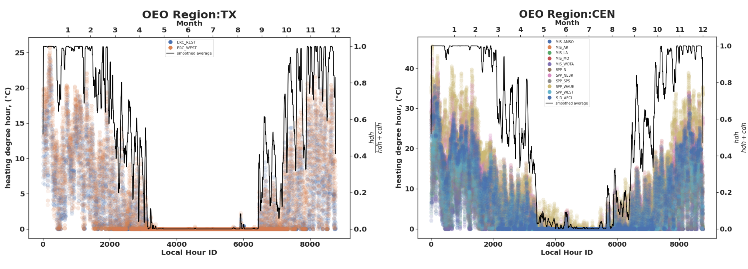
"The raw data from EFS combines space heating and cooling hourly load profiles. To separate the heating and cooling profiles we use population weighted heating and cooling degree hour (hdh/cdh) data provided by Michael Roberts at the University of Hawaii (described in a forthcoming paper). This data is available at the hourly timescale for the year 2010 and is available across the IPM regions. We first calculate an average hdh for IPM regions within a given OEO region (Figure 1) for each hour of 2010. Next, we calculate the hourly hdh fraction as: \n",
"\\begin{equation*}\n",
"\\frac{\\bar{hdh}}{\\bar{hdh} + \\bar{cdh}}\n",
"\\end{equation*}\n",
"where $\\bar{hdh}$ and $\\bar{cdh}$ are the hourly hdh and cdh, respectively, averaged across IPM regions in a given OEO region. These fractions are calculated for each hour in each OEO region. Finally, the combined heating and cooling load from NREL EFS is multiplied by these fractions to estimate the heating load in each hour. The cooling load is similarly estimated as the total load multiplied by the fraction of cooling degree hours over the sum of heating and cooling degree hours. This disaggregation of hourly heating and cooling load is illustrated in Figure 2 for two OEO regions.\n",
"\n",
"\n",
"**Figure 2.** Heating degree hour (hdh) and fraction of heating degree hour for the OEO ‘TX’ (left) and 'CEN' (right) region. The markers on the plot show the hourly hdh for the IPM regions within the given OEO region. The line shows the average hdh fraction for each hour smoothed with a moving average window of 20 hours for legibility."
]
},
{
"cell_type": "code",
"execution_count": 3,
"metadata": {
"hide_input": true,
"init_cell": true
},
"outputs": [
{
"data": {
"text/markdown": [
"The hourly demand profiles for residential/commercial end use demand are shown below."
],
"text/plain": [
""
]
},
"metadata": {},
"output_type": "display_data"
},
{
"data": {
"application/vnd.jupyter.widget-view+json": {
"model_id": "2affa79b96c9411889fe0f04d67a63ec",
"version_major": 2,
"version_minor": 0
},
"text/plain": [
"VBox(children=(HBox(children=(Select(description='region', options=('CA', 'CEN', 'MID_AT', 'NE', 'NW', 'N_CEN'…"
]
},
"metadata": {},
"output_type": "display_data"
}
],
"source": [
"display(Markdown('The hourly demand profiles for residential/commercial end use demand are shown below.'))\n",
"\n",
"def show_hourly_dem(conn):\n",
" df_dds = pd.read_sql_query('SELECT * FROM DemandSpecificDistribution', conn)\n",
" regions = df_dds.regions.unique()\n",
" unique_demands = df_dds.demand_name.unique()\n",
" \n",
" def select_region(region='', dem_name=''):\n",
" df_sel = df_dds.loc[(df_dds.regions==region) & (df_dds.demand_name==dem_name)].copy()\n",
" fig, ax = plt.subplots(figsize=(10,6))\n",
" plt.plot(np.arange(0, len(df_sel['dds'])),df_sel['dds'], label=dem_name)\n",
" plt.ylabel('Hourly demand fraction')\n",
" plt.xlabel('Hour')\n",
" plt.legend(loc='upper right',bbox_to_anchor=(1.2, 1))\n",
"\n",
" w1 = widgets.Select(options=regions)\n",
" w2 = widgets.Select(options=unique_demands)\n",
" w = widgets.interactive(select_region, region=w1, dem_name=w2)\n",
" \n",
" controls_rows(w)\n",
"\n",
"show_hourly_dem(con)"
]
},
{
"cell_type": "markdown",
"metadata": {},
"source": [
"## Demand Technology Specification \n",
"\n",
"The characteristics of the demand technologies in the residential and commercial sectors in the OEO database are based on the Residential Demand Module (RDM) and Commercial Demand Module (CDM) of the National Energy Modeling System (NEMS) - [Updated Buildings Sector Appliance and Equipment Costs and Efficiency](https://www.eia.gov/analysis/studies/buildings/equipcosts/). In our database we incorporate the **1) technology-specific efficiencies**, **2) fixed and variable operations and maintenance costs**, **3) investment costs**, **4) lifetimes**, and 5) **typical capacities** reported in the appendices which are based on contract reports prepared by Navigant Consulting, Inc. for the U.S. Energy Information Administration. In this way we are able to represent a diverse set of equipment classes/types capable of servicing different parts of the buildings sector. For example, the technologies capable of meeting residential cooling demand include room air conditioners, central air conditioners, and heat pumps. Three types of heat pumps are represented for residential cooling: air-source, ground-source, and natural gas heat pumps. We used this dataset as-is, except for an adjustment of the heat pump coefficient of performance (COP) to reflect more regionally appropriate values. [Vaishnav et al. (2020)](https://pubs.acs.org/doi/abs/10.1021/acs.est.0c02705) used a dataset gathered from NEEP and estimated a linear relationship between COP and outside temperature for a variety of heat pumps. Their approach assumed that the indoor temperatures stay constant at 70 F. We use the slope of this linear relationship to adjust heat pump COPs at the OEO region level using the NEMS database and applying state-level population weighted temperatures.\n",
"\n",
"Along with diversity in technology representations, the appendices above project the techno-economic parameters for residential and commercial equipment from 2020 to 2050 in 5 year increments. In most cases, two versions of the same technology for a given vintage are included in our database: 1) a standard version and 2) a high efficiency version. For example: The heating seasonal performance factors (HSPF) for a typical air-source heat pump of a 2020 vintage is 8.6 whereas a high-efficiency version has an HSPF of 9.0 (the costs, lifetimes may also vary across these different versions). These different versions of technologies are utilized as part of the OEO buildings database. The techno-economic parameters are assumed to be region agnostic with the exception of heat pump COPs as described above. \n",
"\n",
"Input values drawn directly from the database can be viewed in the sections below."
]
},
{
"cell_type": "markdown",
"metadata": {},
"source": [
"### Investment costs "
]
},
{
"cell_type": "markdown",
"metadata": {},
"source": [
"The investment costs are drawn from the [Residential Demand Module (RDM) and Commercial Demand Module (CDM)](https://www.eia.gov/analysis/studies/buildings/equipcosts/) of National Energy Modeling System. Specific values can be inspected using the look up tool below."
]
},
{
"cell_type": "code",
"execution_count": 4,
"metadata": {
"hide_input": true,
"init_cell": true,
"jupyter": {
"source_hidden": true
}
},
"outputs": [
{
"data": {
"application/vnd.jupyter.widget-view+json": {
"model_id": "3bf13ed28977479b86f582c2977f52aa",
"version_major": 2,
"version_minor": 0
},
"text/plain": [
"VBox(children=(HBox(children=(Select(description='tech', options=('All', 'high efficiency distillate boiler/ra…"
]
},
"metadata": {},
"output_type": "display_data"
}
],
"source": [
"def show_cost_invest(con):\n",
" \n",
" df_tech_desc = pd.read_sql(\"SELECT tech, tech_desc FROM technologies\", con)\n",
"\n",
" df = pd.read_sql(\n",
" \"SELECT regions, tech,vintage, cost_invest, cost_invest_units FROM CostInvest WHERE tech IN (SELECT tech FROM technologies WHERE sector=='residential' OR sector='commercial' ) ORDER BY tech, vintage\",\n",
" con)\n",
"\n",
" display_types = ['table', 'figure']\n",
" \n",
" df['agg_tech'] = df['tech'].map(lambda x: df_tech_desc.loc[df_tech_desc.tech==x,'tech_desc'].values[0].replace('#','').strip())\n",
" techs = []\n",
" for unique_tech in df.agg_tech.unique():\n",
" try:\n",
" int(unique_tech.split('_')[-1])\n",
" techs.append('_'.join(unique_tech.split('_')[0:-1]))\n",
" except:\n",
" techs.append(unique_tech)\n",
" techs = ['All'] + list(set(techs))\n",
" regions = df.regions.unique()\n",
"\n",
"\n",
" def filter_tech(tech='', region='', o_format=''):\n",
" if tech == 'All':\n",
" df_sel = df[(df.regions == region)]\n",
" else:\n",
" df_sel = df[(df.agg_tech.str.contains(tech, regex=False)) & (df.regions == region)]\n",
" if o_format == 'table':\n",
" df_sel = df_sel.pivot_table(\n",
" index=['regions', 'tech', 'agg_tech', 'cost_invest_units'],\n",
" columns='vintage',\n",
" values='cost_invest').reset_index().set_index('regions')\n",
" df_sel.rename(columns={'cost_invest_units': 'units', 'agg_tech':'description'}, inplace=True)\n",
" df_sel['units'] = df_sel['units'].str.replace('#','').str.replace('M$','$M').str.strip()\n",
" if len(df_sel['units'].unique())==1:\n",
" df_sel['units'] = df_sel['units'].unique()[0].replace('M$','$M')\n",
" display(\n",
" HTML(\n",
" tabulate.tabulate(df_sel,\n",
" ['region'] + list(df_sel.columns.values),\n",
" floatfmt=\".0f\",\n",
" tablefmt='html')))\n",
" elif (o_format == 'figure') & (tech!='All') :\n",
" fig, ax = plt.subplots(figsize=(10, 6))\n",
" for ind_tech in df_sel.tech.unique():\n",
" plt.plot(df_sel[df_sel.tech == ind_tech].vintage,\n",
" df_sel[df_sel.tech == ind_tech].cost_invest,\n",
" label=ind_tech)\n",
" plt.legend()\n",
" plt.ylabel('Investment costs (' + df_sel['cost_invest_units'].unique()[0].replace('#','').strip().replace('M$','$M') + ')')\n",
" #plt.ylim([0, df.cost_invest.max() * 1.1])\n",
" plt.xlabel('Vintage')\n",
"\n",
"\n",
" w1 = widgets.Select(options=techs)\n",
" w2 = widgets.Select(options=regions)\n",
" w3 = widgets.Select(options=display_types)\n",
" w = widgets.interactive(filter_tech, tech=w1, region=w2, o_format=w3)\n",
"\n",
" controls_rows(w)\n",
" \n",
" \n",
" \n",
"show_cost_invest(con)"
]
},
{
"cell_type": "markdown",
"metadata": {},
"source": [
"### Efficiency "
]
},
{
"cell_type": "markdown",
"metadata": {},
"source": [
"Our representation of the buildings sector is comprised of several end-use services like residential space heating and commercial ventilation (listed in Table 1). These end-use service demands are met by a host of demand technologies that consume energy commodities and produce end-use demand commodities. In this section, we consider the numerous efficiency metrics that allow for this conversion and how they are represented in the OEO buildings database.\n",
"\n",
"Table 3 summarizes the end-use service demand, the efficiency metrics of the technologies used to service that demand and the units of the efficiency metric in the OEO database. The demands for some end-use services (like residential space heating) are specified in energy units and so the efficiencies of technologies meeting these demands are in units of energy output over energy input supplied. However, other end-use services (like commercial ventilation) have demand specified in physical units, and thus the efficiencies of the associated demand technologies are in physical units produced over input energy supplied. \n",
"\n",
"**Table 3.** Summary of technology efficiencies applied to building sub-sectors in the OEO database. \n",
"\n",
"| End-Use Demand | Efficiency Metrics | Efficiency Units\n",
"|:-|:-|:-|\n",
"| Commercial Space Cooling
\n",
"\n",
"**Figure 1.** The nine US regions developed for the electric sector in the OEO input database, based on aggregations of IPM regions\n",
"\n",
"The raw data from EFS combines space heating and cooling hourly load profiles. To separate the heating and cooling profiles we use population weighted heating and cooling degree hour (hdh/cdh) data provided by Michael Roberts at the University of Hawaii (described in a forthcoming paper). This data is available at the hourly timescale for the year 2010 and is available across the IPM regions. We first calculate an average hdh for IPM regions within a given OEO region (Figure 1) for each hour of 2010. Next, we calculate the hourly hdh fraction as: \n",
"\\begin{equation*}\n",
"\\frac{\\bar{hdh}}{\\bar{hdh} + \\bar{cdh}}\n",
"\\end{equation*}\n",
"where $\\bar{hdh}$ and $\\bar{cdh}$ are the hourly hdh and cdh, respectively, averaged across IPM regions in a given OEO region. These fractions are calculated for each hour in each OEO region. Finally, the combined heating and cooling load from NREL EFS is multiplied by these fractions to estimate the heating load in each hour. The cooling load is similarly estimated as the total load multiplied by the fraction of cooling degree hours over the sum of heating and cooling degree hours. This disaggregation of hourly heating and cooling load is illustrated in Figure 2 for two OEO regions.\n",
"\n",
"\n",
"**Figure 2.** Heating degree hour (hdh) and fraction of heating degree hour for the OEO ‘TX’ (left) and 'CEN' (right) region. The markers on the plot show the hourly hdh for the IPM regions within the given OEO region. The line shows the average hdh fraction for each hour smoothed with a moving average window of 20 hours for legibility."
]
},
{
"cell_type": "code",
"execution_count": 3,
"metadata": {
"hide_input": true,
"init_cell": true
},
"outputs": [
{
"data": {
"text/markdown": [
"The hourly demand profiles for residential/commercial end use demand are shown below."
],
"text/plain": [
""
]
},
"metadata": {},
"output_type": "display_data"
},
{
"data": {
"application/vnd.jupyter.widget-view+json": {
"model_id": "2affa79b96c9411889fe0f04d67a63ec",
"version_major": 2,
"version_minor": 0
},
"text/plain": [
"VBox(children=(HBox(children=(Select(description='region', options=('CA', 'CEN', 'MID_AT', 'NE', 'NW', 'N_CEN'…"
]
},
"metadata": {},
"output_type": "display_data"
}
],
"source": [
"display(Markdown('The hourly demand profiles for residential/commercial end use demand are shown below.'))\n",
"\n",
"def show_hourly_dem(conn):\n",
" df_dds = pd.read_sql_query('SELECT * FROM DemandSpecificDistribution', conn)\n",
" regions = df_dds.regions.unique()\n",
" unique_demands = df_dds.demand_name.unique()\n",
" \n",
" def select_region(region='', dem_name=''):\n",
" df_sel = df_dds.loc[(df_dds.regions==region) & (df_dds.demand_name==dem_name)].copy()\n",
" fig, ax = plt.subplots(figsize=(10,6))\n",
" plt.plot(np.arange(0, len(df_sel['dds'])),df_sel['dds'], label=dem_name)\n",
" plt.ylabel('Hourly demand fraction')\n",
" plt.xlabel('Hour')\n",
" plt.legend(loc='upper right',bbox_to_anchor=(1.2, 1))\n",
"\n",
" w1 = widgets.Select(options=regions)\n",
" w2 = widgets.Select(options=unique_demands)\n",
" w = widgets.interactive(select_region, region=w1, dem_name=w2)\n",
" \n",
" controls_rows(w)\n",
"\n",
"show_hourly_dem(con)"
]
},
{
"cell_type": "markdown",
"metadata": {},
"source": [
"## Demand Technology Specification \n",
"\n",
"The characteristics of the demand technologies in the residential and commercial sectors in the OEO database are based on the Residential Demand Module (RDM) and Commercial Demand Module (CDM) of the National Energy Modeling System (NEMS) - [Updated Buildings Sector Appliance and Equipment Costs and Efficiency](https://www.eia.gov/analysis/studies/buildings/equipcosts/). In our database we incorporate the **1) technology-specific efficiencies**, **2) fixed and variable operations and maintenance costs**, **3) investment costs**, **4) lifetimes**, and 5) **typical capacities** reported in the appendices which are based on contract reports prepared by Navigant Consulting, Inc. for the U.S. Energy Information Administration. In this way we are able to represent a diverse set of equipment classes/types capable of servicing different parts of the buildings sector. For example, the technologies capable of meeting residential cooling demand include room air conditioners, central air conditioners, and heat pumps. Three types of heat pumps are represented for residential cooling: air-source, ground-source, and natural gas heat pumps. We used this dataset as-is, except for an adjustment of the heat pump coefficient of performance (COP) to reflect more regionally appropriate values. [Vaishnav et al. (2020)](https://pubs.acs.org/doi/abs/10.1021/acs.est.0c02705) used a dataset gathered from NEEP and estimated a linear relationship between COP and outside temperature for a variety of heat pumps. Their approach assumed that the indoor temperatures stay constant at 70 F. We use the slope of this linear relationship to adjust heat pump COPs at the OEO region level using the NEMS database and applying state-level population weighted temperatures.\n",
"\n",
"Along with diversity in technology representations, the appendices above project the techno-economic parameters for residential and commercial equipment from 2020 to 2050 in 5 year increments. In most cases, two versions of the same technology for a given vintage are included in our database: 1) a standard version and 2) a high efficiency version. For example: The heating seasonal performance factors (HSPF) for a typical air-source heat pump of a 2020 vintage is 8.6 whereas a high-efficiency version has an HSPF of 9.0 (the costs, lifetimes may also vary across these different versions). These different versions of technologies are utilized as part of the OEO buildings database. The techno-economic parameters are assumed to be region agnostic with the exception of heat pump COPs as described above. \n",
"\n",
"Input values drawn directly from the database can be viewed in the sections below."
]
},
{
"cell_type": "markdown",
"metadata": {},
"source": [
"### Investment costs "
]
},
{
"cell_type": "markdown",
"metadata": {},
"source": [
"The investment costs are drawn from the [Residential Demand Module (RDM) and Commercial Demand Module (CDM)](https://www.eia.gov/analysis/studies/buildings/equipcosts/) of National Energy Modeling System. Specific values can be inspected using the look up tool below."
]
},
{
"cell_type": "code",
"execution_count": 4,
"metadata": {
"hide_input": true,
"init_cell": true,
"jupyter": {
"source_hidden": true
}
},
"outputs": [
{
"data": {
"application/vnd.jupyter.widget-view+json": {
"model_id": "3bf13ed28977479b86f582c2977f52aa",
"version_major": 2,
"version_minor": 0
},
"text/plain": [
"VBox(children=(HBox(children=(Select(description='tech', options=('All', 'high efficiency distillate boiler/ra…"
]
},
"metadata": {},
"output_type": "display_data"
}
],
"source": [
"def show_cost_invest(con):\n",
" \n",
" df_tech_desc = pd.read_sql(\"SELECT tech, tech_desc FROM technologies\", con)\n",
"\n",
" df = pd.read_sql(\n",
" \"SELECT regions, tech,vintage, cost_invest, cost_invest_units FROM CostInvest WHERE tech IN (SELECT tech FROM technologies WHERE sector=='residential' OR sector='commercial' ) ORDER BY tech, vintage\",\n",
" con)\n",
"\n",
" display_types = ['table', 'figure']\n",
" \n",
" df['agg_tech'] = df['tech'].map(lambda x: df_tech_desc.loc[df_tech_desc.tech==x,'tech_desc'].values[0].replace('#','').strip())\n",
" techs = []\n",
" for unique_tech in df.agg_tech.unique():\n",
" try:\n",
" int(unique_tech.split('_')[-1])\n",
" techs.append('_'.join(unique_tech.split('_')[0:-1]))\n",
" except:\n",
" techs.append(unique_tech)\n",
" techs = ['All'] + list(set(techs))\n",
" regions = df.regions.unique()\n",
"\n",
"\n",
" def filter_tech(tech='', region='', o_format=''):\n",
" if tech == 'All':\n",
" df_sel = df[(df.regions == region)]\n",
" else:\n",
" df_sel = df[(df.agg_tech.str.contains(tech, regex=False)) & (df.regions == region)]\n",
" if o_format == 'table':\n",
" df_sel = df_sel.pivot_table(\n",
" index=['regions', 'tech', 'agg_tech', 'cost_invest_units'],\n",
" columns='vintage',\n",
" values='cost_invest').reset_index().set_index('regions')\n",
" df_sel.rename(columns={'cost_invest_units': 'units', 'agg_tech':'description'}, inplace=True)\n",
" df_sel['units'] = df_sel['units'].str.replace('#','').str.replace('M$','$M').str.strip()\n",
" if len(df_sel['units'].unique())==1:\n",
" df_sel['units'] = df_sel['units'].unique()[0].replace('M$','$M')\n",
" display(\n",
" HTML(\n",
" tabulate.tabulate(df_sel,\n",
" ['region'] + list(df_sel.columns.values),\n",
" floatfmt=\".0f\",\n",
" tablefmt='html')))\n",
" elif (o_format == 'figure') & (tech!='All') :\n",
" fig, ax = plt.subplots(figsize=(10, 6))\n",
" for ind_tech in df_sel.tech.unique():\n",
" plt.plot(df_sel[df_sel.tech == ind_tech].vintage,\n",
" df_sel[df_sel.tech == ind_tech].cost_invest,\n",
" label=ind_tech)\n",
" plt.legend()\n",
" plt.ylabel('Investment costs (' + df_sel['cost_invest_units'].unique()[0].replace('#','').strip().replace('M$','$M') + ')')\n",
" #plt.ylim([0, df.cost_invest.max() * 1.1])\n",
" plt.xlabel('Vintage')\n",
"\n",
"\n",
" w1 = widgets.Select(options=techs)\n",
" w2 = widgets.Select(options=regions)\n",
" w3 = widgets.Select(options=display_types)\n",
" w = widgets.interactive(filter_tech, tech=w1, region=w2, o_format=w3)\n",
"\n",
" controls_rows(w)\n",
" \n",
" \n",
" \n",
"show_cost_invest(con)"
]
},
{
"cell_type": "markdown",
"metadata": {},
"source": [
"### Efficiency "
]
},
{
"cell_type": "markdown",
"metadata": {},
"source": [
"Our representation of the buildings sector is comprised of several end-use services like residential space heating and commercial ventilation (listed in Table 1). These end-use service demands are met by a host of demand technologies that consume energy commodities and produce end-use demand commodities. In this section, we consider the numerous efficiency metrics that allow for this conversion and how they are represented in the OEO buildings database.\n",
"\n",
"Table 3 summarizes the end-use service demand, the efficiency metrics of the technologies used to service that demand and the units of the efficiency metric in the OEO database. The demands for some end-use services (like residential space heating) are specified in energy units and so the efficiencies of technologies meeting these demands are in units of energy output over energy input supplied. However, other end-use services (like commercial ventilation) have demand specified in physical units, and thus the efficiencies of the associated demand technologies are in physical units produced over input energy supplied. \n",
"\n",
"**Table 3.** Summary of technology efficiencies applied to building sub-sectors in the OEO database. \n",
"\n",
"| End-Use Demand | Efficiency Metrics | Efficiency Units\n",
"|:-|:-|:-|\n",
"| Commercial Space Cooling ![]() | COP[1](#COP), EER[2](#EER), IEER[2](#EER)
| COP[1](#COP), EER[2](#EER), IEER[2](#EER) ![]() | PJ-out/PJ-In
| PJ-out/PJ-In![]() |\n",
"| Commercial Cooking | cooking energy efficiency | PJ-out/PJ-In |\n",
"| Commercial Lighting | system efficacy[3](#LIGHT) | Giga-Lumen-Year/PJ |\n",
"| Commercial Refrigeration | Nominal Capacity Over Average Input | PJ-out/PJ-In |\n",
"| Commercial Space Heating | COP, thermal efficiency[4](#TE), COP, AFUE[5](#AFUE)| PJ-out/PJ-In |\n",
"| Commercial Ventilation | ventilation efficiency | Trillion-CFM-hour/PJ-in |\n",
"| Commercial Water Heating | thermal efficiency, SEF[7](#SEF), COP | PJ-out/PJ-In |\n",
"| Residential Space Cooling | SEER[6](#AFUE), EER, COP | PJ-out/PJ-In |\n",
"| Residential Refrigeration | typical capacity over annual energy consumption | Mega-Cubic-Feet/PJ |\n",
"| Residential Lighting | system efficacy | Giga-Lumen-Year/PJ |\n",
"| Residential Space Heating | AFUE, thermal efficiency, HSPF[8](#HSPF), COP, HHV[9](#HHV)| PJ-out/PJ-In |\n",
"| Residential Water Heating | UEF[7](#SEF), SEF[7](#SEF) | PJ-out/PJ-In |\n",
"| Residential Clothes Drying | Combined Energy Factor | Giga-Lb/PJ |\n",
"| Residential Dishwashing | cycles per year over annual energy use | Giga-Cycles/PJ |\n",
"| Residential Freezing | typical capacity over annual energy consumption | Mega-Cubic-Feet/PJ |\n",
"| Residential Cooking | cooking energy efficiency | PJ-out/PJ-in |\n",
"\n",
"1: Coefficient of Performance (COP): Energy efficiency rating measure determined, under specific testing conditions, by dividing the useful heating or cooling delivered by the required energy input.\n",
"2: Energy Efficiency Ratio (EER, IEER): A ratio representing the cooling capacity in Btu per hour by the power input in watts at any given set of rating conditions, expressed in Btu per hour per watt.\n",
"3: Lighting efficiencies are represented by efficacy in lumens/watt.\n",
"4: Thermal efficiency (TE): the percentage of input heat energy that is transformed into useful work.\n",
"5: Annual Fuel Utilization Efficiency (AFUE): Efficiency rating based on average usage, including on and off cycling, as set out in the Department of Energy's standardized test procedures.\n",
"6: Seasonal Energy Efficiency Ratio (SEER): The total cooling of a central unitary air conditioner or a unitary heat pump in Btu during its normal annual usage period for cooling divided by the total electric energy input in watt-hours during the same period. \n",
"7: Solar Energy Factor (SEF) and Uniform Energy Factor (UEF): defined as the energy delivered by the system divided the electrical or gas energy put into the system.\n",
"8: Heating Seasonal Performance Factor (HSPF): The total heating delivered by a heat pump in Btu during its normal annual usage period for heating divided by total electric input in watt-hours during the same period.\n",
"9: Higher Heating Value (HHV): This thermal efficiency is fuel dependent and accounts for the latent heat of vaporization of water in the combustion products.\n",
"\n",
"As noted above, several end-use service demands are defined by units of service rather than energy. In these cases, the specified efficiency has different input and output units:\n",
"\n",
"- **Commercial Lighting**:\n",
"Here conversion from electrical energy to lumens is represented by the system efficacy. The system efficacy is published in $\\frac{Lumens}{Watt}$ and converted to $\\frac{Giga-Lumens\\cdot year}{PJ}$ by multiplying by $ 10^{-9} \\frac{Giga}{1} / (3600 \\frac{J}{Wh} \\times 10^{-15} \\frac{PJ}{J} \\times 8760 \\frac{hours}{year}) $.\n",
"- **Commercial Ventilation**:\n",
"These conversion factors are taken from the Commercial Demand Module of the National Energy Modeling System as $\\frac{Trillion-CFM-hours}{PJ}$\n",
"- **Residential Refrigeration**:\n",
"An efficiency is derived as the typical capacity over annual energy consumption where typical capacity is in units of ft3 and annual energy consumption is in the units of kWh and subsequently converted to $\\frac{ft^3}{PJ}$ by dividing by $ 3.6\\times 10^{-9} \\frac{PJ}{kWh} $.\n",
"- **Residential Lighting**:\n",
"Here conversion from electrical energy to lumens is represented by the system efficacy. The system efficacy is published in $\\frac{Lumens}{Watt}$ and converted to $\\frac{Giga-Lumens\\cdot year}{PJ}$ by multiplying by $ 10^{-9} \\frac{Giga}{1} / (3600 \\frac{J}{Wh} \\times 10^{-15} \\frac{PJ}{J} \\times 8760 \\frac{hours}{year}) $.\n",
"- **Residential Clothes Drying**:\n",
"The combined energy factor in the [EIA appendicies](https://www.eia.gov/analysis/studies/buildings/equipcosts/) are presented in units of $\\frac{lb}{kWh}$ and converted to $\\frac{Giga-lb}{PJ}$ by multiplying by $10^{-9}\\frac{Giga}{1} / (3.6\\times10^{-9}\\frac{PJ}{kWh})$\n",
"- **Residential Dishwashing**:\n",
"An efficiency is derived as the number of cycles in year over the typical annual energy use. An average of 215 cycles/year is assumed as per the [EIA appendicies](https://www.eia.gov/analysis/studies/buildings/equipcosts/). The calculated efficiency is presented in units of $\\frac{cycles}{kWh}$ and converted to $\\frac{Giga-cycles}{PJ}$ by multiplying by $10^{-9}\\frac{Giga}{1} / (3.6\\times10^{-9}\\frac{PJ}{kWh})$\n",
"- **Residential Freezing**:\n",
"An efficiency is derived as the typical capacity over annual energy consumption where typical capacity is in units of ft3 and annual energy consumption is in the units of kWh and subsequently converted to $\\frac{mega ft^3}{PJ}$ by multiplying by $ \\frac{10^{-6}}{3.6\\times 10^{-9}} \\frac{PJ}{kWh} $.\n",
"\n",
"\n",
"To calculate efficiencies for commercial refrigeration technologies, the following approach was adopted:\n",
"- **Commercial Refrigeration**:\n",
"An efficiency is derived as the nominal capacity over average input, calculated as the cooling or heat rejection capacity over the annual energy consumption with units of $\\frac{PJ in}{PJ out}$, where the cooling or heat rejection capacity is in units of $\\frac{Btu}{hour}$ and the annual energy consumption is in units of $\\frac{kWh}{Year}$. The unit conversions are as follows (Note that $\\frac{PJ out}{PJ in} = \\frac{Btu out}{But in}$ since the conversion factors cancel out):\n",
"\\begin{equation*}\n",
"\\frac{Capacity \\frac{Btu}{hour} \\times 24 \\frac{hours}{day} \\times 365 \\frac{day}{year}}{Annual Energy Consumption \\frac{kWh}{Year} \\times 3421.14 \\frac {Btu}{kWh}}\n",
"\\end{equation*}."
]
},
{
"cell_type": "code",
"execution_count": 5,
"metadata": {
"hide_input": true,
"init_cell": true,
"jupyter": {
"source_hidden": true
}
},
"outputs": [
{
"data": {
"application/vnd.jupyter.widget-view+json": {
"model_id": "af73353f751d4f88920984fb9c8ff9f5",
"version_major": 2,
"version_minor": 0
},
"text/plain": [
"VBox(children=(HBox(children=(Select(description='tech', options=('All', 'high efficiency range, electric-indu…"
]
},
"metadata": {},
"output_type": "display_data"
}
],
"source": [
"def show_efficiency(con):\n",
" df_tech_desc = pd.read_sql(\"SELECT tech, tech_desc FROM technologies\", con)\n",
" df = pd.read_sql(\"SELECT regions, tech, vintage, efficiency, eff_notes FROM Efficiency WHERE tech IN (SELECT tech FROM technologies WHERE sector=='residential' OR sector='commercial')\", con)\n",
" df.loc[:,'agg_tech'] = df.loc[:,'tech'] #[map_plants[y] for x in df.tech for y in map_plants.keys() if y.lower() in x.lower()] #map agg technologies\n",
" df_sum = df#df.drop(\"vintage\", axis=1).groupby(by = ['regions','agg_tech']).sum().reset_index()\n",
" df_sum['agg_tech'] = df_sum['agg_tech'].map(lambda x: df_tech_desc.loc[df_tech_desc.tech==x,'tech_desc'].values[0].replace('#','').strip())\n",
" techs = ['All'] + list(df_sum.agg_tech.unique())\n",
" regions = df_sum.regions.unique()\n",
" def filter_tech(tech ='', region = ''):\n",
" if tech=='All':\n",
" df_sel = df_sum[(df_sum.regions==region)]\n",
" else:\n",
" df_sel = df_sum[(df_sum.agg_tech==tech) & (df_sum.regions==region)]\n",
"# df_sel.efficiency = 100*df_sel.efficiency\n",
" df_sel = df_sel[['regions','tech','agg_tech','vintage','efficiency', 'eff_notes']]\n",
" display(HTML(tabulate.tabulate(df_sel.set_index('regions'), [\"regions\", \"technology\", \"description\",\"vintage\",'efficiency', 'efficiency units' ], floatfmt=\".1f\", tablefmt='html')))\n",
"\n",
" w1 = widgets.Select(options=techs)\n",
" w2 = widgets.Select(options=regions)\n",
" w = widgets.interactive(filter_tech, tech=w1, region=w2)\n",
"\n",
" controls_rows(w)\n",
" \n",
"show_efficiency(con)"
]
},
{
"cell_type": "markdown",
"metadata": {},
"source": [
"### Existing Capacity "
]
},
{
"cell_type": "markdown",
"metadata": {},
"source": [
"To our knowledge, the existing installed capacities of the various technologies listed in the [EIA dataset](https://www.eia.gov/analysis/studies/buildings/equipcosts/) are not readily available. Here we rely on two main data source to estimate existing capacity at the technology level for each sub-sector in the OEO buildings database: **1) NREL EFS service demands scaled using a derived utilization factor** and **2) USEPA9r MARKAL database**. Table 3 provides a summary of which data sources are used for each of the represented sub-sectors.\n",
"\n",
"**Table 3.** Summary of data sources used to estimate existing installed capacity for the buildings sub-sectors in the OEO database. \n",
"\n",
"| End-Use Demand | Data Source |\n",
"|:-|:-|\n",
"| Commercial Space Cooling
|\n",
"| Commercial Cooking | cooking energy efficiency | PJ-out/PJ-In |\n",
"| Commercial Lighting | system efficacy[3](#LIGHT) | Giga-Lumen-Year/PJ |\n",
"| Commercial Refrigeration | Nominal Capacity Over Average Input | PJ-out/PJ-In |\n",
"| Commercial Space Heating | COP, thermal efficiency[4](#TE), COP, AFUE[5](#AFUE)| PJ-out/PJ-In |\n",
"| Commercial Ventilation | ventilation efficiency | Trillion-CFM-hour/PJ-in |\n",
"| Commercial Water Heating | thermal efficiency, SEF[7](#SEF), COP | PJ-out/PJ-In |\n",
"| Residential Space Cooling | SEER[6](#AFUE), EER, COP | PJ-out/PJ-In |\n",
"| Residential Refrigeration | typical capacity over annual energy consumption | Mega-Cubic-Feet/PJ |\n",
"| Residential Lighting | system efficacy | Giga-Lumen-Year/PJ |\n",
"| Residential Space Heating | AFUE, thermal efficiency, HSPF[8](#HSPF), COP, HHV[9](#HHV)| PJ-out/PJ-In |\n",
"| Residential Water Heating | UEF[7](#SEF), SEF[7](#SEF) | PJ-out/PJ-In |\n",
"| Residential Clothes Drying | Combined Energy Factor | Giga-Lb/PJ |\n",
"| Residential Dishwashing | cycles per year over annual energy use | Giga-Cycles/PJ |\n",
"| Residential Freezing | typical capacity over annual energy consumption | Mega-Cubic-Feet/PJ |\n",
"| Residential Cooking | cooking energy efficiency | PJ-out/PJ-in |\n",
"\n",
"1: Coefficient of Performance (COP): Energy efficiency rating measure determined, under specific testing conditions, by dividing the useful heating or cooling delivered by the required energy input.\n",
"2: Energy Efficiency Ratio (EER, IEER): A ratio representing the cooling capacity in Btu per hour by the power input in watts at any given set of rating conditions, expressed in Btu per hour per watt.\n",
"3: Lighting efficiencies are represented by efficacy in lumens/watt.\n",
"4: Thermal efficiency (TE): the percentage of input heat energy that is transformed into useful work.\n",
"5: Annual Fuel Utilization Efficiency (AFUE): Efficiency rating based on average usage, including on and off cycling, as set out in the Department of Energy's standardized test procedures.\n",
"6: Seasonal Energy Efficiency Ratio (SEER): The total cooling of a central unitary air conditioner or a unitary heat pump in Btu during its normal annual usage period for cooling divided by the total electric energy input in watt-hours during the same period. \n",
"7: Solar Energy Factor (SEF) and Uniform Energy Factor (UEF): defined as the energy delivered by the system divided the electrical or gas energy put into the system.\n",
"8: Heating Seasonal Performance Factor (HSPF): The total heating delivered by a heat pump in Btu during its normal annual usage period for heating divided by total electric input in watt-hours during the same period.\n",
"9: Higher Heating Value (HHV): This thermal efficiency is fuel dependent and accounts for the latent heat of vaporization of water in the combustion products.\n",
"\n",
"As noted above, several end-use service demands are defined by units of service rather than energy. In these cases, the specified efficiency has different input and output units:\n",
"\n",
"- **Commercial Lighting**:\n",
"Here conversion from electrical energy to lumens is represented by the system efficacy. The system efficacy is published in $\\frac{Lumens}{Watt}$ and converted to $\\frac{Giga-Lumens\\cdot year}{PJ}$ by multiplying by $ 10^{-9} \\frac{Giga}{1} / (3600 \\frac{J}{Wh} \\times 10^{-15} \\frac{PJ}{J} \\times 8760 \\frac{hours}{year}) $.\n",
"- **Commercial Ventilation**:\n",
"These conversion factors are taken from the Commercial Demand Module of the National Energy Modeling System as $\\frac{Trillion-CFM-hours}{PJ}$\n",
"- **Residential Refrigeration**:\n",
"An efficiency is derived as the typical capacity over annual energy consumption where typical capacity is in units of ft3 and annual energy consumption is in the units of kWh and subsequently converted to $\\frac{ft^3}{PJ}$ by dividing by $ 3.6\\times 10^{-9} \\frac{PJ}{kWh} $.\n",
"- **Residential Lighting**:\n",
"Here conversion from electrical energy to lumens is represented by the system efficacy. The system efficacy is published in $\\frac{Lumens}{Watt}$ and converted to $\\frac{Giga-Lumens\\cdot year}{PJ}$ by multiplying by $ 10^{-9} \\frac{Giga}{1} / (3600 \\frac{J}{Wh} \\times 10^{-15} \\frac{PJ}{J} \\times 8760 \\frac{hours}{year}) $.\n",
"- **Residential Clothes Drying**:\n",
"The combined energy factor in the [EIA appendicies](https://www.eia.gov/analysis/studies/buildings/equipcosts/) are presented in units of $\\frac{lb}{kWh}$ and converted to $\\frac{Giga-lb}{PJ}$ by multiplying by $10^{-9}\\frac{Giga}{1} / (3.6\\times10^{-9}\\frac{PJ}{kWh})$\n",
"- **Residential Dishwashing**:\n",
"An efficiency is derived as the number of cycles in year over the typical annual energy use. An average of 215 cycles/year is assumed as per the [EIA appendicies](https://www.eia.gov/analysis/studies/buildings/equipcosts/). The calculated efficiency is presented in units of $\\frac{cycles}{kWh}$ and converted to $\\frac{Giga-cycles}{PJ}$ by multiplying by $10^{-9}\\frac{Giga}{1} / (3.6\\times10^{-9}\\frac{PJ}{kWh})$\n",
"- **Residential Freezing**:\n",
"An efficiency is derived as the typical capacity over annual energy consumption where typical capacity is in units of ft3 and annual energy consumption is in the units of kWh and subsequently converted to $\\frac{mega ft^3}{PJ}$ by multiplying by $ \\frac{10^{-6}}{3.6\\times 10^{-9}} \\frac{PJ}{kWh} $.\n",
"\n",
"\n",
"To calculate efficiencies for commercial refrigeration technologies, the following approach was adopted:\n",
"- **Commercial Refrigeration**:\n",
"An efficiency is derived as the nominal capacity over average input, calculated as the cooling or heat rejection capacity over the annual energy consumption with units of $\\frac{PJ in}{PJ out}$, where the cooling or heat rejection capacity is in units of $\\frac{Btu}{hour}$ and the annual energy consumption is in units of $\\frac{kWh}{Year}$. The unit conversions are as follows (Note that $\\frac{PJ out}{PJ in} = \\frac{Btu out}{But in}$ since the conversion factors cancel out):\n",
"\\begin{equation*}\n",
"\\frac{Capacity \\frac{Btu}{hour} \\times 24 \\frac{hours}{day} \\times 365 \\frac{day}{year}}{Annual Energy Consumption \\frac{kWh}{Year} \\times 3421.14 \\frac {Btu}{kWh}}\n",
"\\end{equation*}."
]
},
{
"cell_type": "code",
"execution_count": 5,
"metadata": {
"hide_input": true,
"init_cell": true,
"jupyter": {
"source_hidden": true
}
},
"outputs": [
{
"data": {
"application/vnd.jupyter.widget-view+json": {
"model_id": "af73353f751d4f88920984fb9c8ff9f5",
"version_major": 2,
"version_minor": 0
},
"text/plain": [
"VBox(children=(HBox(children=(Select(description='tech', options=('All', 'high efficiency range, electric-indu…"
]
},
"metadata": {},
"output_type": "display_data"
}
],
"source": [
"def show_efficiency(con):\n",
" df_tech_desc = pd.read_sql(\"SELECT tech, tech_desc FROM technologies\", con)\n",
" df = pd.read_sql(\"SELECT regions, tech, vintage, efficiency, eff_notes FROM Efficiency WHERE tech IN (SELECT tech FROM technologies WHERE sector=='residential' OR sector='commercial')\", con)\n",
" df.loc[:,'agg_tech'] = df.loc[:,'tech'] #[map_plants[y] for x in df.tech for y in map_plants.keys() if y.lower() in x.lower()] #map agg technologies\n",
" df_sum = df#df.drop(\"vintage\", axis=1).groupby(by = ['regions','agg_tech']).sum().reset_index()\n",
" df_sum['agg_tech'] = df_sum['agg_tech'].map(lambda x: df_tech_desc.loc[df_tech_desc.tech==x,'tech_desc'].values[0].replace('#','').strip())\n",
" techs = ['All'] + list(df_sum.agg_tech.unique())\n",
" regions = df_sum.regions.unique()\n",
" def filter_tech(tech ='', region = ''):\n",
" if tech=='All':\n",
" df_sel = df_sum[(df_sum.regions==region)]\n",
" else:\n",
" df_sel = df_sum[(df_sum.agg_tech==tech) & (df_sum.regions==region)]\n",
"# df_sel.efficiency = 100*df_sel.efficiency\n",
" df_sel = df_sel[['regions','tech','agg_tech','vintage','efficiency', 'eff_notes']]\n",
" display(HTML(tabulate.tabulate(df_sel.set_index('regions'), [\"regions\", \"technology\", \"description\",\"vintage\",'efficiency', 'efficiency units' ], floatfmt=\".1f\", tablefmt='html')))\n",
"\n",
" w1 = widgets.Select(options=techs)\n",
" w2 = widgets.Select(options=regions)\n",
" w = widgets.interactive(filter_tech, tech=w1, region=w2)\n",
"\n",
" controls_rows(w)\n",
" \n",
"show_efficiency(con)"
]
},
{
"cell_type": "markdown",
"metadata": {},
"source": [
"### Existing Capacity "
]
},
{
"cell_type": "markdown",
"metadata": {},
"source": [
"To our knowledge, the existing installed capacities of the various technologies listed in the [EIA dataset](https://www.eia.gov/analysis/studies/buildings/equipcosts/) are not readily available. Here we rely on two main data source to estimate existing capacity at the technology level for each sub-sector in the OEO buildings database: **1) NREL EFS service demands scaled using a derived utilization factor** and **2) USEPA9r MARKAL database**. Table 3 provides a summary of which data sources are used for each of the represented sub-sectors.\n",
"\n",
"**Table 3.** Summary of data sources used to estimate existing installed capacity for the buildings sub-sectors in the OEO database. \n",
"\n",
"| End-Use Demand | Data Source |\n",
"|:-|:-|\n",
"| Commercial Space Cooling ![]() | NREL EFS[1](#EFS)
| NREL EFS[1](#EFS) ![]() | \n",
"| Commercial Cooking | NREL EFS | \n",
"| Commercial Lighting | EPA MARKAL[2](#MARKAL) | \n",
"| Commercial Refrigeration | NREL EFS | \n",
"| Commercial Space Heating | NREL EFS | \n",
"| Commercial Ventilation | EPA MARKAL | \n",
"| Commercial Water Heating | NREL EFS | \n",
"| Residential Space Cooling | NREL EFS | \n",
"| Residential Refrigeration | NREL EFS | \n",
"| Residential Lighting | EPA MARKAL | \n",
"| Residential Space Heating | NREL EFS | \n",
"| Residential Water Heating | EPA MARKAL | \n",
"| Residential Clothes Drying | NREL EFS | \n",
"| Residential Dishwashing | NREL EFS | \n",
"| Residential Freezing | NREL EFS | \n",
"| Residential Cooking | NREL EFS |\n",
"\n",
"1: [NREL Electrification Futures Study (EFS)](https://www.nrel.gov/docs/fy18osti/71500.pdf).\n",
"2: [USEPA9r MARKAL database (Shay et al. 2013)](https://cfpub.epa.gov/si/si_public_record_Report.cfm?Lab=NRMRL&dirEntryID=150883)\n",
"\n",
"The estimation method from the two data sources are briefly described below:\n",
"\n",
"**1) NREL Electrification Futures Study**: First an end-use service demand specific 'utilization factor' is calculated using the hourly load profile data published in the EFS. This is done by calculating the average demand across the 8760 hours divided by the 95th percentile demand for each end-use service demand in each OEO region for which hourly load profiles are available. The existing capacity of the builings sector technologies is then estimated as the service demand in 2017 from EFS scaled using the calculated utilization factors.\n",
"\n",
"**2) USEPA9r MARKAL database**: Here we lean on existing capacity estimations from the USEPA9r MARKAL database [(Shay et al. 2013)](https://cfpub.epa.gov/si/si_public_record_Report.cfm?Lab=NRMRL&dirEntryID=150883). MARKAL spreadsheets report the existing capacities for most of the technologies listed in the EIA dataset for the [nine Census Divisions](https://www2.census.gov/geo/pdfs/maps-data/maps/reference/us_regdiv.pdf). However, since the OEO regions differ from the Census Divisions, we scale the reported existing capacities using [U.S. Census state population data](https://www.census.gov/data/tables/time-series/demo/popest/2010s-state-total.html) to obtain estimates of existing capacity in each U.S. state. Finally, we aggregate up to the OEO regions and estimate the existing capacity of the EIA technologies. \n",
"\n",
"MARKAL estimates the existing capacity by multiplying the demand met (taken from the [AEO](https://www.eia.gov/outlooks/aeo/)) in an end-use service sub-sector by the estimated market share of a technology contributing to the end-use service category. This value is then divided by a utilization factor to estimate existing capacity of a certain technology in a given region. We directly use the calculated existing capacities in the OEO databases for the end-use demands as listed in Table 3."
]
},
{
"cell_type": "code",
"execution_count": 6,
"metadata": {
"hide_input": true,
"init_cell": true,
"jupyter": {
"source_hidden": true
},
"scrolled": true
},
"outputs": [
{
"data": {
"application/vnd.jupyter.widget-view+json": {
"model_id": "a0a968f7d258487f8d03e64fd3f1e3fb",
"version_major": 2,
"version_minor": 0
},
"text/plain": [
"VBox(children=(HBox(children=(Select(description='tech', options=('All', 'existing natural gas furnace for spa…"
]
},
"metadata": {},
"output_type": "display_data"
}
],
"source": [
"def show_exist_cap(con):\n",
" df_tech_desc = pd.read_sql(\"SELECT tech, tech_desc FROM technologies\", con)\n",
" df = pd.read_sql(\"SELECT regions, tech,vintage, exist_cap, exist_cap_units FROM ExistingCapacity WHERE tech IN (SELECT tech FROM technologies WHERE sector=='residential' OR sector='commercial')\", con)\n",
" df.loc[:,'agg_tech'] = df.loc[:,'tech'] #[map_plants[y] for x in df.tech for y in map_plants.keys() if y.lower() in x.lower()] #map agg technologies\n",
" df_sum = df.drop(\"vintage\", axis=1).groupby(by = ['regions','tech','agg_tech','exist_cap_units']).sum().reset_index()\n",
" df_sum.sort_values(by='exist_cap', ascending=False, inplace=True)\n",
" df_sum['agg_tech'] = df_sum['agg_tech'].map(lambda x: df_tech_desc.loc[df_tech_desc.tech==x,'tech_desc'].values[0].replace('#','').strip())\n",
"\n",
" df_sum[['exist_cap_units']] = 'to be updated' # this line needs to be deleted once the units for existing capacity have been updated directly in the database\n",
" \n",
" techs = ['All'] + list(df_sum.agg_tech.unique())\n",
" regions = df_sum.regions.unique()\n",
" def filter_tech(tech ='', region = ''):\n",
" if tech=='All':\n",
" df_sel = df_sum[(df_sum.regions==region)]\n",
" else:\n",
" df_sel = df_sum[(df_sum.agg_tech==tech) & (df_sum.regions==region)]\n",
" display(HTML(tabulate.tabulate(df_sel.set_index('regions'), [\"regions\", \"technology\", \"description\", \"units\",\"capacity\" ], floatfmt=\".1f\", tablefmt='html')))\n",
" w1 = widgets.Select(options=techs)\n",
" w2 = widgets.Select(options=regions)\n",
" w = widgets.interactive(filter_tech, tech=w1, region=w2)\n",
"\n",
" controls_rows(w)\n",
" \n",
"show_exist_cap(con)\n"
]
},
{
"cell_type": "markdown",
"metadata": {
"jupyter": {
"source_hidden": false
}
},
"source": [
"### Discount Rate \n",
"All new capacity is given a technology-specific discount rate of 30%. Without this specification, TEMOA's least cost optimization results in the early replacement of virtually all existing demand technologies with new capacity at higher efficiency. This 30% discount rate is used to ensure that existing capacity is utilized for the remainder of its lifetime under base case assumptions. In the future, we plan to update this hurdle rate based on calibrations from the updated OEO database."
]
},
{
"cell_type": "code",
"execution_count": 7,
"metadata": {
"hide_input": true,
"init_cell": true,
"jupyter": {
"source_hidden": true
},
"scrolled": true
},
"outputs": [
{
"data": {
"application/vnd.jupyter.widget-view+json": {
"model_id": "e79d9b665e5c4fc48a7c25524c01a811",
"version_major": 2,
"version_minor": 0
},
"text/plain": [
"VBox(children=(HBox(children=(Select(description='tech', options=('All', 'high efficiency distillate boiler/ra…"
]
},
"metadata": {},
"output_type": "display_data"
}
],
"source": [
"def show_disc_rate(con):\n",
" df_tech_desc = pd.read_sql(\"SELECT tech, tech_desc FROM technologies\", con)\n",
" df = pd.read_sql(\"SELECT regions, tech, vintage, tech_rate FROM DiscountRate \\\n",
" WHERE tech in (SELECT tech FROM technologies WHERE sector='residential' OR sector='commercial')\", con)\n",
" df['agg_tech'] = df['tech'].map(lambda x: df_tech_desc.loc[df_tech_desc.tech==x,'tech_desc'].values[0].replace('#','').strip())\n",
" techs = []\n",
" for unique_tech in df.agg_tech.unique():\n",
" techs.append(unique_tech)\n",
" techs = ['All'] + list(set(techs))\n",
" regions = df.regions.unique()\n",
" def filter_tech(tech='', region =''):\n",
" if tech=='All':\n",
" df_sel = df[(df.regions==region)]\n",
" else:\n",
" df_sel = df[(df.agg_tech==tech) & (df.regions==region)]\n",
" df_sel = df_sel.pivot_table(index=['regions','tech', 'agg_tech'], columns='vintage', values='tech_rate').reset_index()\n",
" df_sel.rename(columns={'agg_tech':'description'},inplace=True)\n",
" header = list(df_sel.columns.values)\n",
" display(HTML(tabulate.tabulate(df_sel.set_index('regions'), header, floatfmt=\".3f\", tablefmt='html')))\n",
" w1 = widgets.Select(options=techs)\n",
" w2 = widgets.Select(options=regions)\n",
" w = widgets.interactive(filter_tech, tech=w1, region=w2)\n",
"\n",
" controls_rows(w)\n",
" \n",
"show_disc_rate(con)"
]
},
{
"cell_type": "markdown",
"metadata": {},
"source": [
"### Tech Input Split "
]
},
{
"cell_type": "markdown",
"metadata": {},
"source": [
"We specify minimum shares of commodity inputs to residential space heating, commerical space heating, commercial ventilation and commercial refrigeration in the 2020 time period to match historical demand. The shares are determined using 2020 service demand data from NREL EFS. These constraints are lifted for all future time periods in the model allowing it to make decisions on technology adoption."
]
},
{
"cell_type": "markdown",
"metadata": {},
"source": [
"## Look-up Tools "
]
},
{
"cell_type": "markdown",
"metadata": {},
"source": [
"### Technology/Commodity Description Look-up Tool \n",
"Use the tool below to search for any key words that may describe a technology or commodity of interest (e.g. heating, cooling). The tool provides a list of all the technologies in the database that may be relevant to the query."
]
},
{
"cell_type": "code",
"execution_count": 8,
"metadata": {
"hide_input": true,
"init_cell": true,
"jupyter": {
"source_hidden": true
}
},
"outputs": [
{
"data": {
"application/vnd.jupyter.widget-view+json": {
"model_id": "da05d488416440aa966aab61cb14660b",
"version_major": 2,
"version_minor": 0
},
"text/plain": [
"Text(value='space heating demand')"
]
},
"metadata": {},
"output_type": "display_data"
},
{
"data": {
"application/vnd.jupyter.widget-view+json": {
"model_id": "dfe83599a9e94bf7bea061ddb1f02007",
"version_major": 2,
"version_minor": 0
},
"text/plain": [
"Output()"
]
},
"metadata": {},
"output_type": "display_data"
}
],
"source": [
"w = widgets.Text(value='space heating demand')\n",
"display(w)\n",
"def f(w):\n",
" if len(w)>0:\n",
" df1 = pd.read_sql(\"SELECT * FROM commodities WHERE comm_desc LIKE '%\" + w + \"%'\", con)\n",
" df1['desc'] = df1['comm_desc'].str.replace('#','').str.strip()\n",
" df1['comm_tech'] = df1['comm_name']\n",
" df1['type'] = 'commodity'\n",
"\n",
" df2 = pd.read_sql(\"SELECT * FROM technologies WHERE tech_desc LIKE '%\" + w + \"%'\", con)\n",
" df2['desc'] = df2['tech_desc'].str.replace('#','').str.strip()\n",
" df2['comm_tech'] = df2['tech']\n",
" df2['type'] = 'technology'\n",
"\n",
"\n",
" df = pd.concat([df1[['comm_tech','type','desc']], df2[['comm_tech','type','desc']]])\n",
" \n",
" if len(df)>0:\n",
" display(HTML(tabulate.tabulate(df.set_index('comm_tech'),['technology/commodity','type','description'],tablefmt='html')))\n",
" else:\n",
" print('')\n",
" else:\n",
" print('')\n",
" \n",
"\n",
"\n",
"out = widgets.interactive_output(f, {'w': w})\n",
"display(out)"
]
},
{
"cell_type": "markdown",
"metadata": {},
"source": [
"### Network Diagram Look-up Tool \n",
"Use the [description lookup tool](#description_look_up) above to identify specific commodity or technology names. Type the name in the box below to generate a corresponding network diagram for that commodity or technology. The slider can be used to view different upstream levels of the network diagram."
]
},
{
"cell_type": "code",
"execution_count": 9,
"metadata": {
"hide_input": true,
"init_cell": true,
"jupyter": {
"source_hidden": true
}
},
"outputs": [
{
"data": {
"application/vnd.jupyter.widget-view+json": {
"model_id": "033f6647f4f94026a098716de69f6339",
"version_major": 2,
"version_minor": 0
},
"text/plain": [
"Text(value='RSH')"
]
},
"metadata": {},
"output_type": "display_data"
},
{
"data": {
"application/vnd.jupyter.widget-view+json": {
"model_id": "b1ab8f03228f43f5988d891a4fdb99ec",
"version_major": 2,
"version_minor": 0
},
"text/plain": [
"Output()"
]
},
"metadata": {},
"output_type": "display_data"
}
],
"source": [
"w = widgets.Text(value='RSH')\n",
"display(w)\n",
"def f(w):\n",
" if len(w)>0:\n",
" \n",
" df1 = pd.read_sql(\"SELECT comm_name, comm_desc FROM commodities WHERE comm_name='\" + w + \"'\", con)\n",
" df1['desc'] = df1['comm_desc'].str.replace('#','').str.strip()\n",
" df1['comm_tech'] = df1['comm_name']\n",
" df1['type'] = 'commodity'\n",
"\n",
" df2 = pd.read_sql(\"SELECT * FROM technologies WHERE tech='\" + w + \"'\", con)\n",
" df2['desc'] = df2['tech_desc'].str.replace('#','').str.strip()\n",
" df2['comm_tech'] = df2['tech']\n",
" df2['type'] = 'technology'\n",
"\n",
" df = pd.concat([df1[['comm_tech','type','desc']], df2[['comm_tech','type','desc']]])\n",
"\n",
" \n",
" if len(df)>0:\n",
" def show_desc(level):\n",
" display(Markdown(df['desc'][0]))\n",
" final_dem = df['comm_tech'][0]\n",
" df_graph = return_flowd_table(final_dem,level)\n",
" args = create_args_flowd(df_graph)\n",
" colors, quick_run_dot_fmt = return_format_colors()\n",
" args.update(colors)\n",
" #o_str = 'rankdir = \"LR\" ;'\n",
" #r_str = 'rankdir = \"LR\" ; \\n\\t size=\"12,12\";'\n",
" #quick_run_dot_fmt = quick_run_dot_fmt.replace(o_str, r_str)\n",
" dot_graph = quick_run_dot_fmt % args\n",
" display(graphviz.Source(dot_graph))\n",
" w2 = widgets.IntSlider(value=1,min=0,max=10,step=1,description='Level:',disabled=False,continuous_update=True,orientation='horizontal',readout=True,readout_format='d')\n",
" w = widgets.interactive(show_desc, level=w2)\n",
" controls_rows(w)\n",
" else:\n",
" print('')\n",
"\n",
" else:\n",
" print('')\n",
" \n",
"\n",
"\n",
"out = widgets.interactive_output(f, {'w': w})\n",
"display(out)"
]
},
{
"cell_type": "markdown",
"metadata": {},
"source": [
"### Technology/Commodity Look-up Tool \n",
"Use the tool below to retrieve the description for any technology or commodity within the database. Type the commodity or technology name in the box below to view the description. Note that names are case sensitive."
]
},
{
"cell_type": "code",
"execution_count": 10,
"metadata": {
"hide_input": true,
"init_cell": true,
"jupyter": {
"source_hidden": true
}
},
"outputs": [
{
"data": {
"application/vnd.jupyter.widget-view+json": {
"model_id": "057db377e86141d4828adf6a5975e98e",
"version_major": 2,
"version_minor": 0
},
"text/plain": [
"Text(value='RSH')"
]
},
"metadata": {},
"output_type": "display_data"
},
{
"data": {
"application/vnd.jupyter.widget-view+json": {
"model_id": "811dbca5962843fb8c6cfea6a28e3e61",
"version_major": 2,
"version_minor": 0
},
"text/plain": [
"Output()"
]
},
"metadata": {},
"output_type": "display_data"
}
],
"source": [
"w = widgets.Text(value='RSH')\n",
"display(w)\n",
"def f(w):\n",
" df = pd.read_sql(\"SELECT * FROM commodities WHERE comm_name='\" + w + \"'\", con)\n",
" if len(df)==0:\n",
" df = pd.read_sql(\"SELECT * FROM technologies WHERE tech='\" + w + \"'\", con)\n",
"\n",
" if len(df)>0:\n",
" try:\n",
" display(Markdown((df['comm_desc'].values[0].replace('#', '').strip())))\n",
" except:\n",
" display(Markdown(df['tech_desc'].values[0].replace('#', '').strip()))\n",
" else:\n",
" print('')\n",
"\n",
"\n",
"out = widgets.interactive_output(f, {'w': w})\n",
"display(out)\n"
]
}
],
"metadata": {
"celltoolbar": "Initialization Cell",
"hide_input": true,
"kernelspec": {
"display_name": "Python 3 (ipykernel)",
"language": "python",
"name": "python3"
},
"language_info": {
"codemirror_mode": {
"name": "ipython",
"version": 3
},
"file_extension": ".py",
"mimetype": "text/x-python",
"name": "python",
"nbconvert_exporter": "python",
"pygments_lexer": "ipython3",
"version": "3.7.3"
},
"toc": {
"base_numbering": 1,
"nav_menu": {},
"number_sections": true,
"sideBar": true,
"skip_h1_title": false,
"title_cell": "Table of Contents",
"title_sidebar": "Contents",
"toc_cell": false,
"toc_position": {
"height": "calc(100% - 180px)",
"left": "10px",
"top": "150px",
"width": "369.6px"
},
"toc_section_display": true,
"toc_window_display": true
},
"varInspector": {
"cols": {
"lenName": 16,
"lenType": 16,
"lenVar": 40
},
"kernels_config": {
"python": {
"delete_cmd_postfix": "",
"delete_cmd_prefix": "del ",
"library": "var_list.py",
"varRefreshCmd": "print(var_dic_list())"
},
"r": {
"delete_cmd_postfix": ") ",
"delete_cmd_prefix": "rm(",
"library": "var_list.r",
"varRefreshCmd": "cat(var_dic_list()) "
}
},
"types_to_exclude": [
"module",
"function",
"builtin_function_or_method",
"instance",
"_Feature"
],
"window_display": false
}
},
"nbformat": 4,
"nbformat_minor": 4
}
| \n",
"| Commercial Cooking | NREL EFS | \n",
"| Commercial Lighting | EPA MARKAL[2](#MARKAL) | \n",
"| Commercial Refrigeration | NREL EFS | \n",
"| Commercial Space Heating | NREL EFS | \n",
"| Commercial Ventilation | EPA MARKAL | \n",
"| Commercial Water Heating | NREL EFS | \n",
"| Residential Space Cooling | NREL EFS | \n",
"| Residential Refrigeration | NREL EFS | \n",
"| Residential Lighting | EPA MARKAL | \n",
"| Residential Space Heating | NREL EFS | \n",
"| Residential Water Heating | EPA MARKAL | \n",
"| Residential Clothes Drying | NREL EFS | \n",
"| Residential Dishwashing | NREL EFS | \n",
"| Residential Freezing | NREL EFS | \n",
"| Residential Cooking | NREL EFS |\n",
"\n",
"1: [NREL Electrification Futures Study (EFS)](https://www.nrel.gov/docs/fy18osti/71500.pdf).\n",
"2: [USEPA9r MARKAL database (Shay et al. 2013)](https://cfpub.epa.gov/si/si_public_record_Report.cfm?Lab=NRMRL&dirEntryID=150883)\n",
"\n",
"The estimation method from the two data sources are briefly described below:\n",
"\n",
"**1) NREL Electrification Futures Study**: First an end-use service demand specific 'utilization factor' is calculated using the hourly load profile data published in the EFS. This is done by calculating the average demand across the 8760 hours divided by the 95th percentile demand for each end-use service demand in each OEO region for which hourly load profiles are available. The existing capacity of the builings sector technologies is then estimated as the service demand in 2017 from EFS scaled using the calculated utilization factors.\n",
"\n",
"**2) USEPA9r MARKAL database**: Here we lean on existing capacity estimations from the USEPA9r MARKAL database [(Shay et al. 2013)](https://cfpub.epa.gov/si/si_public_record_Report.cfm?Lab=NRMRL&dirEntryID=150883). MARKAL spreadsheets report the existing capacities for most of the technologies listed in the EIA dataset for the [nine Census Divisions](https://www2.census.gov/geo/pdfs/maps-data/maps/reference/us_regdiv.pdf). However, since the OEO regions differ from the Census Divisions, we scale the reported existing capacities using [U.S. Census state population data](https://www.census.gov/data/tables/time-series/demo/popest/2010s-state-total.html) to obtain estimates of existing capacity in each U.S. state. Finally, we aggregate up to the OEO regions and estimate the existing capacity of the EIA technologies. \n",
"\n",
"MARKAL estimates the existing capacity by multiplying the demand met (taken from the [AEO](https://www.eia.gov/outlooks/aeo/)) in an end-use service sub-sector by the estimated market share of a technology contributing to the end-use service category. This value is then divided by a utilization factor to estimate existing capacity of a certain technology in a given region. We directly use the calculated existing capacities in the OEO databases for the end-use demands as listed in Table 3."
]
},
{
"cell_type": "code",
"execution_count": 6,
"metadata": {
"hide_input": true,
"init_cell": true,
"jupyter": {
"source_hidden": true
},
"scrolled": true
},
"outputs": [
{
"data": {
"application/vnd.jupyter.widget-view+json": {
"model_id": "a0a968f7d258487f8d03e64fd3f1e3fb",
"version_major": 2,
"version_minor": 0
},
"text/plain": [
"VBox(children=(HBox(children=(Select(description='tech', options=('All', 'existing natural gas furnace for spa…"
]
},
"metadata": {},
"output_type": "display_data"
}
],
"source": [
"def show_exist_cap(con):\n",
" df_tech_desc = pd.read_sql(\"SELECT tech, tech_desc FROM technologies\", con)\n",
" df = pd.read_sql(\"SELECT regions, tech,vintage, exist_cap, exist_cap_units FROM ExistingCapacity WHERE tech IN (SELECT tech FROM technologies WHERE sector=='residential' OR sector='commercial')\", con)\n",
" df.loc[:,'agg_tech'] = df.loc[:,'tech'] #[map_plants[y] for x in df.tech for y in map_plants.keys() if y.lower() in x.lower()] #map agg technologies\n",
" df_sum = df.drop(\"vintage\", axis=1).groupby(by = ['regions','tech','agg_tech','exist_cap_units']).sum().reset_index()\n",
" df_sum.sort_values(by='exist_cap', ascending=False, inplace=True)\n",
" df_sum['agg_tech'] = df_sum['agg_tech'].map(lambda x: df_tech_desc.loc[df_tech_desc.tech==x,'tech_desc'].values[0].replace('#','').strip())\n",
"\n",
" df_sum[['exist_cap_units']] = 'to be updated' # this line needs to be deleted once the units for existing capacity have been updated directly in the database\n",
" \n",
" techs = ['All'] + list(df_sum.agg_tech.unique())\n",
" regions = df_sum.regions.unique()\n",
" def filter_tech(tech ='', region = ''):\n",
" if tech=='All':\n",
" df_sel = df_sum[(df_sum.regions==region)]\n",
" else:\n",
" df_sel = df_sum[(df_sum.agg_tech==tech) & (df_sum.regions==region)]\n",
" display(HTML(tabulate.tabulate(df_sel.set_index('regions'), [\"regions\", \"technology\", \"description\", \"units\",\"capacity\" ], floatfmt=\".1f\", tablefmt='html')))\n",
" w1 = widgets.Select(options=techs)\n",
" w2 = widgets.Select(options=regions)\n",
" w = widgets.interactive(filter_tech, tech=w1, region=w2)\n",
"\n",
" controls_rows(w)\n",
" \n",
"show_exist_cap(con)\n"
]
},
{
"cell_type": "markdown",
"metadata": {
"jupyter": {
"source_hidden": false
}
},
"source": [
"### Discount Rate \n",
"All new capacity is given a technology-specific discount rate of 30%. Without this specification, TEMOA's least cost optimization results in the early replacement of virtually all existing demand technologies with new capacity at higher efficiency. This 30% discount rate is used to ensure that existing capacity is utilized for the remainder of its lifetime under base case assumptions. In the future, we plan to update this hurdle rate based on calibrations from the updated OEO database."
]
},
{
"cell_type": "code",
"execution_count": 7,
"metadata": {
"hide_input": true,
"init_cell": true,
"jupyter": {
"source_hidden": true
},
"scrolled": true
},
"outputs": [
{
"data": {
"application/vnd.jupyter.widget-view+json": {
"model_id": "e79d9b665e5c4fc48a7c25524c01a811",
"version_major": 2,
"version_minor": 0
},
"text/plain": [
"VBox(children=(HBox(children=(Select(description='tech', options=('All', 'high efficiency distillate boiler/ra…"
]
},
"metadata": {},
"output_type": "display_data"
}
],
"source": [
"def show_disc_rate(con):\n",
" df_tech_desc = pd.read_sql(\"SELECT tech, tech_desc FROM technologies\", con)\n",
" df = pd.read_sql(\"SELECT regions, tech, vintage, tech_rate FROM DiscountRate \\\n",
" WHERE tech in (SELECT tech FROM technologies WHERE sector='residential' OR sector='commercial')\", con)\n",
" df['agg_tech'] = df['tech'].map(lambda x: df_tech_desc.loc[df_tech_desc.tech==x,'tech_desc'].values[0].replace('#','').strip())\n",
" techs = []\n",
" for unique_tech in df.agg_tech.unique():\n",
" techs.append(unique_tech)\n",
" techs = ['All'] + list(set(techs))\n",
" regions = df.regions.unique()\n",
" def filter_tech(tech='', region =''):\n",
" if tech=='All':\n",
" df_sel = df[(df.regions==region)]\n",
" else:\n",
" df_sel = df[(df.agg_tech==tech) & (df.regions==region)]\n",
" df_sel = df_sel.pivot_table(index=['regions','tech', 'agg_tech'], columns='vintage', values='tech_rate').reset_index()\n",
" df_sel.rename(columns={'agg_tech':'description'},inplace=True)\n",
" header = list(df_sel.columns.values)\n",
" display(HTML(tabulate.tabulate(df_sel.set_index('regions'), header, floatfmt=\".3f\", tablefmt='html')))\n",
" w1 = widgets.Select(options=techs)\n",
" w2 = widgets.Select(options=regions)\n",
" w = widgets.interactive(filter_tech, tech=w1, region=w2)\n",
"\n",
" controls_rows(w)\n",
" \n",
"show_disc_rate(con)"
]
},
{
"cell_type": "markdown",
"metadata": {},
"source": [
"### Tech Input Split "
]
},
{
"cell_type": "markdown",
"metadata": {},
"source": [
"We specify minimum shares of commodity inputs to residential space heating, commerical space heating, commercial ventilation and commercial refrigeration in the 2020 time period to match historical demand. The shares are determined using 2020 service demand data from NREL EFS. These constraints are lifted for all future time periods in the model allowing it to make decisions on technology adoption."
]
},
{
"cell_type": "markdown",
"metadata": {},
"source": [
"## Look-up Tools "
]
},
{
"cell_type": "markdown",
"metadata": {},
"source": [
"### Technology/Commodity Description Look-up Tool \n",
"Use the tool below to search for any key words that may describe a technology or commodity of interest (e.g. heating, cooling). The tool provides a list of all the technologies in the database that may be relevant to the query."
]
},
{
"cell_type": "code",
"execution_count": 8,
"metadata": {
"hide_input": true,
"init_cell": true,
"jupyter": {
"source_hidden": true
}
},
"outputs": [
{
"data": {
"application/vnd.jupyter.widget-view+json": {
"model_id": "da05d488416440aa966aab61cb14660b",
"version_major": 2,
"version_minor": 0
},
"text/plain": [
"Text(value='space heating demand')"
]
},
"metadata": {},
"output_type": "display_data"
},
{
"data": {
"application/vnd.jupyter.widget-view+json": {
"model_id": "dfe83599a9e94bf7bea061ddb1f02007",
"version_major": 2,
"version_minor": 0
},
"text/plain": [
"Output()"
]
},
"metadata": {},
"output_type": "display_data"
}
],
"source": [
"w = widgets.Text(value='space heating demand')\n",
"display(w)\n",
"def f(w):\n",
" if len(w)>0:\n",
" df1 = pd.read_sql(\"SELECT * FROM commodities WHERE comm_desc LIKE '%\" + w + \"%'\", con)\n",
" df1['desc'] = df1['comm_desc'].str.replace('#','').str.strip()\n",
" df1['comm_tech'] = df1['comm_name']\n",
" df1['type'] = 'commodity'\n",
"\n",
" df2 = pd.read_sql(\"SELECT * FROM technologies WHERE tech_desc LIKE '%\" + w + \"%'\", con)\n",
" df2['desc'] = df2['tech_desc'].str.replace('#','').str.strip()\n",
" df2['comm_tech'] = df2['tech']\n",
" df2['type'] = 'technology'\n",
"\n",
"\n",
" df = pd.concat([df1[['comm_tech','type','desc']], df2[['comm_tech','type','desc']]])\n",
" \n",
" if len(df)>0:\n",
" display(HTML(tabulate.tabulate(df.set_index('comm_tech'),['technology/commodity','type','description'],tablefmt='html')))\n",
" else:\n",
" print('')\n",
" else:\n",
" print('')\n",
" \n",
"\n",
"\n",
"out = widgets.interactive_output(f, {'w': w})\n",
"display(out)"
]
},
{
"cell_type": "markdown",
"metadata": {},
"source": [
"### Network Diagram Look-up Tool \n",
"Use the [description lookup tool](#description_look_up) above to identify specific commodity or technology names. Type the name in the box below to generate a corresponding network diagram for that commodity or technology. The slider can be used to view different upstream levels of the network diagram."
]
},
{
"cell_type": "code",
"execution_count": 9,
"metadata": {
"hide_input": true,
"init_cell": true,
"jupyter": {
"source_hidden": true
}
},
"outputs": [
{
"data": {
"application/vnd.jupyter.widget-view+json": {
"model_id": "033f6647f4f94026a098716de69f6339",
"version_major": 2,
"version_minor": 0
},
"text/plain": [
"Text(value='RSH')"
]
},
"metadata": {},
"output_type": "display_data"
},
{
"data": {
"application/vnd.jupyter.widget-view+json": {
"model_id": "b1ab8f03228f43f5988d891a4fdb99ec",
"version_major": 2,
"version_minor": 0
},
"text/plain": [
"Output()"
]
},
"metadata": {},
"output_type": "display_data"
}
],
"source": [
"w = widgets.Text(value='RSH')\n",
"display(w)\n",
"def f(w):\n",
" if len(w)>0:\n",
" \n",
" df1 = pd.read_sql(\"SELECT comm_name, comm_desc FROM commodities WHERE comm_name='\" + w + \"'\", con)\n",
" df1['desc'] = df1['comm_desc'].str.replace('#','').str.strip()\n",
" df1['comm_tech'] = df1['comm_name']\n",
" df1['type'] = 'commodity'\n",
"\n",
" df2 = pd.read_sql(\"SELECT * FROM technologies WHERE tech='\" + w + \"'\", con)\n",
" df2['desc'] = df2['tech_desc'].str.replace('#','').str.strip()\n",
" df2['comm_tech'] = df2['tech']\n",
" df2['type'] = 'technology'\n",
"\n",
" df = pd.concat([df1[['comm_tech','type','desc']], df2[['comm_tech','type','desc']]])\n",
"\n",
" \n",
" if len(df)>0:\n",
" def show_desc(level):\n",
" display(Markdown(df['desc'][0]))\n",
" final_dem = df['comm_tech'][0]\n",
" df_graph = return_flowd_table(final_dem,level)\n",
" args = create_args_flowd(df_graph)\n",
" colors, quick_run_dot_fmt = return_format_colors()\n",
" args.update(colors)\n",
" #o_str = 'rankdir = \"LR\" ;'\n",
" #r_str = 'rankdir = \"LR\" ; \\n\\t size=\"12,12\";'\n",
" #quick_run_dot_fmt = quick_run_dot_fmt.replace(o_str, r_str)\n",
" dot_graph = quick_run_dot_fmt % args\n",
" display(graphviz.Source(dot_graph))\n",
" w2 = widgets.IntSlider(value=1,min=0,max=10,step=1,description='Level:',disabled=False,continuous_update=True,orientation='horizontal',readout=True,readout_format='d')\n",
" w = widgets.interactive(show_desc, level=w2)\n",
" controls_rows(w)\n",
" else:\n",
" print('')\n",
"\n",
" else:\n",
" print('')\n",
" \n",
"\n",
"\n",
"out = widgets.interactive_output(f, {'w': w})\n",
"display(out)"
]
},
{
"cell_type": "markdown",
"metadata": {},
"source": [
"### Technology/Commodity Look-up Tool \n",
"Use the tool below to retrieve the description for any technology or commodity within the database. Type the commodity or technology name in the box below to view the description. Note that names are case sensitive."
]
},
{
"cell_type": "code",
"execution_count": 10,
"metadata": {
"hide_input": true,
"init_cell": true,
"jupyter": {
"source_hidden": true
}
},
"outputs": [
{
"data": {
"application/vnd.jupyter.widget-view+json": {
"model_id": "057db377e86141d4828adf6a5975e98e",
"version_major": 2,
"version_minor": 0
},
"text/plain": [
"Text(value='RSH')"
]
},
"metadata": {},
"output_type": "display_data"
},
{
"data": {
"application/vnd.jupyter.widget-view+json": {
"model_id": "811dbca5962843fb8c6cfea6a28e3e61",
"version_major": 2,
"version_minor": 0
},
"text/plain": [
"Output()"
]
},
"metadata": {},
"output_type": "display_data"
}
],
"source": [
"w = widgets.Text(value='RSH')\n",
"display(w)\n",
"def f(w):\n",
" df = pd.read_sql(\"SELECT * FROM commodities WHERE comm_name='\" + w + \"'\", con)\n",
" if len(df)==0:\n",
" df = pd.read_sql(\"SELECT * FROM technologies WHERE tech='\" + w + \"'\", con)\n",
"\n",
" if len(df)>0:\n",
" try:\n",
" display(Markdown((df['comm_desc'].values[0].replace('#', '').strip())))\n",
" except:\n",
" display(Markdown(df['tech_desc'].values[0].replace('#', '').strip()))\n",
" else:\n",
" print('')\n",
"\n",
"\n",
"out = widgets.interactive_output(f, {'w': w})\n",
"display(out)\n"
]
}
],
"metadata": {
"celltoolbar": "Initialization Cell",
"hide_input": true,
"kernelspec": {
"display_name": "Python 3 (ipykernel)",
"language": "python",
"name": "python3"
},
"language_info": {
"codemirror_mode": {
"name": "ipython",
"version": 3
},
"file_extension": ".py",
"mimetype": "text/x-python",
"name": "python",
"nbconvert_exporter": "python",
"pygments_lexer": "ipython3",
"version": "3.7.3"
},
"toc": {
"base_numbering": 1,
"nav_menu": {},
"number_sections": true,
"sideBar": true,
"skip_h1_title": false,
"title_cell": "Table of Contents",
"title_sidebar": "Contents",
"toc_cell": false,
"toc_position": {
"height": "calc(100% - 180px)",
"left": "10px",
"top": "150px",
"width": "369.6px"
},
"toc_section_display": true,
"toc_window_display": true
},
"varInspector": {
"cols": {
"lenName": 16,
"lenType": 16,
"lenVar": 40
},
"kernels_config": {
"python": {
"delete_cmd_postfix": "",
"delete_cmd_prefix": "del ",
"library": "var_list.py",
"varRefreshCmd": "print(var_dic_list())"
},
"r": {
"delete_cmd_postfix": ") ",
"delete_cmd_prefix": "rm(",
"library": "var_list.r",
"varRefreshCmd": "cat(var_dic_list()) "
}
},
"types_to_exclude": [
"module",
"function",
"builtin_function_or_method",
"instance",
"_Feature"
],
"window_display": false
}
},
"nbformat": 4,
"nbformat_minor": 4
}