AIChE 2019 pMuTT Workshop
Instructions and materials for the Computational Catalysis workshop can be found on webpage.
Table of Contents
| 1. Introduction
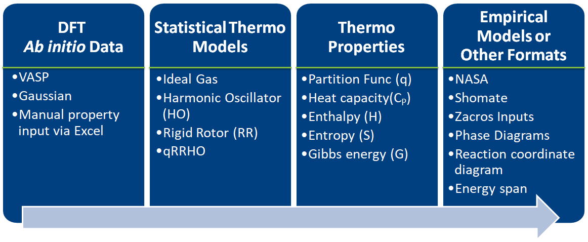
|-- 1.1. Some of pMuTT's Capabilities
| 2. Useful Links
| 3. Creating statistical mechanical objects using StatMech
|-- 3.1. Supported StatMech models
|--|-- 3.1.1. Translations
|--|-- 3.1.2. Vibrations
|--|-- 3.1.3. Rotations
|--|-- 3.1.4. Electronic
|--|-- 3.1.5. Miscellaneous
|-- 3.2. Initializing StatMech modes individually
|-- 3.3. Initializing StatMech modes using presets
| 4. Creating empirical objects
|-- 4.1. Inputting a NASA polynomial directly
|-- 4.2. Fitting an empirical object to a StatMech object
| 5. Input/Output
|-- 5.1. Input via Excel
| 6. Reactions
1. Introduction
![]()
- Estimates thermochemical and kinetic parameters using statistical mechanics, transition state theory
- Writes input files for kinetic models and eases thermodynamic analysis
- Implemented in Python
- Easy to learn
- Heavily used in scientific community
- Object-oriented approach is a natural analogy to chemical phenomenon
- Library approach allows users to define the starting point and end point
1.1 Some of pMuTT's Capabilities
Reaction Coordinate Diagrams
See the thermodynamic and kinetic feasibility of reaction mechanisms.

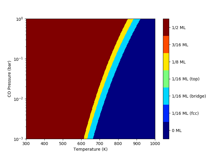
Ab-Initio Phase Diagrams
Predict the most stable configuration with respect to temperature and pressure.
Configurations
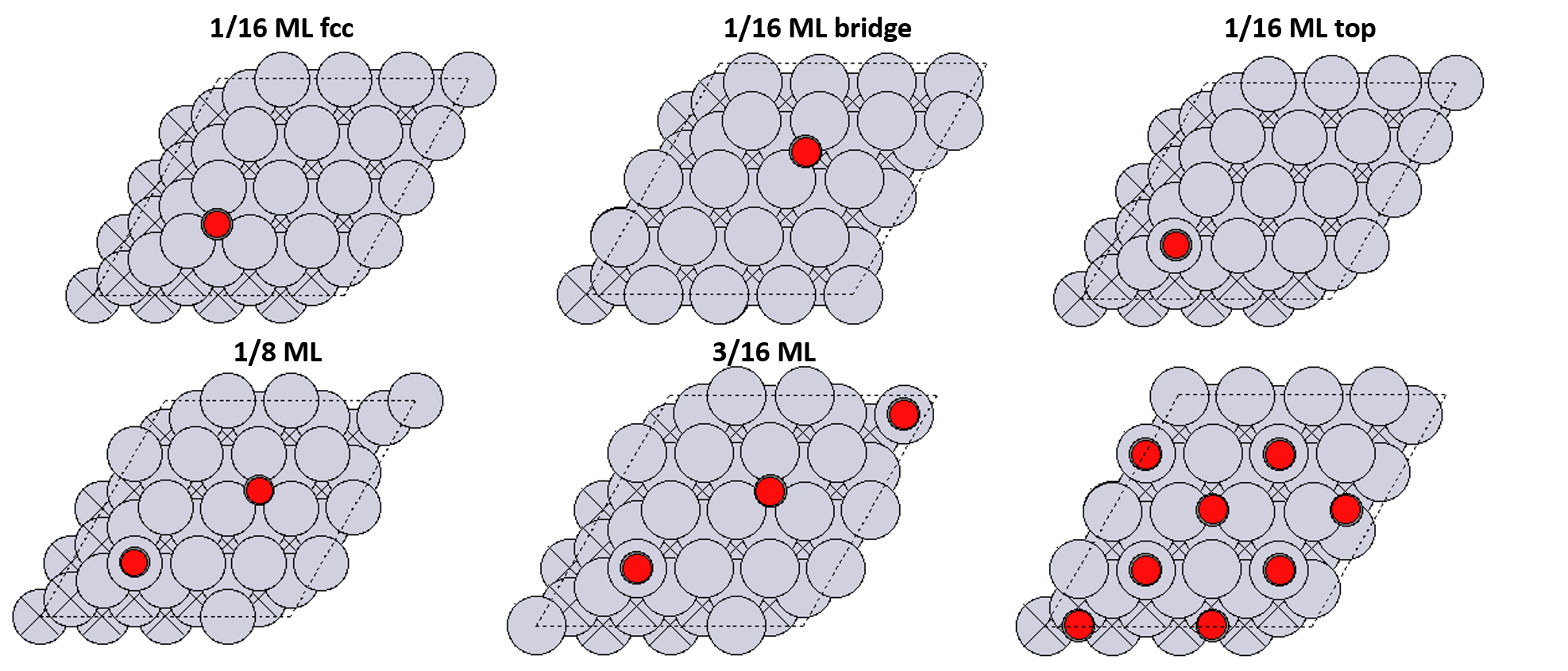 Typically we would consider more configurations than this.
1D Phase Diagram

2D Phase Diagram
2. Useful Links
- Documentation: find the most updated documentation
- Issues: report bugs, request features, receive help
- Examples: see examples
3. Creating statistical mechanical objects using StatMech
Molecules show translational, vibrational, rotational, electronic, and nuclear modes.
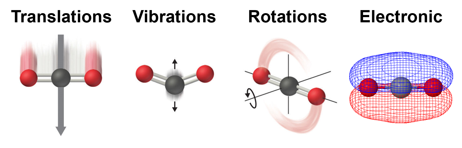
3.1. Supported StatMech modes
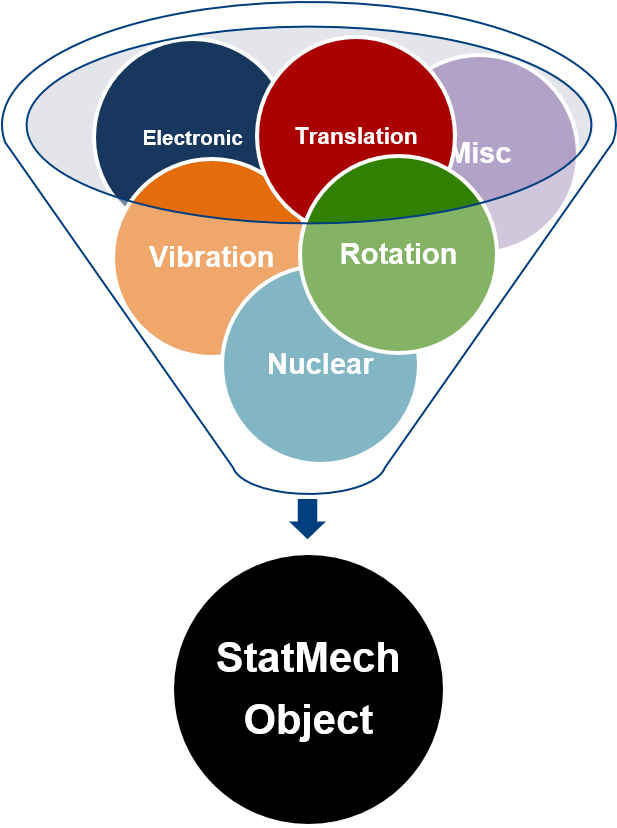
The StatMech object allows us to specify translational, vibrational, rotational, electronic and nuclear modes independently, which gives flexibility in what behavior you would like. Below are the available modes.
3.1.2. Vibrations
HarmonicVib- Harmonic vibrationsQRRHOVib- Quasi rigid rotor harmonic oscillator. Low frequency modes are treated as rigid rotations.EinsteinVib- Each atom in the crystal vibrates as independent 3D harmonic oscillatorsDebyeVib- Improves uponEinsteinVibby considering simultaneous vibrations. Improves accuracy at lower temperatures.
3.1.3. Rotations
RigidRotor- Molecule can be rotated with no change in bond properties
3.1.4. Electronic
GroundStateElec- Electronic ground state of the systemLSR- Linear Scaling Relationship to estimate binding energies using reference adsorbate
3.1.5. Miscellaneous
EmptyMode- Default mode if not specified. Does not contribute to any propertiesConstantMode- Specify arbitrary values to thermodynamic quantities
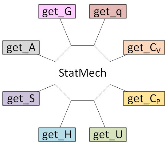
Using a StatMech mode gives you access to all the common thermodynamic properties.
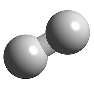
For this example, we will use a hydrogen molecule as an ideal gas:
- translations with no interaction between molecules
- harmonic vibrations
- rigid rotor rotations
- ground state electronic structure
- no contribution from nuclear modes.
3.2. Initializing StatMech modes individually
First, we will create an ASE Atoms object of H2. This will make it easier to initialize translations and rotations.
from ase.build import molecule
from ase.visualize import view

H2_atoms = molecule('H2')
view(H2_atoms)
Now we will initialize each mode separately
from pmutt.statmech import StatMech, trans, vib, rot, elec

'''Translational'''
H2_trans = trans.FreeTrans(n_degrees=3, atoms=H2_atoms)

'''Vibrational'''
H2_vib = vib.HarmonicVib(vib_wavenumbers=[4342.]) # vib_wavenumbers in cm-1

'''Rotational'''
H2_rot = rot.RigidRotor(symmetrynumber=2, atoms=H2_atoms)

'''Electronic'''
H2_elec = elec.GroundStateElec(potentialenergy=-6.77,spin=0) # potentialenergy in eV

'''StatMech Initialization'''
H2_statmech = StatMech(name='H2',
                       trans_model=H2_trans,
                       vib_model=H2_vib,
                       rot_model=H2_rot,
                       elec_model=H2_elec)

'''Calculate thermodynamic properties per mole basis'''
H_statmech = H2_statmech.get_H(T=298., units='kJ/mol')
S_statmech = H2_statmech.get_S(T=298., units='J/mol/K')
print('H_H2(T=298 K) = {:.1f} kJ/mol'.format(H_statmech))
print('S_H2(T=298 K) = {:.2f} J/mol/K'.format(S_statmech))
If you specify the composition of your species, you can calculate per mass quantities too.
'''Input composition'''
H2_statmech.elements = {'H': 2}

'''Calculate thermodynamic properties per mass basis'''
H_statmech = H2_statmech.get_H(T=298., units='kJ/g')
S_statmech = H2_statmech.get_S(T=298., units='J/g/K')
print('H_H2(T=298 K) = {:.1f} kJ/g'.format(H_statmech))
print('S_H2(T=298 K) = {:.2f} J/g/K'.format(S_statmech))
3.3. Initializing StatMech modes using presets
Commonly used models can be accessed via presets. The currently supported models are:
idealgas- Ideal gasesharmonic- Typical for surface specieselectronic- Only has electronic modesplaceholder- No contribution to any propertyconstant- Use arbitrary constants to thermodynamic properties
from ase.build import molecule
from pmutt.statmech import StatMech, presets

H2_statmech = StatMech(atoms=molecule('H2'),
                       vib_wavenumbers=[4342.], # cm-1
                       symmetrynumber=2,
                       potentialenergy=-6.77, # eV
                       spin=0.,
                       **presets['idealgas'])

'''Calculate thermodynamic properties'''
H_statmech = H2_statmech.get_H(T=298., units='kJ/mol')
S_statmech = H2_statmech.get_S(T=298., units='J/mol/K')
print('H_H2(T=298 K) = {:.1f} kJ/mol'.format(H_statmech))
print('S_H2(T=298 K) = {:.2f} J/mol/K'.format(S_statmech))
4. Creating empirical objects
Currently, pMuTT supports
They can be initialized in three ways:
- inputting the polynomials directly
- from another model (e.g.
StatMech,Shomate) using (from_model) - from heat capacity, enthalpy and entropy data using (
from_data)
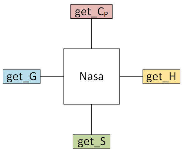
4.1. Inputting a NASA polynomial directly
The H2 NASA polynomial from the Burcat database is represented as:
H2                TPIS78H   2               G   200.000  3500.000  1000.000    1
 3.33727920E+00-4.94024731E-05 4.99456778E-07-1.79566394E-10 2.00255376E-14    2
-9.50158922E+02-3.20502331E+00 2.34433112E+00 7.98052075E-03-1.94781510E-05    3
 2.01572094E-08-7.37611761E-12-9.17935173E+02 6.83010238E-01                   4
This can be translated to pMuTT syntax using:
import numpy as np
from matplotlib import pyplot as plt

from pmutt import plot_1D
from pmutt.empirical.nasa import Nasa

# Initialize NASA polynomial
H2_nasa = Nasa(name='H2',
               elements={'H': 2},
               phase='G',
               T_low=200., T_mid=1000., T_high=3500.,
               a_low=[2.34433112E+00, 7.98052075E-03, -1.94781510E-05,
                      2.01572094E-08, -7.37611761E-12, -9.17935173E+02,
                      6.83010238E-01],
               a_high=[3.33727920E+00, -4.94024731E-05, 4.99456778E-07,
                       -1.79566394E-10, 2.00255376E-14, -9.50158922E+02,
                       -3.20502331E+00])

# Calculate thermodynamic quantities using the same syntax as StatMech
H_H2 = H2_nasa.get_H(units='kcal/mol', T=298.)
print('H_H2(T=298 K) = {} kcal/mol'.format(H_H2))

# Show thermodynamic quantities vs. T
T = np.linspace(200., 3500.)
f2, ax2 = plot_1D(H2_nasa,
                  x_name='T', x_values=T,
                  methods=('get_H', 'get_S', 'get_G'),
                  get_H_kwargs={'units': 'kcal/mol'},
                  get_S_kwargs={'units': 'cal/mol/K'},
                  get_G_kwargs={'units': 'kcal/mol'})

# Modifying figure
ax2[0].set_ylabel('H (kcal/mol)')
ax2[1].set_ylabel('S (cal/mol/K)')
ax2[2].set_ylabel('G (kcal/mol)')
ax2[2].set_xlabel('T (K)')
f2.set_size_inches(5, 5)
f2.set_dpi(200)
plt.show()

4.2. Fitting an empirical object to a StatMech object
Empirical objects can be made directly any species objects using the from_model method.
H2_nasa = Nasa.from_model(name='H2',
                          T_low=200.,
                          T_high=3500.,
                          model=H2_statmech)
# Compare the statistical mechanical model to the empirical model
f3, ax3 = H2_nasa.plot_statmech_and_empirical(Cp_units='J/mol/K',
                                              H_units='kJ/mol',
                                              S_units='J/mol/K',
                                              G_units='kJ/mol')
f3.set_size_inches(6, 8)
f3.set_dpi(150)
plt.show()

from pmutt.empirical.shomate import Shomate

H2_shomate = Shomate.from_model(model=H2_nasa)

# Compare the statistical mechanical model to the empirical model
f3, ax3 = H2_shomate.plot_statmech_and_empirical(Cp_units='J/mol/K',
                                                 H_units='kJ/mol',
                                                 S_units='J/mol/K',
                                                 G_units='kJ/mol')
f3.set_size_inches(6, 8)
f3.set_dpi(150)
plt.show()

The Shomate is a simpler polynomial than the Nasa polynomial so it does not capture the features as well for the large T range. It is always a good idea to check your fit.
5. Input/Output
pMuTT has more IO functionality than below. See this page for supported IO functions.
5.1. Input via Excel
Encoding each object in Python can be tedious. You can read several species from Excel spreadsheets using pmutt.io.excel.read_excel. Note that this function returns a list of dictionaries. This output allows you to initialize whichever object you want using kwargs syntax. There are also special rules that depend on the header name.
Below, we show an example importing species data from a spreadsheet and creating a series of NASA polynomials.
First, we ensure that the current working directory is the same as the notebook so we can access the spreadsheet.
import os
from pathlib import Path

# Find the location of Jupyter notebook
# Note that normally Python scripts have a __file__ variable but Jupyter notebook doesn't.
# Using pathlib can overcome this limiation
try:
    notebook_path = os.path.dirname(__file__)
except NameError:
    notebook_path = Path().resolve()
os.chdir(notebook_path)
Now we can read from the spreadsheet.
from pprint import pprint
from pmutt.io.excel import read_excel

ab_initio_data = read_excel(io='./input/NH3_Input_Data.xlsx', sheet_name='species')
pprint(ab_initio_data)
After the data is read, we can fit the Nasa objects from the statistical mechanical data.
from pmutt.empirical.nasa import Nasa

# Create NASA polynomials using **kwargs syntax
nasa_species = []
for species_data in ab_initio_data:
    single_nasa_species = Nasa.from_model(T_low=100.,
                                          T_high=1500.,
                                          **species_data)
    nasa_species.append(single_nasa_species)
Just to ensure the species were read correctly, we can try printing out thermodynamic values.
import pandas as pd

thermo_data = {'Name': [],
               'H (kcal/mol)': [],
               'S (cal/mol/K)': [],
               'G (kcal/mol)': []}

'''Calculate properties at 298 K'''
T = 298. # K
for single_nasa_species in nasa_species:
    thermo_data['Name'].append(single_nasa_species.name)
    thermo_data['H (kcal/mol)'].append(single_nasa_species.get_H(units='kcal/mol', T=T))
    thermo_data['S (cal/mol/K)'].append(single_nasa_species.get_S(units='cal/mol/K', T=T))
    thermo_data['G (kcal/mol)'].append(single_nasa_species.get_G(units='kcal/mol', T=T))

'''Create Pandas Dataframe for easy printing'''
columns = ['Name', 'H (kcal/mol)', 'S (cal/mol/K)', 'G (kcal/mol)']
thermo_data = pd.DataFrame(thermo_data, columns=columns)
print(thermo_data)
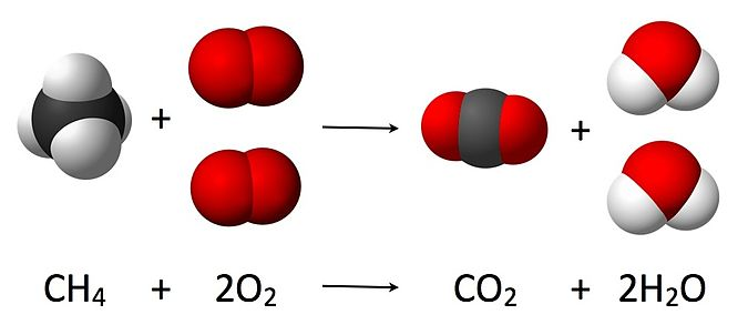
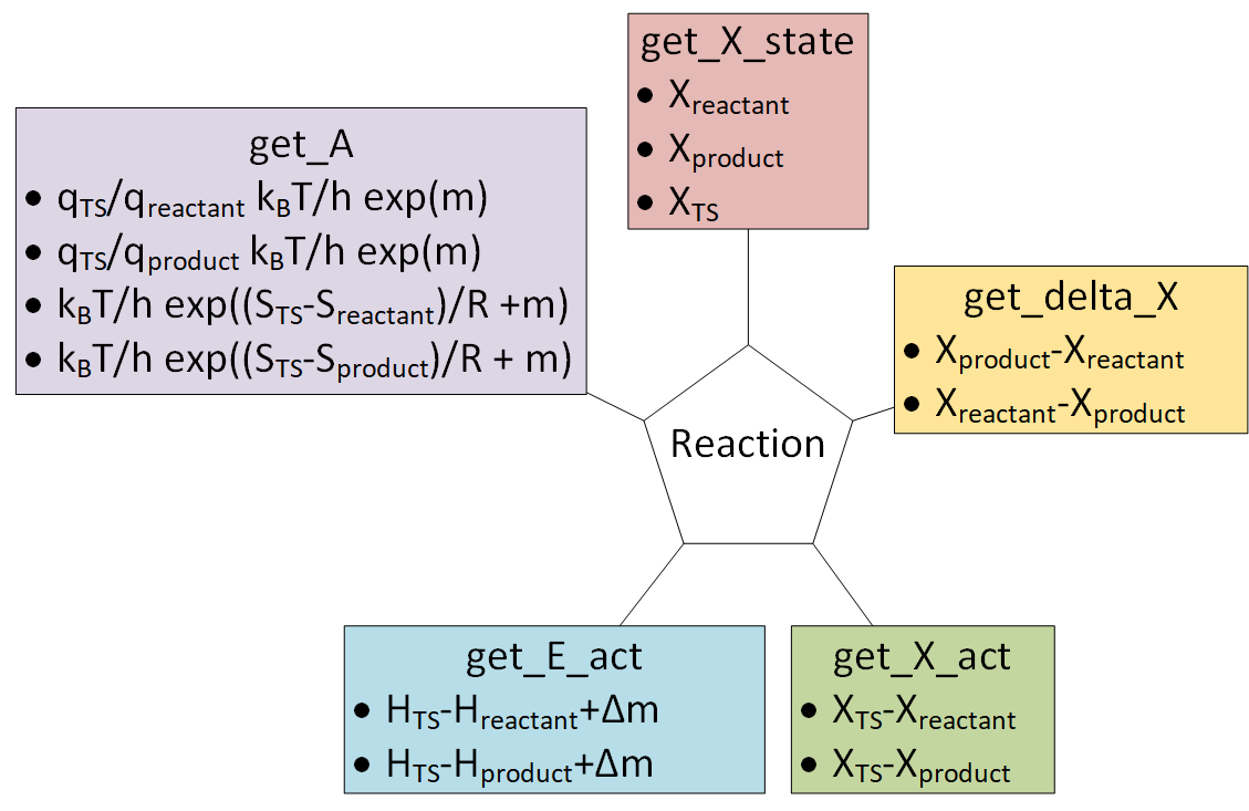
6. Reactions
Reaction objects can be created by putting together Nasa, Nasa9, Shomate and StatMech objects.

6.1. Initializing Reaction objects using from_string
The from_string method is the easiest way to create a Reaction object. It requires the relevant species to be in a dictionary and a string to describe the reaction.

We will demonstrate its use for the formation of NH3.
from pmutt.empirical.nasa import Nasa
from pmutt.empirical.shomate import Shomate
from pmutt.reaction import Reaction

# Create species. Note that you can mix different types of species
species = {
    'H2': StatMech(name='H2', atoms=molecule('H2'),
                   vib_wavenumbers=[4342.], # cm-1
                   symmetrynumber=2,
                   potentialenergy=-6.77, # eV
                   spin=0.,
                   **presets['idealgas']),
    'N2': Nasa(name='N2', T_low=300., T_mid=643., T_high=1000.,
               a_low=[3.3956319945669633, 0.001115707689025668,
                      -4.301993779374381e-06, 6.8071424019295535e-09,
                      -3.2903312791047058e-12, -191001.55648623788,
                      3.556111439828502],
               a_high=[4.050329990684662, -0.0029677854067980108,
                       5.323485005316287e-06, -3.3518122405333548e-09,
                       7.58446718337381e-13, -191086.2004520406,
                       0.6858235504924011]),
    'NH3': Shomate(name='NH3', T_low=300., T_high=1000.,
                   a=[18.792357134351683, 44.82725349479501,
                      -10.05898449447048, 0.3711633831565547,
                      0.2969942466370908, -1791.225746924463,
                      203.9035662274934, 1784.714638346206]),
}

# Define the formation of ammonia reaction
rxn = Reaction.from_string('1.5H2 + 0.5N2 = NH3', species)
Now we can calculate thermodynamic properties of the reaction.
'''Forward change in enthalpy'''
H_rxn_fwd = rxn.get_delta_H(units='kcal/mol', T=300.)
print('Delta H_fwd(T = 300 K) = {:.1f} kcal/mol'.format(H_rxn_fwd))

'''Reverse change in entropy'''
S_rxn_rev = rxn.get_delta_S(units='cal/mol/K', T=300., rev=True)
print('Delta S_rev(T = 300 K) = {:.1f} cal/mol/K'.format(S_rxn_rev))

'''Gibbs energy of reactants'''
G_react = rxn.get_G_state(units='kcal/mol', T=300., state='reactants')
print('G_reactants(T = 300 K) = {:.1f} kcal/mol'.format(G_react))