#!/usr/bin/env python
# coding: utf-8
# # AIChE 2019 pMuTT Workshop
#
# Instructions and materials for the Computational Catalysis workshop can be found on webpage.
#
# # Table of Contents
#
# | **1\. [Introduction](#section_1)**
#
# |-- **1.1. [Some of pMuTT's Capabilities](#section_1_1)**
#
# | **2\. [Useful Links](#section_2)**
#
# | **3\. [Creating statistical mechanical objects using StatMech](#section_3)**
#
# |-- **3.1. [Supported StatMech models](#section_3_1)**
#
# |--|-- **3.1.1. [Translations](#section_3_1_1)**
#
# |--|-- **3.1.2. [Vibrations](#section_3_1_2)**
#
# |--|-- **3.1.3. [Rotations](#section_3_1_3)**
#
# |--|-- **3.1.4. [Electronic](#section_3_1_4)**
#
# |--|-- **3.1.5. [Miscellaneous](#section_3_1_5)**
#
# |-- **3.2. [Initializing StatMech modes individually](#section_3_2)**
#
# |-- **3.3. [Initializing StatMech modes using presets](#section_3_3)**
#
# | **4\. [Creating empirical objects](#section_4)**
#
# |-- **4.1. [Inputting a NASA polynomial directly](#section_4_1)**
#
# |-- **4.2. [Fitting an empirical object to a StatMech object](#section_4_2)**
#
# | **5\. [Input/Output](#section_5)**
#
# |-- **5.1. [Input via Excel](#section_5_1)**
#
# | **6\. [Reactions](#section_6)**
#
# |-- **6.1. [Initializing Reaction objects using from_string](#section_6_1)**
#
# # 1. Introduction
#
#  #
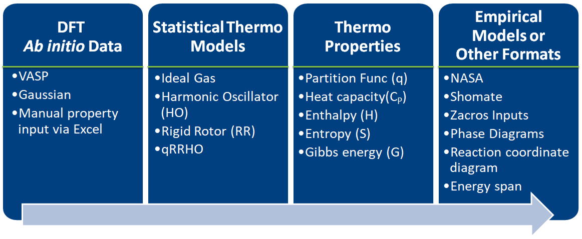
# - Estimates thermochemical and kinetic parameters using statistical mechanics, transition state theory
# - Writes input files for kinetic models and eases thermodynamic analysis
# - Implemented in Python
# - Easy to learn
# - Heavily used in scientific community
# - Object-oriented approach is a natural analogy to chemical phenomenon
# - Library approach allows users to define the starting point and end point
#
#
#
# - Estimates thermochemical and kinetic parameters using statistical mechanics, transition state theory
# - Writes input files for kinetic models and eases thermodynamic analysis
# - Implemented in Python
# - Easy to learn
# - Heavily used in scientific community
# - Object-oriented approach is a natural analogy to chemical phenomenon
# - Library approach allows users to define the starting point and end point
#
#  #
# ## 1.1 Some of pMuTT's Capabilities
# ### Reaction Coordinate Diagrams
#
# See the thermodynamic and kinetic feasibility of reaction mechanisms.
#
#
#
# ## 1.1 Some of pMuTT's Capabilities
# ### Reaction Coordinate Diagrams
#
# See the thermodynamic and kinetic feasibility of reaction mechanisms.
#
#  #
# ### Ab-Initio Phase Diagrams
#
# Predict the most stable configuration with respect to temperature and pressure.
#
# **Configurations**
#
#
# ### Ab-Initio Phase Diagrams
#
# Predict the most stable configuration with respect to temperature and pressure.
#
# **Configurations**
# 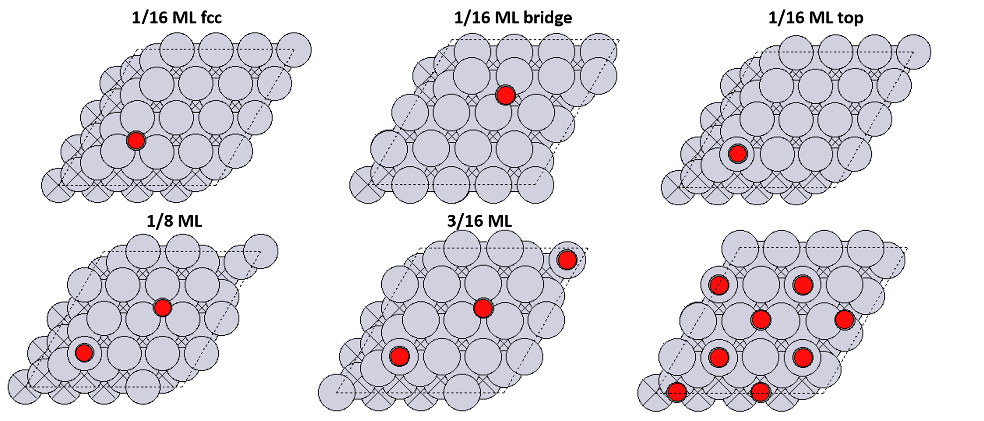 # Typically we would consider more configurations than this.
#
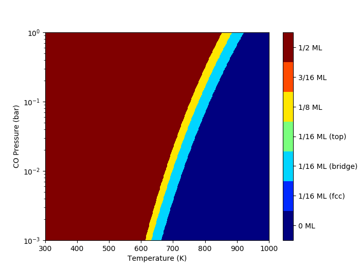
# **1D Phase Diagram**
#
# Typically we would consider more configurations than this.
#
# **1D Phase Diagram**
#  #
# **2D Phase Diagram**
#
#
# **2D Phase Diagram**
#  #
# # 2. Useful Links
#
# - [Documentation](https://vlachosgroup.github.io/pMuTT/): find the most updated documentation
# - [Issues](https://github.com/VlachosGroup/pmutt/issues): report bugs, request features, receive help
# - [Examples](https://vlachosgroup.github.io/pMuTT/examples.html): see examples
#
# # 3. Creating statistical mechanical objects using StatMech
#
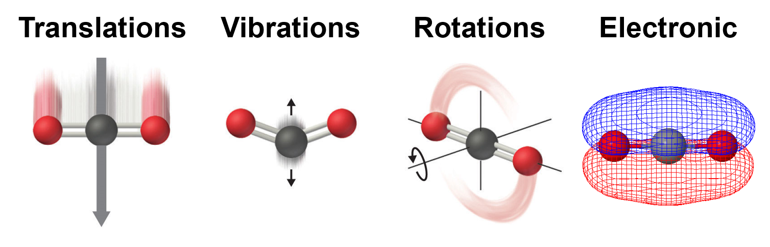
# Molecules show translational, vibrational, rotational, electronic, and nuclear modes.
#
#
#
# # 2. Useful Links
#
# - [Documentation](https://vlachosgroup.github.io/pMuTT/): find the most updated documentation
# - [Issues](https://github.com/VlachosGroup/pmutt/issues): report bugs, request features, receive help
# - [Examples](https://vlachosgroup.github.io/pMuTT/examples.html): see examples
#
# # 3. Creating statistical mechanical objects using StatMech
#
# Molecules show translational, vibrational, rotational, electronic, and nuclear modes.
#
#  #
# ## 3.1. Supported StatMech modes
#
#
#
# ## 3.1. Supported StatMech modes
#
# 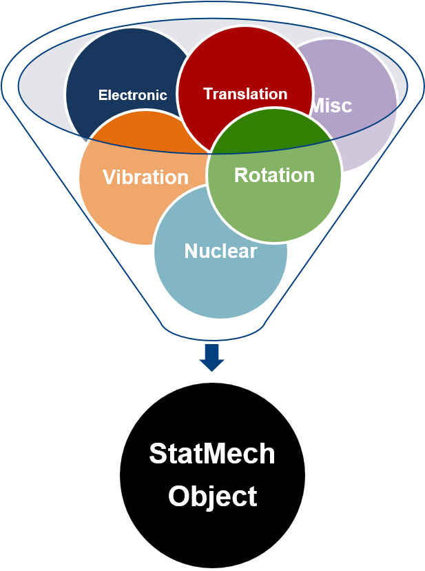 #
# The StatMech object allows us to specify translational, vibrational, rotational, electronic and nuclear modes independently, which gives flexibility in what behavior you would like. Below are the available modes.
#
# ### 3.1.1. Translations
# - [``FreeTrans``](https://vlachosgroup.github.io/pMuTT/statmech.html#freetrans) - Translations assuming no intermolecular interactions. Can be adjusted for 1, 2, or 3 degrees of translation.
#
# ### 3.1.2. Vibrations
# - [``HarmonicVib``](https://vlachosgroup.github.io/pMuTT/statmech.html#harmonicvib) - Harmonic vibrations
# - [``QRRHOVib``](https://vlachosgroup.github.io/pMuTT/statmech.html#harmonicvib) - Quasi rigid rotor harmonic oscillator. Low frequency modes are treated as rigid rotations.
# - [``EinsteinVib``](https://vlachosgroup.github.io/pMuTT/statmech.html#einsteinvib) - Each atom in the crystal vibrates as independent 3D harmonic oscillators
# - [``DebyeVib``](https://vlachosgroup.github.io/pMuTT/statmech.html#debyevib) - Improves upon ``EinsteinVib`` by considering simultaneous vibrations. Improves accuracy at lower temperatures.
#
# ### 3.1.3. Rotations
# - [``RigidRotor``](https://vlachosgroup.github.io/pMuTT/statmech.html#rigidrotor) - Molecule can be rotated with no change in bond properties
#
# ### 3.1.4. Electronic
# - [``GroundStateElec``](https://vlachosgroup.github.io/pMuTT/statmech.html#groundstateelec) - Electronic ground state of the system
# - [``LSR``](https://vlachosgroup.github.io/pMuTT/statmech.html#linear-scaling-relationships-lsrs) - Linear Scaling Relationship to estimate binding energies using reference adsorbate
#
# ### 3.1.5. Miscellaneous
# - [``EmptyMode``](https://vlachosgroup.github.io/pMuTT/statmech.html#empty-mode) - Default mode if not specified. Does not contribute to any properties
# - [``ConstantMode``](https://vlachosgroup.github.io/pMuTT/statmech.html#constant-mode) - Specify arbitrary values to thermodynamic quantities
#
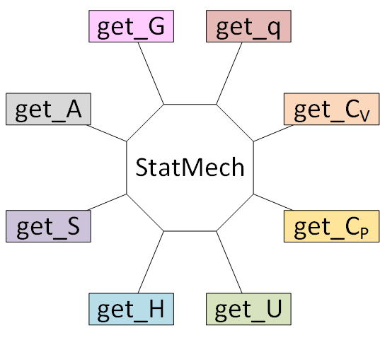
# Using a ``StatMech`` mode gives you access to all the common thermodynamic properties.
#
#
#
# The StatMech object allows us to specify translational, vibrational, rotational, electronic and nuclear modes independently, which gives flexibility in what behavior you would like. Below are the available modes.
#
# ### 3.1.1. Translations
# - [``FreeTrans``](https://vlachosgroup.github.io/pMuTT/statmech.html#freetrans) - Translations assuming no intermolecular interactions. Can be adjusted for 1, 2, or 3 degrees of translation.
#
# ### 3.1.2. Vibrations
# - [``HarmonicVib``](https://vlachosgroup.github.io/pMuTT/statmech.html#harmonicvib) - Harmonic vibrations
# - [``QRRHOVib``](https://vlachosgroup.github.io/pMuTT/statmech.html#harmonicvib) - Quasi rigid rotor harmonic oscillator. Low frequency modes are treated as rigid rotations.
# - [``EinsteinVib``](https://vlachosgroup.github.io/pMuTT/statmech.html#einsteinvib) - Each atom in the crystal vibrates as independent 3D harmonic oscillators
# - [``DebyeVib``](https://vlachosgroup.github.io/pMuTT/statmech.html#debyevib) - Improves upon ``EinsteinVib`` by considering simultaneous vibrations. Improves accuracy at lower temperatures.
#
# ### 3.1.3. Rotations
# - [``RigidRotor``](https://vlachosgroup.github.io/pMuTT/statmech.html#rigidrotor) - Molecule can be rotated with no change in bond properties
#
# ### 3.1.4. Electronic
# - [``GroundStateElec``](https://vlachosgroup.github.io/pMuTT/statmech.html#groundstateelec) - Electronic ground state of the system
# - [``LSR``](https://vlachosgroup.github.io/pMuTT/statmech.html#linear-scaling-relationships-lsrs) - Linear Scaling Relationship to estimate binding energies using reference adsorbate
#
# ### 3.1.5. Miscellaneous
# - [``EmptyMode``](https://vlachosgroup.github.io/pMuTT/statmech.html#empty-mode) - Default mode if not specified. Does not contribute to any properties
# - [``ConstantMode``](https://vlachosgroup.github.io/pMuTT/statmech.html#constant-mode) - Specify arbitrary values to thermodynamic quantities
#
# Using a ``StatMech`` mode gives you access to all the common thermodynamic properties.
#
#  #
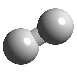
# For this example, we will use a hydrogen molecule as an ideal gas:
# - translations with no interaction between molecules
# - harmonic vibrations
# - rigid rotor rotations
# - ground state electronic structure
# - no contribution from nuclear modes.
#
#
#
# For this example, we will use a hydrogen molecule as an ideal gas:
# - translations with no interaction between molecules
# - harmonic vibrations
# - rigid rotor rotations
# - ground state electronic structure
# - no contribution from nuclear modes.
#
#  #
# ## 3.2. Initializing StatMech modes individually
# First, we will create an ASE Atoms object of H2. This will make it easier to initialize translations and rotations.
# In[1]:
from ase.build import molecule
from ase.visualize import view
H2_atoms = molecule('H2')
view(H2_atoms)
# Now we will initialize each mode separately
# In[2]:
from pmutt.statmech import StatMech, trans, vib, rot, elec
'''Translational'''
H2_trans = trans.FreeTrans(n_degrees=3, atoms=H2_atoms)
'''Vibrational'''
H2_vib = vib.HarmonicVib(vib_wavenumbers=[4342.]) # vib_wavenumbers in cm-1
'''Rotational'''
H2_rot = rot.RigidRotor(symmetrynumber=2, atoms=H2_atoms)
'''Electronic'''
H2_elec = elec.GroundStateElec(potentialenergy=-6.77,spin=0) # potentialenergy in eV
'''StatMech Initialization'''
H2_statmech = StatMech(name='H2',
trans_model=H2_trans,
vib_model=H2_vib,
rot_model=H2_rot,
elec_model=H2_elec)
'''Calculate thermodynamic properties per mole basis'''
H_statmech = H2_statmech.get_H(T=298., units='kJ/mol')
S_statmech = H2_statmech.get_S(T=298., units='J/mol/K')
print('H_H2(T=298 K) = {:.1f} kJ/mol'.format(H_statmech))
print('S_H2(T=298 K) = {:.2f} J/mol/K'.format(S_statmech))
# If you specify the composition of your species, you can calculate per mass quantities too.
# In[3]:
'''Input composition'''
H2_statmech.elements = {'H': 2}
'''Calculate thermodynamic properties per mass basis'''
H_statmech = H2_statmech.get_H(T=298., units='kJ/g')
S_statmech = H2_statmech.get_S(T=298., units='J/g/K')
print('H_H2(T=298 K) = {:.1f} kJ/g'.format(H_statmech))
print('S_H2(T=298 K) = {:.2f} J/g/K'.format(S_statmech))
#
# ## 3.3. Initializing StatMech modes using presets
#
# Commonly used models can be accessed via [``presets``](https://vlachosgroup.github.io/pMuTT/statmech.html#presets). The currently supported models are:
#
# - [``idealgas``](https://vlachosgroup.github.io/pMuTT/statmech.html#ideal-gas-idealgas) - Ideal gases
# - [``harmonic``](https://vlachosgroup.github.io/pMuTT/statmech.html#harmonic-approximation-harmonic) - Typical for surface species
# - [``electronic``](https://vlachosgroup.github.io/pMuTT/statmech.html#electronic-electronic) - Only has electronic modes
# - [``placeholder``](https://vlachosgroup.github.io/pMuTT/statmech.html#placeholder-placeholder) - No contribution to any property
# - [``constant``](https://vlachosgroup.github.io/pMuTT/statmech.html#constant-constant) - Use arbitrary constants to thermodynamic properties
#
# In[4]:
from ase.build import molecule
from pmutt.statmech import StatMech, presets
H2_statmech = StatMech(atoms=molecule('H2'),
vib_wavenumbers=[4342.], # cm-1
symmetrynumber=2,
potentialenergy=-6.77, # eV
spin=0.,
**presets['idealgas'])
'''Calculate thermodynamic properties'''
H_statmech = H2_statmech.get_H(T=298., units='kJ/mol')
S_statmech = H2_statmech.get_S(T=298., units='J/mol/K')
print('H_H2(T=298 K) = {:.1f} kJ/mol'.format(H_statmech))
print('S_H2(T=298 K) = {:.2f} J/mol/K'.format(S_statmech))
#
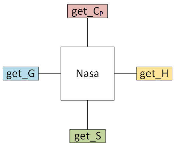
# # 4. Creating empirical objects
# Currently, pMuTT supports
#
# - [NASA polynomials](https://vlachosgroup.github.io/pMuTT/empirical.html#nasa)
# - [NASA9 polynomials](https://vlachosgroup.github.io/pMuTT/empirical.html#nasa9)
# - [Shomate polynomials](https://vlachosgroup.github.io/pMuTT/empirical.html#shomate).
#
# They can be initialized in three ways:
# - inputting the polynomials directly
# - from another model (e.g. ``StatMech``, ``Shomate``) using (``from_model``)
# - from heat capacity, enthalpy and entropy data using (``from_data``)
#
#
#
# ## 3.2. Initializing StatMech modes individually
# First, we will create an ASE Atoms object of H2. This will make it easier to initialize translations and rotations.
# In[1]:
from ase.build import molecule
from ase.visualize import view
H2_atoms = molecule('H2')
view(H2_atoms)
# Now we will initialize each mode separately
# In[2]:
from pmutt.statmech import StatMech, trans, vib, rot, elec
'''Translational'''
H2_trans = trans.FreeTrans(n_degrees=3, atoms=H2_atoms)
'''Vibrational'''
H2_vib = vib.HarmonicVib(vib_wavenumbers=[4342.]) # vib_wavenumbers in cm-1
'''Rotational'''
H2_rot = rot.RigidRotor(symmetrynumber=2, atoms=H2_atoms)
'''Electronic'''
H2_elec = elec.GroundStateElec(potentialenergy=-6.77,spin=0) # potentialenergy in eV
'''StatMech Initialization'''
H2_statmech = StatMech(name='H2',
trans_model=H2_trans,
vib_model=H2_vib,
rot_model=H2_rot,
elec_model=H2_elec)
'''Calculate thermodynamic properties per mole basis'''
H_statmech = H2_statmech.get_H(T=298., units='kJ/mol')
S_statmech = H2_statmech.get_S(T=298., units='J/mol/K')
print('H_H2(T=298 K) = {:.1f} kJ/mol'.format(H_statmech))
print('S_H2(T=298 K) = {:.2f} J/mol/K'.format(S_statmech))
# If you specify the composition of your species, you can calculate per mass quantities too.
# In[3]:
'''Input composition'''
H2_statmech.elements = {'H': 2}
'''Calculate thermodynamic properties per mass basis'''
H_statmech = H2_statmech.get_H(T=298., units='kJ/g')
S_statmech = H2_statmech.get_S(T=298., units='J/g/K')
print('H_H2(T=298 K) = {:.1f} kJ/g'.format(H_statmech))
print('S_H2(T=298 K) = {:.2f} J/g/K'.format(S_statmech))
#
# ## 3.3. Initializing StatMech modes using presets
#
# Commonly used models can be accessed via [``presets``](https://vlachosgroup.github.io/pMuTT/statmech.html#presets). The currently supported models are:
#
# - [``idealgas``](https://vlachosgroup.github.io/pMuTT/statmech.html#ideal-gas-idealgas) - Ideal gases
# - [``harmonic``](https://vlachosgroup.github.io/pMuTT/statmech.html#harmonic-approximation-harmonic) - Typical for surface species
# - [``electronic``](https://vlachosgroup.github.io/pMuTT/statmech.html#electronic-electronic) - Only has electronic modes
# - [``placeholder``](https://vlachosgroup.github.io/pMuTT/statmech.html#placeholder-placeholder) - No contribution to any property
# - [``constant``](https://vlachosgroup.github.io/pMuTT/statmech.html#constant-constant) - Use arbitrary constants to thermodynamic properties
#
# In[4]:
from ase.build import molecule
from pmutt.statmech import StatMech, presets
H2_statmech = StatMech(atoms=molecule('H2'),
vib_wavenumbers=[4342.], # cm-1
symmetrynumber=2,
potentialenergy=-6.77, # eV
spin=0.,
**presets['idealgas'])
'''Calculate thermodynamic properties'''
H_statmech = H2_statmech.get_H(T=298., units='kJ/mol')
S_statmech = H2_statmech.get_S(T=298., units='J/mol/K')
print('H_H2(T=298 K) = {:.1f} kJ/mol'.format(H_statmech))
print('S_H2(T=298 K) = {:.2f} J/mol/K'.format(S_statmech))
#
# # 4. Creating empirical objects
# Currently, pMuTT supports
#
# - [NASA polynomials](https://vlachosgroup.github.io/pMuTT/empirical.html#nasa)
# - [NASA9 polynomials](https://vlachosgroup.github.io/pMuTT/empirical.html#nasa9)
# - [Shomate polynomials](https://vlachosgroup.github.io/pMuTT/empirical.html#shomate).
#
# They can be initialized in three ways:
# - inputting the polynomials directly
# - from another model (e.g. ``StatMech``, ``Shomate``) using (``from_model``)
# - from heat capacity, enthalpy and entropy data using (``from_data``)
#
#  #
# ## 4.1. Inputting a NASA polynomial directly
#
# The H2 NASA polynomial from the [Burcat database](http://combustion.berkeley.edu/gri_mech/version30/files30/thermo30.dat) is represented as:
#
# ```
# H2 TPIS78H 2 G 200.000 3500.000 1000.000 1
# 3.33727920E+00-4.94024731E-05 4.99456778E-07-1.79566394E-10 2.00255376E-14 2
# -9.50158922E+02-3.20502331E+00 2.34433112E+00 7.98052075E-03-1.94781510E-05 3
# 2.01572094E-08-7.37611761E-12-9.17935173E+02 6.83010238E-01 4
# ```
#
# This can be translated to pMuTT syntax using:
# In[5]:
import numpy as np
from matplotlib import pyplot as plt
from pmutt import plot_1D
from pmutt.empirical.nasa import Nasa
# Initialize NASA polynomial
H2_nasa = Nasa(name='H2',
elements={'H': 2},
phase='G',
T_low=200., T_mid=1000., T_high=3500.,
a_low=[2.34433112E+00, 7.98052075E-03, -1.94781510E-05,
2.01572094E-08, -7.37611761E-12, -9.17935173E+02,
6.83010238E-01],
a_high=[3.33727920E+00, -4.94024731E-05, 4.99456778E-07,
-1.79566394E-10, 2.00255376E-14, -9.50158922E+02,
-3.20502331E+00])
# Calculate thermodynamic quantities using the same syntax as StatMech
H_H2 = H2_nasa.get_H(units='kcal/mol', T=298.)
print('H_H2(T=298 K) = {} kcal/mol'.format(H_H2))
# Show thermodynamic quantities vs. T
T = np.linspace(200., 3500.)
f2, ax2 = plot_1D(H2_nasa,
x_name='T', x_values=T,
methods=('get_H', 'get_S', 'get_G'),
get_H_kwargs={'units': 'kcal/mol'},
get_S_kwargs={'units': 'cal/mol/K'},
get_G_kwargs={'units': 'kcal/mol'})
# Modifying figure
ax2[0].set_ylabel('H (kcal/mol)')
ax2[1].set_ylabel('S (cal/mol/K)')
ax2[2].set_ylabel('G (kcal/mol)')
ax2[2].set_xlabel('T (K)')
f2.set_size_inches(5, 5)
f2.set_dpi(200)
plt.show()
#
# ## 4.2. Fitting an empirical object to a StatMech object
# Empirical objects can be made directly any species objects using the ``from_model`` method.
# In[6]:
H2_nasa = Nasa.from_model(name='H2',
T_low=200.,
T_high=3500.,
model=H2_statmech)
# Compare the statistical mechanical model to the empirical model
f3, ax3 = H2_nasa.plot_statmech_and_empirical(Cp_units='J/mol/K',
H_units='kJ/mol',
S_units='J/mol/K',
G_units='kJ/mol')
f3.set_size_inches(6, 8)
f3.set_dpi(150)
plt.show()
# In[7]:
from pmutt.empirical.shomate import Shomate
H2_shomate = Shomate.from_model(model=H2_nasa)
# Compare the statistical mechanical model to the empirical model
f3, ax3 = H2_shomate.plot_statmech_and_empirical(Cp_units='J/mol/K',
H_units='kJ/mol',
S_units='J/mol/K',
G_units='kJ/mol')
f3.set_size_inches(6, 8)
f3.set_dpi(150)
plt.show()
# The ``Shomate`` is a simpler polynomial than the ``Nasa`` polynomial so it does not capture the features as well for the large T range. It is always a good idea to check your fit.
#
# # 5. Input/Output
# pMuTT has more IO functionality than below. See this page for [supported IO functions](https://vlachosgroup.github.io/pMuTT/io.html).
#
# ## 5.1. Input via Excel
#
# Encoding each object in Python can be tedious. You can read several species from Excel spreadsheets using [``pmutt.io.excel.read_excel``](https://vlachosgroup.github.io/pmutt/io.html?highlight=read_excel#pmutt.io.excel.read_excel). Note that this function returns a list of dictionaries. This output allows you to initialize whichever object you want using kwargs syntax. There are also [special rules that depend on the header name](https://vlachosgroup.github.io/pMuTT/io.html#special-rules).
#
# Below, we show an example importing species data from a spreadsheet and creating a series of NASA polynomials.
# First, we ensure that the current working directory is the same as the notebook so we can access the spreadsheet.
# In[8]:
import os
from pathlib import Path
# Find the location of Jupyter notebook
# Note that normally Python scripts have a __file__ variable but Jupyter notebook doesn't.
# Using pathlib can overcome this limiation
try:
notebook_path = os.path.dirname(__file__)
except NameError:
notebook_path = Path().resolve()
os.chdir(notebook_path)
# Now we can read from the spreadsheet.
# In[9]:
from pprint import pprint
from pmutt.io.excel import read_excel
ab_initio_data = read_excel(io='./input/NH3_Input_Data.xlsx', sheet_name='species')
pprint(ab_initio_data)
# After the data is read, we can fit the ``Nasa`` objects from the statistical mechanical data.
# In[10]:
from pmutt.empirical.nasa import Nasa
# Create NASA polynomials using **kwargs syntax
nasa_species = []
for species_data in ab_initio_data:
single_nasa_species = Nasa.from_model(T_low=100.,
T_high=1500.,
**species_data)
nasa_species.append(single_nasa_species)
# Just to ensure the species were read correctly, we can try printing out thermodynamic values.
# In[11]:
import pandas as pd
thermo_data = {'Name': [],
'H (kcal/mol)': [],
'S (cal/mol/K)': [],
'G (kcal/mol)': []}
'''Calculate properties at 298 K'''
T = 298. # K
for single_nasa_species in nasa_species:
thermo_data['Name'].append(single_nasa_species.name)
thermo_data['H (kcal/mol)'].append(single_nasa_species.get_H(units='kcal/mol', T=T))
thermo_data['S (cal/mol/K)'].append(single_nasa_species.get_S(units='cal/mol/K', T=T))
thermo_data['G (kcal/mol)'].append(single_nasa_species.get_G(units='kcal/mol', T=T))
'''Create Pandas Dataframe for easy printing'''
columns = ['Name', 'H (kcal/mol)', 'S (cal/mol/K)', 'G (kcal/mol)']
thermo_data = pd.DataFrame(thermo_data, columns=columns)
print(thermo_data)
#
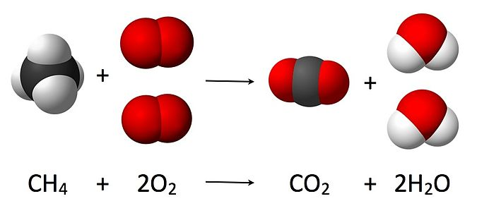
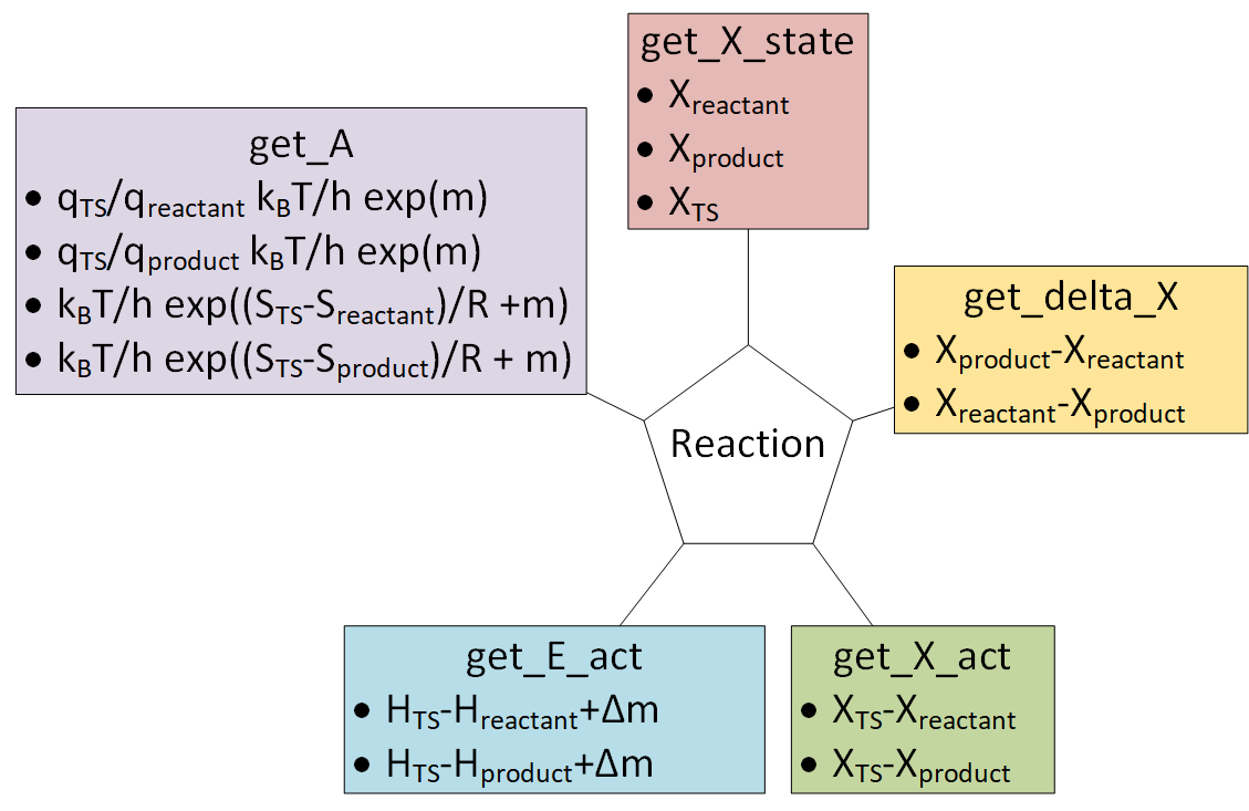
# # 6. Reactions
#
# ``Reaction`` objects can be created by putting together ``Nasa``, ``Nasa9``, ``Shomate`` and ``StatMech`` objects.
#
#
# ## 4.1. Inputting a NASA polynomial directly
#
# The H2 NASA polynomial from the [Burcat database](http://combustion.berkeley.edu/gri_mech/version30/files30/thermo30.dat) is represented as:
#
# ```
# H2 TPIS78H 2 G 200.000 3500.000 1000.000 1
# 3.33727920E+00-4.94024731E-05 4.99456778E-07-1.79566394E-10 2.00255376E-14 2
# -9.50158922E+02-3.20502331E+00 2.34433112E+00 7.98052075E-03-1.94781510E-05 3
# 2.01572094E-08-7.37611761E-12-9.17935173E+02 6.83010238E-01 4
# ```
#
# This can be translated to pMuTT syntax using:
# In[5]:
import numpy as np
from matplotlib import pyplot as plt
from pmutt import plot_1D
from pmutt.empirical.nasa import Nasa
# Initialize NASA polynomial
H2_nasa = Nasa(name='H2',
elements={'H': 2},
phase='G',
T_low=200., T_mid=1000., T_high=3500.,
a_low=[2.34433112E+00, 7.98052075E-03, -1.94781510E-05,
2.01572094E-08, -7.37611761E-12, -9.17935173E+02,
6.83010238E-01],
a_high=[3.33727920E+00, -4.94024731E-05, 4.99456778E-07,
-1.79566394E-10, 2.00255376E-14, -9.50158922E+02,
-3.20502331E+00])
# Calculate thermodynamic quantities using the same syntax as StatMech
H_H2 = H2_nasa.get_H(units='kcal/mol', T=298.)
print('H_H2(T=298 K) = {} kcal/mol'.format(H_H2))
# Show thermodynamic quantities vs. T
T = np.linspace(200., 3500.)
f2, ax2 = plot_1D(H2_nasa,
x_name='T', x_values=T,
methods=('get_H', 'get_S', 'get_G'),
get_H_kwargs={'units': 'kcal/mol'},
get_S_kwargs={'units': 'cal/mol/K'},
get_G_kwargs={'units': 'kcal/mol'})
# Modifying figure
ax2[0].set_ylabel('H (kcal/mol)')
ax2[1].set_ylabel('S (cal/mol/K)')
ax2[2].set_ylabel('G (kcal/mol)')
ax2[2].set_xlabel('T (K)')
f2.set_size_inches(5, 5)
f2.set_dpi(200)
plt.show()
#
# ## 4.2. Fitting an empirical object to a StatMech object
# Empirical objects can be made directly any species objects using the ``from_model`` method.
# In[6]:
H2_nasa = Nasa.from_model(name='H2',
T_low=200.,
T_high=3500.,
model=H2_statmech)
# Compare the statistical mechanical model to the empirical model
f3, ax3 = H2_nasa.plot_statmech_and_empirical(Cp_units='J/mol/K',
H_units='kJ/mol',
S_units='J/mol/K',
G_units='kJ/mol')
f3.set_size_inches(6, 8)
f3.set_dpi(150)
plt.show()
# In[7]:
from pmutt.empirical.shomate import Shomate
H2_shomate = Shomate.from_model(model=H2_nasa)
# Compare the statistical mechanical model to the empirical model
f3, ax3 = H2_shomate.plot_statmech_and_empirical(Cp_units='J/mol/K',
H_units='kJ/mol',
S_units='J/mol/K',
G_units='kJ/mol')
f3.set_size_inches(6, 8)
f3.set_dpi(150)
plt.show()
# The ``Shomate`` is a simpler polynomial than the ``Nasa`` polynomial so it does not capture the features as well for the large T range. It is always a good idea to check your fit.
#
# # 5. Input/Output
# pMuTT has more IO functionality than below. See this page for [supported IO functions](https://vlachosgroup.github.io/pMuTT/io.html).
#
# ## 5.1. Input via Excel
#
# Encoding each object in Python can be tedious. You can read several species from Excel spreadsheets using [``pmutt.io.excel.read_excel``](https://vlachosgroup.github.io/pmutt/io.html?highlight=read_excel#pmutt.io.excel.read_excel). Note that this function returns a list of dictionaries. This output allows you to initialize whichever object you want using kwargs syntax. There are also [special rules that depend on the header name](https://vlachosgroup.github.io/pMuTT/io.html#special-rules).
#
# Below, we show an example importing species data from a spreadsheet and creating a series of NASA polynomials.
# First, we ensure that the current working directory is the same as the notebook so we can access the spreadsheet.
# In[8]:
import os
from pathlib import Path
# Find the location of Jupyter notebook
# Note that normally Python scripts have a __file__ variable but Jupyter notebook doesn't.
# Using pathlib can overcome this limiation
try:
notebook_path = os.path.dirname(__file__)
except NameError:
notebook_path = Path().resolve()
os.chdir(notebook_path)
# Now we can read from the spreadsheet.
# In[9]:
from pprint import pprint
from pmutt.io.excel import read_excel
ab_initio_data = read_excel(io='./input/NH3_Input_Data.xlsx', sheet_name='species')
pprint(ab_initio_data)
# After the data is read, we can fit the ``Nasa`` objects from the statistical mechanical data.
# In[10]:
from pmutt.empirical.nasa import Nasa
# Create NASA polynomials using **kwargs syntax
nasa_species = []
for species_data in ab_initio_data:
single_nasa_species = Nasa.from_model(T_low=100.,
T_high=1500.,
**species_data)
nasa_species.append(single_nasa_species)
# Just to ensure the species were read correctly, we can try printing out thermodynamic values.
# In[11]:
import pandas as pd
thermo_data = {'Name': [],
'H (kcal/mol)': [],
'S (cal/mol/K)': [],
'G (kcal/mol)': []}
'''Calculate properties at 298 K'''
T = 298. # K
for single_nasa_species in nasa_species:
thermo_data['Name'].append(single_nasa_species.name)
thermo_data['H (kcal/mol)'].append(single_nasa_species.get_H(units='kcal/mol', T=T))
thermo_data['S (cal/mol/K)'].append(single_nasa_species.get_S(units='cal/mol/K', T=T))
thermo_data['G (kcal/mol)'].append(single_nasa_species.get_G(units='kcal/mol', T=T))
'''Create Pandas Dataframe for easy printing'''
columns = ['Name', 'H (kcal/mol)', 'S (cal/mol/K)', 'G (kcal/mol)']
thermo_data = pd.DataFrame(thermo_data, columns=columns)
print(thermo_data)
#
# # 6. Reactions
#
# ``Reaction`` objects can be created by putting together ``Nasa``, ``Nasa9``, ``Shomate`` and ``StatMech`` objects.
#  #
#
#
#  #
#
#
#  #
# ## 6.1. Initializing Reaction objects using from_string
#
# The ``from_string`` method is the easiest way to create a ``Reaction`` object. It requires the relevant species to be in a dictionary and a string to describe the reaction.
#
#
#
# ## 6.1. Initializing Reaction objects using from_string
#
# The ``from_string`` method is the easiest way to create a ``Reaction`` object. It requires the relevant species to be in a dictionary and a string to describe the reaction.
#
#  #
# We will demonstrate its use for the formation of NH3.
# In[12]:
from pmutt.empirical.nasa import Nasa
from pmutt.empirical.shomate import Shomate
from pmutt.reaction import Reaction
# Create species. Note that you can mix different types of species
species = {
'H2': StatMech(name='H2', atoms=molecule('H2'),
vib_wavenumbers=[4342.], # cm-1
symmetrynumber=2,
potentialenergy=-6.77, # eV
spin=0.,
**presets['idealgas']),
'N2': Nasa(name='N2', T_low=300., T_mid=643., T_high=1000.,
a_low=[3.3956319945669633, 0.001115707689025668,
-4.301993779374381e-06, 6.8071424019295535e-09,
-3.2903312791047058e-12, -191001.55648623788,
3.556111439828502],
a_high=[4.050329990684662, -0.0029677854067980108,
5.323485005316287e-06, -3.3518122405333548e-09,
7.58446718337381e-13, -191086.2004520406,
0.6858235504924011]),
'NH3': Shomate(name='NH3', T_low=300., T_high=1000.,
a=[18.792357134351683, 44.82725349479501,
-10.05898449447048, 0.3711633831565547,
0.2969942466370908, -1791.225746924463,
203.9035662274934, 1784.714638346206]),
}
# Define the formation of ammonia reaction
rxn = Reaction.from_string('1.5H2 + 0.5N2 = NH3', species)
# Now we can calculate thermodynamic properties of the reaction.
# In[13]:
'''Forward change in enthalpy'''
H_rxn_fwd = rxn.get_delta_H(units='kcal/mol', T=300.)
print('Delta H_fwd(T = 300 K) = {:.1f} kcal/mol'.format(H_rxn_fwd))
'''Reverse change in entropy'''
S_rxn_rev = rxn.get_delta_S(units='cal/mol/K', T=300., rev=True)
print('Delta S_rev(T = 300 K) = {:.1f} cal/mol/K'.format(S_rxn_rev))
'''Gibbs energy of reactants'''
G_react = rxn.get_G_state(units='kcal/mol', T=300., state='reactants')
print('G_reactants(T = 300 K) = {:.1f} kcal/mol'.format(G_react))
#
# We will demonstrate its use for the formation of NH3.
# In[12]:
from pmutt.empirical.nasa import Nasa
from pmutt.empirical.shomate import Shomate
from pmutt.reaction import Reaction
# Create species. Note that you can mix different types of species
species = {
'H2': StatMech(name='H2', atoms=molecule('H2'),
vib_wavenumbers=[4342.], # cm-1
symmetrynumber=2,
potentialenergy=-6.77, # eV
spin=0.,
**presets['idealgas']),
'N2': Nasa(name='N2', T_low=300., T_mid=643., T_high=1000.,
a_low=[3.3956319945669633, 0.001115707689025668,
-4.301993779374381e-06, 6.8071424019295535e-09,
-3.2903312791047058e-12, -191001.55648623788,
3.556111439828502],
a_high=[4.050329990684662, -0.0029677854067980108,
5.323485005316287e-06, -3.3518122405333548e-09,
7.58446718337381e-13, -191086.2004520406,
0.6858235504924011]),
'NH3': Shomate(name='NH3', T_low=300., T_high=1000.,
a=[18.792357134351683, 44.82725349479501,
-10.05898449447048, 0.3711633831565547,
0.2969942466370908, -1791.225746924463,
203.9035662274934, 1784.714638346206]),
}
# Define the formation of ammonia reaction
rxn = Reaction.from_string('1.5H2 + 0.5N2 = NH3', species)
# Now we can calculate thermodynamic properties of the reaction.
# In[13]:
'''Forward change in enthalpy'''
H_rxn_fwd = rxn.get_delta_H(units='kcal/mol', T=300.)
print('Delta H_fwd(T = 300 K) = {:.1f} kcal/mol'.format(H_rxn_fwd))
'''Reverse change in entropy'''
S_rxn_rev = rxn.get_delta_S(units='cal/mol/K', T=300., rev=True)
print('Delta S_rev(T = 300 K) = {:.1f} cal/mol/K'.format(S_rxn_rev))
'''Gibbs energy of reactants'''
G_react = rxn.get_G_state(units='kcal/mol', T=300., state='reactants')
print('G_reactants(T = 300 K) = {:.1f} kcal/mol'.format(G_react))