#!/usr/bin/env python
# coding: utf-8
# # Overview of pMuTT's Core Functionality
# Originally written for Version 1.2.1
#
# Last Updated for Version 1.2.13
#
# ## Topics Covered
#
# - Using constants and converting units using the ``constants`` module
# - Initializing ``StatMech`` objects by specifying all modes and by using ``presets`` dictionary
# - Initializing empirical objects such as ``Nasa`` objects using a ``StatMech`` object or from a previously generated Nasa polynomial
# - Initializing ``Reference`` and ``References`` objects to adjust DFT's reference to more traditional references
# - Input (via Excel) and output ``Nasa`` polynomials to thermdat format
# - Initializing ``Reaction`` objects from strings
#
# ## Useful Links:
#
# - Github: https://github.com/VlachosGroup/pMuTT
# - Documentation: https://vlachosgroup.github.io/pMuTT/index.html
# - Examples: https://vlachosgroup.github.io/pMuTT/examples.html
# ## Constants
# pMuTT has a wide variety of constants to increase readability of the code. See [Constants page][0] in the documentation for supported units.
#
# [0]: https://vlachosgroup.github.io/pmutt/constants.html#constants
# In[1]:
from pmutt import constants as c
1.987
print(c.R('kJ/mol/K'))
print('Some constants')
print('R (J/mol/K) = {}'.format(c.R('J/mol/K')))
print("Avogadro's number = {}\n".format(c.Na))
print('Unit conversions')
print('5 kJ/mol --> {} eV/molecule'.format(c.convert_unit(num=5., initial='kJ/mol', final='eV/molecule')))
print('Frequency of 1000 Hz --> Wavenumber of {} 1/cm\n'.format(c.freq_to_wavenumber(1000.)))
print('See expected inputs, supported units of different constants')
help(c.R)
help(c.convert_unit)
# ## StatMech Objects
# Molecules show translational, vibrational, rotational, electronic, and nuclear modes.
#
# 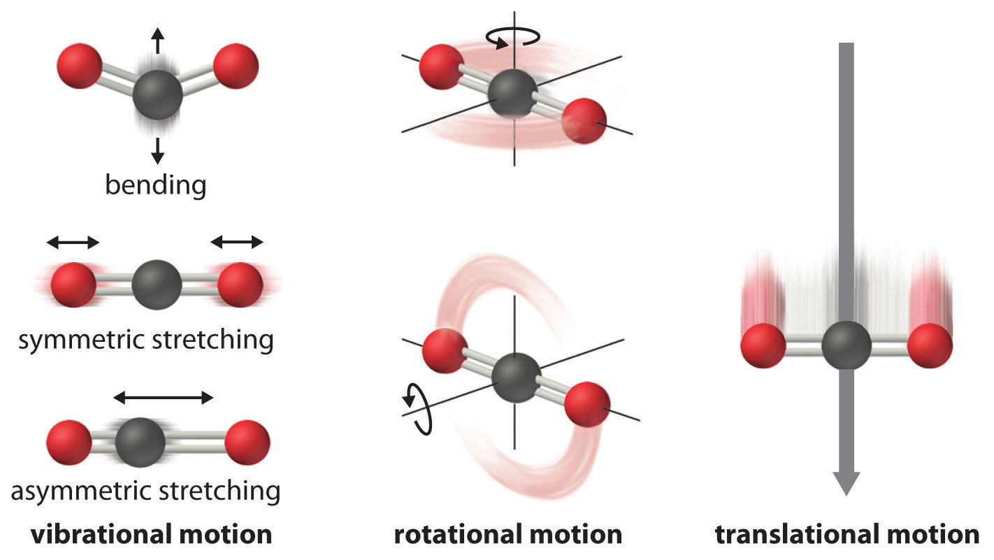 #
# The [``StatMech``][0] object allows us to specify translational, vibrational, rotational, electronic and nuclear modes independently, which gives flexibility in what behavior you would like.
#
# [0]: https://vlachosgroup.github.io/pmutt/statmech.html#pmutt.statmech.StatMech
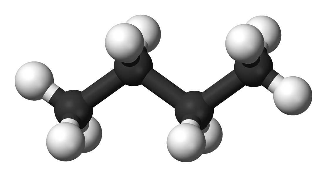
# For this example, we will use a butane molecule as an ideal gas:
#
# - translations with no interaction between molecules
# - harmonic vibrations
# - rigid rotor rotations
# - ground state electronic structure -
# - ground state nuclear structure).
#
#
#
# The [``StatMech``][0] object allows us to specify translational, vibrational, rotational, electronic and nuclear modes independently, which gives flexibility in what behavior you would like.
#
# [0]: https://vlachosgroup.github.io/pmutt/statmech.html#pmutt.statmech.StatMech
# For this example, we will use a butane molecule as an ideal gas:
#
# - translations with no interaction between molecules
# - harmonic vibrations
# - rigid rotor rotations
# - ground state electronic structure -
# - ground state nuclear structure).
#
#  # In[2]:
from ase.build import molecule
from pmutt.statmech import StatMech, trans, vib, rot, elec
butane_atoms = molecule('trans-butane')
'''Translational'''
butane_trans = trans.FreeTrans(n_degrees=3, atoms=butane_atoms)
'''Vibrational'''
butane_vib = vib.HarmonicVib(vib_wavenumbers=[3054.622862, 3047.573455, 3037.53448,
3030.21322, 3029.947329, 2995.758708,
2970.12166, 2968.142985, 2951.122942,
2871.560685, 1491.354921, 1456.480829,
1455.224163, 1429.084081, 1423.153673,
1364.456094, 1349.778994, 1321.137752,
1297.412109, 1276.969173, 1267.783512,
1150.401492, 1027.841298, 1018.203753,
945.310074, 929.15992, 911.661049,
808.685354, 730.986587, 475.287654,
339.164649, 264.682213, 244.584138,
219.956713, 115.923768, 35.56194])
'''Rotational'''
butane_rot = rot.RigidRotor(symmetrynumber=2, atoms=butane_atoms)
'''Electronic'''
butane_elec = elec.GroundStateElec(potentialenergy=-73.7051, spin=0)
'''StatMech Initialization'''
butane_statmech = StatMech(name='butane',
trans_model=butane_trans,
vib_model=butane_vib,
rot_model=butane_rot,
elec_model=butane_elec)
H_statmech = butane_statmech.get_H(T=298., units='kJ/mol')
S_statmech = butane_statmech.get_S(T=298., units='J/mol/K')
print('H_butane(T=298) = {:.1f} kJ/mol'.format(H_statmech))
print('S_butane(T=298) = {:.2f} J/mol/K'.format(S_statmech))
# ### Presets
# The [``presets``][0] dictionary stores commonly used models to ease the initialization of [``StatMech``][1] objects. The same water molecule before can be initialized this way instead.
#
# [0]: https://vlachosgroup.github.io/pmutt/statmech.html#presets
# [1]: https://vlachosgroup.github.io/pmutt/statmech.html#pmutt.statmech.StatMech
# In[3]:
from pprint import pprint
from ase.build import molecule
from pmutt.statmech import StatMech, presets
idealgas_defaults = presets['idealgas']
pprint(idealgas_defaults)
# In[4]:
butane_preset = StatMech(name='butane',
atoms=molecule('trans-butane'),
vib_wavenumbers=[3054.622862, 3047.573455, 3037.53448,
3030.21322, 3029.947329, 2995.758708,
2970.12166, 2968.142985, 2951.122942,
2871.560685, 1491.354921, 1456.480829,
1455.224163, 1429.084081, 1423.153673,
1364.456094, 1349.778994, 1321.137752,
1297.412109, 1276.969173, 1267.783512,
1150.401492, 1027.841298, 1018.203753,
945.310074, 929.15992, 911.661049,
808.685354, 730.986587, 475.287654,
339.164649, 264.682213, 244.584138,
219.956713, 115.923768, 35.56194],
symmetrynumber=2,
potentialenergy=-73.7051,
spin=0,
**idealgas_defaults)
H_preset = butane_preset.get_H(T=298., units='kJ/mol')
S_preset = butane_preset.get_S(T=298., units='J/mol/K')
print('H_butane(T=298) = {:.1f} kJ/mol'.format(H_preset))
print('S_butane(T=298) = {:.2f} J/mol/K'.format(S_preset))
# ### Empty Modes
# The [``EmptyMode``][0] is a special object returns 1 for the partition function and 0 for all other thermodynamic properties. This is useful if you do not want any contribution from a mode.
#
# [0]: https://vlachosgroup.github.io/pmutt/statmech.html#empty-mode
# In[5]:
from pmutt.statmech import EmptyMode
empty = EmptyMode()
print('Some EmptyMode properties:')
print('q = {}'.format(empty.get_q()))
print('H/RT = {}'.format(empty.get_HoRT()))
print('S/R = {}'.format(empty.get_SoR()))
print('G/RT = {}'.format(empty.get_GoRT()))
# ## Empirical Objects
# Empirical forms are polynomials that are fit to experimental or *ab-initio data*. These forms are useful because they can be evaluated relatively quickly, so that downstream software is not hindered by evaluation of thermochemical properties.
# However, note that ``StatMech`` objects can calculate more properties than the currently supported empirical objects.
# ### NASA polynomial
# The [``NASA``][0] format is used for our microkinetic modeling software, Chemkin.
#
# #### Initializing Nasa from StatMech
# Below, we initialize the NASA polynomial from the ``StatMech`` object we created earlier.
#
# [0]: https://vlachosgroup.github.io/pmutt/empirical.html#nasa
# In[6]:
from pmutt.empirical.nasa import Nasa
butane_nasa = Nasa.from_model(name='butane',
model=butane_statmech,
T_low=298.,
T_high=800.,
elements={'C': 4, 'H': 10},
phase='G')
H_nasa = butane_nasa.get_H(T=298., units='kJ/mol')
S_nasa = butane_nasa.get_S(T=298., units='J/mol/K')
print('H_butane(T=298) = {:.1f} kJ/mol'.format(H_nasa))
print('S_butane(T=298) = {:.2f} J/mol/K'.format(S_nasa))
# Although it is not covered here, you can also generate empirical objects from experimental data using the ``.from_data`` method. See [Experimental to Empirical][6] example.
#
# [6]: https://vlachosgroup.github.io/pmutt/examples.html#experimental-to-empirical
# #### Initializing Nasa Directly
# We can also initialize the NASA polynomial if we have the polynomials. Using an entry from the [Reaction Mechanism Generator (RMG) database][0].
#
# [0]: https://rmg.mit.edu/database/thermo/libraries/DFT_QCI_thermo/215/
# In[7]:
import numpy as np
butane_nasa_direct = Nasa(name='butane',
T_low=100.,
T_mid=1147.61,
T_high=5000.,
a_low=np.array([ 2.16917742E+00,
3.43905384E-02,
-1.61588593E-06,
-1.30723691E-08,
5.17339469E-12,
-1.72505133E+04,
1.46546944E+01]),
a_high=np.array([ 6.78908025E+00,
3.03597365E-02,
-1.21261608E-05,
2.19944009E-09,
-1.50288488E-13,
-1.91058191E+04,
-1.17331911E+01]),
elements={'C': 4, 'H': 10},
phase='G')
H_nasa_direct = butane_nasa_direct.get_H(T=298., units='kJ/mol')
S_nasa_direct = butane_nasa_direct.get_S(T=298., units='J/mol/K')
print('H_butane(T=298) = {:.1f} kJ/mol'.format(H_nasa_direct))
print('S_butane(T=298) = {:.2f} J/mol/K'.format(S_nasa_direct))
# Compare the results between ``butane_nasa`` and ``butane_nasa_direct`` to the [Wikipedia page for butane][0].
#
# [0]: https://en.wikipedia.org/wiki/Butane_(data_page)
# In[8]:
print('H_nasa = {:.1f} kJ/mol'.format(H_nasa))
print('H_nasa_direct = {:.1f} kJ/mol'.format(H_nasa_direct))
print('H_wiki = -125.6 kJ/mol\n')
print('S_nasa = {:.2f} J/mol/K'.format(S_nasa))
print('S_nasa_direct = {:.2f} J/mol/K'.format(S_nasa_direct))
print('S_wiki = 310.23 J/mol/K')
# Notice the values are very different for ``H_nasa``. This discrepancy is due to:
#
# - different references
# - error in DFT
#
# We can account for this discrepancy by using the [``Reference``][0] and [``References``][1] objects.
#
# [0]: https://vlachosgroup.github.io/pmutt/empirical.html#pmutt.empirical.references.Reference
# [1]: https://vlachosgroup.github.io/pmutt/empirical.html#pmutt.empirical.references.References
# ### Referencing
# To define a reference, you must have:
#
# - enthalpy at some reference temperature (``HoRT_ref`` and ``T_ref``)
# - a ``StatMech`` object
#
# In general, use references that are similar to molecules in your mechanism. Also, the number of reference molecules must be equation to the number of elements (or other descriptor) in the mechanism. [Full description of referencing scheme here][0].
#
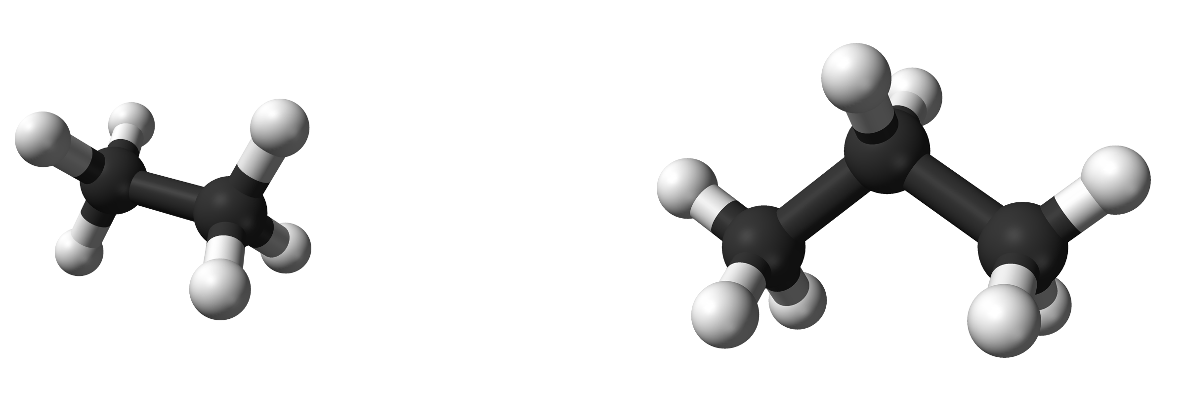
# In this example, we will use ethane and propane as references.
#
#
# In[2]:
from ase.build import molecule
from pmutt.statmech import StatMech, trans, vib, rot, elec
butane_atoms = molecule('trans-butane')
'''Translational'''
butane_trans = trans.FreeTrans(n_degrees=3, atoms=butane_atoms)
'''Vibrational'''
butane_vib = vib.HarmonicVib(vib_wavenumbers=[3054.622862, 3047.573455, 3037.53448,
3030.21322, 3029.947329, 2995.758708,
2970.12166, 2968.142985, 2951.122942,
2871.560685, 1491.354921, 1456.480829,
1455.224163, 1429.084081, 1423.153673,
1364.456094, 1349.778994, 1321.137752,
1297.412109, 1276.969173, 1267.783512,
1150.401492, 1027.841298, 1018.203753,
945.310074, 929.15992, 911.661049,
808.685354, 730.986587, 475.287654,
339.164649, 264.682213, 244.584138,
219.956713, 115.923768, 35.56194])
'''Rotational'''
butane_rot = rot.RigidRotor(symmetrynumber=2, atoms=butane_atoms)
'''Electronic'''
butane_elec = elec.GroundStateElec(potentialenergy=-73.7051, spin=0)
'''StatMech Initialization'''
butane_statmech = StatMech(name='butane',
trans_model=butane_trans,
vib_model=butane_vib,
rot_model=butane_rot,
elec_model=butane_elec)
H_statmech = butane_statmech.get_H(T=298., units='kJ/mol')
S_statmech = butane_statmech.get_S(T=298., units='J/mol/K')
print('H_butane(T=298) = {:.1f} kJ/mol'.format(H_statmech))
print('S_butane(T=298) = {:.2f} J/mol/K'.format(S_statmech))
# ### Presets
# The [``presets``][0] dictionary stores commonly used models to ease the initialization of [``StatMech``][1] objects. The same water molecule before can be initialized this way instead.
#
# [0]: https://vlachosgroup.github.io/pmutt/statmech.html#presets
# [1]: https://vlachosgroup.github.io/pmutt/statmech.html#pmutt.statmech.StatMech
# In[3]:
from pprint import pprint
from ase.build import molecule
from pmutt.statmech import StatMech, presets
idealgas_defaults = presets['idealgas']
pprint(idealgas_defaults)
# In[4]:
butane_preset = StatMech(name='butane',
atoms=molecule('trans-butane'),
vib_wavenumbers=[3054.622862, 3047.573455, 3037.53448,
3030.21322, 3029.947329, 2995.758708,
2970.12166, 2968.142985, 2951.122942,
2871.560685, 1491.354921, 1456.480829,
1455.224163, 1429.084081, 1423.153673,
1364.456094, 1349.778994, 1321.137752,
1297.412109, 1276.969173, 1267.783512,
1150.401492, 1027.841298, 1018.203753,
945.310074, 929.15992, 911.661049,
808.685354, 730.986587, 475.287654,
339.164649, 264.682213, 244.584138,
219.956713, 115.923768, 35.56194],
symmetrynumber=2,
potentialenergy=-73.7051,
spin=0,
**idealgas_defaults)
H_preset = butane_preset.get_H(T=298., units='kJ/mol')
S_preset = butane_preset.get_S(T=298., units='J/mol/K')
print('H_butane(T=298) = {:.1f} kJ/mol'.format(H_preset))
print('S_butane(T=298) = {:.2f} J/mol/K'.format(S_preset))
# ### Empty Modes
# The [``EmptyMode``][0] is a special object returns 1 for the partition function and 0 for all other thermodynamic properties. This is useful if you do not want any contribution from a mode.
#
# [0]: https://vlachosgroup.github.io/pmutt/statmech.html#empty-mode
# In[5]:
from pmutt.statmech import EmptyMode
empty = EmptyMode()
print('Some EmptyMode properties:')
print('q = {}'.format(empty.get_q()))
print('H/RT = {}'.format(empty.get_HoRT()))
print('S/R = {}'.format(empty.get_SoR()))
print('G/RT = {}'.format(empty.get_GoRT()))
# ## Empirical Objects
# Empirical forms are polynomials that are fit to experimental or *ab-initio data*. These forms are useful because they can be evaluated relatively quickly, so that downstream software is not hindered by evaluation of thermochemical properties.
# However, note that ``StatMech`` objects can calculate more properties than the currently supported empirical objects.
# ### NASA polynomial
# The [``NASA``][0] format is used for our microkinetic modeling software, Chemkin.
#
# #### Initializing Nasa from StatMech
# Below, we initialize the NASA polynomial from the ``StatMech`` object we created earlier.
#
# [0]: https://vlachosgroup.github.io/pmutt/empirical.html#nasa
# In[6]:
from pmutt.empirical.nasa import Nasa
butane_nasa = Nasa.from_model(name='butane',
model=butane_statmech,
T_low=298.,
T_high=800.,
elements={'C': 4, 'H': 10},
phase='G')
H_nasa = butane_nasa.get_H(T=298., units='kJ/mol')
S_nasa = butane_nasa.get_S(T=298., units='J/mol/K')
print('H_butane(T=298) = {:.1f} kJ/mol'.format(H_nasa))
print('S_butane(T=298) = {:.2f} J/mol/K'.format(S_nasa))
# Although it is not covered here, you can also generate empirical objects from experimental data using the ``.from_data`` method. See [Experimental to Empirical][6] example.
#
# [6]: https://vlachosgroup.github.io/pmutt/examples.html#experimental-to-empirical
# #### Initializing Nasa Directly
# We can also initialize the NASA polynomial if we have the polynomials. Using an entry from the [Reaction Mechanism Generator (RMG) database][0].
#
# [0]: https://rmg.mit.edu/database/thermo/libraries/DFT_QCI_thermo/215/
# In[7]:
import numpy as np
butane_nasa_direct = Nasa(name='butane',
T_low=100.,
T_mid=1147.61,
T_high=5000.,
a_low=np.array([ 2.16917742E+00,
3.43905384E-02,
-1.61588593E-06,
-1.30723691E-08,
5.17339469E-12,
-1.72505133E+04,
1.46546944E+01]),
a_high=np.array([ 6.78908025E+00,
3.03597365E-02,
-1.21261608E-05,
2.19944009E-09,
-1.50288488E-13,
-1.91058191E+04,
-1.17331911E+01]),
elements={'C': 4, 'H': 10},
phase='G')
H_nasa_direct = butane_nasa_direct.get_H(T=298., units='kJ/mol')
S_nasa_direct = butane_nasa_direct.get_S(T=298., units='J/mol/K')
print('H_butane(T=298) = {:.1f} kJ/mol'.format(H_nasa_direct))
print('S_butane(T=298) = {:.2f} J/mol/K'.format(S_nasa_direct))
# Compare the results between ``butane_nasa`` and ``butane_nasa_direct`` to the [Wikipedia page for butane][0].
#
# [0]: https://en.wikipedia.org/wiki/Butane_(data_page)
# In[8]:
print('H_nasa = {:.1f} kJ/mol'.format(H_nasa))
print('H_nasa_direct = {:.1f} kJ/mol'.format(H_nasa_direct))
print('H_wiki = -125.6 kJ/mol\n')
print('S_nasa = {:.2f} J/mol/K'.format(S_nasa))
print('S_nasa_direct = {:.2f} J/mol/K'.format(S_nasa_direct))
print('S_wiki = 310.23 J/mol/K')
# Notice the values are very different for ``H_nasa``. This discrepancy is due to:
#
# - different references
# - error in DFT
#
# We can account for this discrepancy by using the [``Reference``][0] and [``References``][1] objects.
#
# [0]: https://vlachosgroup.github.io/pmutt/empirical.html#pmutt.empirical.references.Reference
# [1]: https://vlachosgroup.github.io/pmutt/empirical.html#pmutt.empirical.references.References
# ### Referencing
# To define a reference, you must have:
#
# - enthalpy at some reference temperature (``HoRT_ref`` and ``T_ref``)
# - a ``StatMech`` object
#
# In general, use references that are similar to molecules in your mechanism. Also, the number of reference molecules must be equation to the number of elements (or other descriptor) in the mechanism. [Full description of referencing scheme here][0].
#
# In this example, we will use ethane and propane as references.
#
#  #
# [0]: https://vlachosgroup.github.io/pmutt/referencing.html
# In[9]:
from pmutt.empirical.references import Reference, References
ethane_ref = Reference(name='ethane',
elements={'C': 2, 'H': 6},
atoms=molecule('C2H6'),
vib_wavenumbers=[3050.5296, 3049.8428, 3025.2714,
3024.4304, 2973.5455, 2971.9261,
1455.4203, 1454.9941, 1454.2055,
1453.7038, 1372.4786, 1358.3593,
1176.4512, 1175.507, 992.55,
803.082, 801.4536, 298.4712],
symmetrynumber=6,
potentialenergy=-40.5194,
spin=0,
T_ref=298.15,
HoRT_ref=-33.7596,
**idealgas_defaults)
propane_ref = Reference(name='propane',
elements={'C': 3, 'H': 8},
atoms=molecule('C3H8'),
vib_wavenumbers=[3040.9733, 3038.992, 3036.8071,
3027.6062, 2984.8436, 2966.1692,
2963.4684, 2959.7431, 1462.5683,
1457.4221, 1446.858, 1442.0357,
1438.7871, 1369.6901, 1352.6287,
1316.215, 1273.9426, 1170.4456,
1140.9699, 1049.3866, 902.8507,
885.3209, 865.5958, 735.1924,
362.7372, 266.3928, 221.4547],
symmetrynumber=2,
potentialenergy=-57.0864,
spin=0,
T_ref=298.15,
HoRT_ref=-42.2333,
**idealgas_defaults)
refs = References(references=[ethane_ref, propane_ref])
print(refs.offset)
# Passing the ``References`` object when we make our ``Nasa`` object produces a value closer to the one listed above.
# In[10]:
butane_nasa_ref = Nasa.from_model(name='butane',
model=butane_statmech,
T_low=298.,
T_high=800.,
elements={'C': 4, 'H': 10},
references=refs)
H_nasa_ref = butane_nasa_ref.get_H(T=298., units='kJ/mol')
S_nasa_ref = butane_nasa_ref.get_S(T=298., units='J/mol/K')
print('H_butane(T=298) = {:.1f} kJ/mol'.format(H_nasa_ref))
print('S_butane(T=298) = {:.2f} J/mol/K'.format(S_nasa_ref))
# ## Input and Output
# ### Excel
# Encoding each object in Python can be tedious and so you can read from Excel spreadsheets using [``pmutt.io.excel.read_excel``][0]. Note that this function returns a list of dictionaries. This output allows you to initialize whichever object you want. There are also special rules that depend on the header name.
#
# [0]: https://vlachosgroup.github.io/pmutt/io.html?highlight=read_excel#pmutt.io.excel.read_excel
# In[11]:
import os
from pathlib import Path
from pmutt.io.excel import read_excel
# Find the location of Jupyter notebook
# Note that normally Python scripts have a __file__ variable but Jupyter notebook doesn't.
# Using pathlib can overcome this limiation
try:
notebook_folder = os.path.dirname(__file__)
except NameError:
notebook_folder = Path().resolve()
os.chdir(notebook_folder)
# The Excel spreadsheet is located in the same folder as the Jupyter notebook
refs_path = os.path.join(notebook_folder, 'refs.xlsx')
refs_data = read_excel(refs_path)
pprint(refs_data)
# Initialize using \*\*kwargs syntax.
# In[12]:
ref_list = []
for record in refs_data:
ref_list.append(Reference(**record))
refs_excel = References(references=ref_list)
print(refs_excel.offset)
# Butane can be initialized in a similar way.
# In[13]:
# The Excel spreadsheet is located in the same folder as the Jupyter notebook
butane_path = os.path.join(notebook_folder, 'butane.xlsx')
butane_data = read_excel(butane_path)[0] # [0] accesses the butane data
butane_excel = Nasa.from_model(T_low=298.,
T_high=800.,
references=refs_excel,
**butane_data)
H_excel = butane_excel.get_H(T=298., units='kJ/mol')
S_excel = butane_excel.get_S(T=298., units='J/mol/K')
print('H_butane(T=298) = {:.1f} kJ/mol'.format(H_excel))
print('S_butane(T=298) = {:.2f} J/mol/K'.format(S_excel))
# ### Thermdat
# The thermdat format uses NASA polynomials to represent several species. It has a very particular format so doing it manually is error-prone. You can write a list of ``Nasa`` objects to thermdat format using [``pmutt.io.thermdat.write_thermdat``][0].
#
# [0]: https://vlachosgroup.github.io/pmutt/io.html#pmutt.io.thermdat.write_thermdat
# In[14]:
from pmutt.io.thermdat import write_thermdat
# Make Nasa objects from previously defined ethane and propane
ethane_nasa = Nasa.from_model(name='ethane',
phase='G',
T_low=298.,
T_high=800.,
model=ethane_ref.model,
elements=ethane_ref.elements,
references=refs)
propane_nasa = Nasa.from_model(name='propane',
phase='G',
T_low=298.,
T_high=800.,
model=propane_ref.model,
elements=propane_ref.elements,
references=refs)
nasa_species = [ethane_nasa, propane_nasa, butane_nasa]
# Determine the output path and write the thermdat file
thermdat_path = os.path.join(notebook_folder, 'thermdat')
write_thermdat(filename=thermdat_path, nasa_species=nasa_species)
THERMO ALL
100 500 1500
ethane 20190122C 2H 6 G298.0 800.0 502.9 1
-6.84729317E-01 2.54150584E-02-1.02900193E-05-1.15304090E-09 1.73800327E-12 2
-1.08866341E+04 2.42655635E+01 6.77655563E+00-3.31037518E-02 1.63456769E-04 3
-2.32569163E-07 1.18361103E-10-1.16548936E+04-6.74224205E+00 4
propane 20190122C 3H 8 G298.0 800.0 502.9 1
-2.54716915E+00 4.36640749E-02-2.65978975E-05 6.89956646E-09 7.68567634E-14 2
-1.35353831E+04 3.50227651E+01 8.09253651E+00-4.01657054E-02 2.23439464E-04 3
-3.27632587E-07 1.69405578E-10-1.46259783E+04-9.14554121E+00 4
butane 20190122C 4H 10 G298.0 800.0 502.9 1
-1.98482876E+00 5.99910769E-02-4.67983727E-05 2.14853318E-08-4.31005098E-12 2
-8.15415828E+05 3.48691129E+01 9.98107805E+00-3.50556935E-02 2.38938732E-04 3
-3.63709779E-07 1.92062158E-10-8.16632302E+05-1.47065846E+01 4
END
# Similarly, [``pmutt.io.thermdat.read_thermdat``][0] reads thermdat files.
#
# [0]: https://vlachosgroup.github.io/pmutt/io.html#pmutt.io.thermdat.read_thermdat
# ## Reactions
# You can also evaluate reactions properties. The most straightforward way to do this is to initialize using strings.
# In[15]:
from pmutt.io.thermdat import read_thermdat
from pmutt import pmutt_list_to_dict
from pmutt.reaction import Reaction
# Get a dictionary of species
thermdat_H2O_path = os.path.join(notebook_folder, 'thermdat_H2O')
species_list = read_thermdat(thermdat_H2O_path)
species_dict = pmutt_list_to_dict(species_list)
# Initialize the reaction
rxn_H2O = Reaction.from_string('H2 + 0.5O2 = H2O', species=species_dict)
# Calculate reaction properties
H_rxn = rxn_H2O.get_delta_H(T=298., units='kJ/mol')
S_rxn = rxn_H2O.get_delta_S(T=298., units='J/mol/K')
print('H_rxn(T=298) = {:.1f} kJ/mol'.format(H_rxn))
print('S_rxn(T=298) = {:.2f} J/mol/K'.format(S_rxn))
# ## Exercise
# Write a script to calculate the Enthalpy of adsorption (in kcal/mol) of H2O on Cu(111) at T = 298 K. Some important details are given below.
#
# ### Information Required
# #### H2O:
# - ideal gas
# - atoms: You can use "ase.build.molecule" to generate a water molecule like we did with ethane, propane, and butane.
# - vibrational wavenumbers (1/cm): 3825.434, 3710.2642, 1582.432
# - potential energy (eV): -14.22393533
# - spin: 0
# - symmetry number: 2
#
# #### Cu(111):
# - only electronic modes
# - potential energy (eV): -224.13045381
#
# #### H2O+Cu(111):
# - electronic and harmonic vibration modes
# - potential energy (eV): -238.4713854
# - vibrational wavenumbers (1/cm): 3797.255519, 3658.895695, 1530.600295, 266.366130, 138.907356, 63.899768, 59.150454, 51.256019, -327.384554 (negative numbers represent imaginary frequencies. The default behavior of pMuTT is to ignore these frequencies when calculating any thermodynamic property)
#
# #### Reaction:
# H2O + Cu(111) --> H2O+Cu(111)
#
# ### Solution:
# In[16]:
from ase.build import molecule
from pmutt.statmech import StatMech, presets
from pmutt.reaction import Reaction
# Using dictionary since later I will initialize the reaction with a string
species = {
'H2O(g)': StatMech(atoms=molecule('H2O'),
vib_wavenumbers=[3825.434, 3710.2642, 1582.432],
potentialenergy=-14.22393533,
spin=0,
symmetrynumber=2,
**presets['idealgas']),
'*': StatMech(potentialenergy=-224.13045381,
**presets['electronic']),
'H2O*': StatMech(potentialenergy=-238.4713854,
vib_wavenumbers=[3797.255519,
3658.895695,
1530.600295,
266.366130,
138.907356,
63.899768,
59.150454,
51.256019,
-327.384554], #Imaginary frequency!
**presets['harmonic']),
}
rxn = Reaction.from_string('H2O(g) + * = H2O*', species)
del_H = rxn.get_delta_H(T=298., units='kcal/mol')
print('del_H = {:.2f} kcal/mol'.format(del_H))
# In[ ]:
#
# [0]: https://vlachosgroup.github.io/pmutt/referencing.html
# In[9]:
from pmutt.empirical.references import Reference, References
ethane_ref = Reference(name='ethane',
elements={'C': 2, 'H': 6},
atoms=molecule('C2H6'),
vib_wavenumbers=[3050.5296, 3049.8428, 3025.2714,
3024.4304, 2973.5455, 2971.9261,
1455.4203, 1454.9941, 1454.2055,
1453.7038, 1372.4786, 1358.3593,
1176.4512, 1175.507, 992.55,
803.082, 801.4536, 298.4712],
symmetrynumber=6,
potentialenergy=-40.5194,
spin=0,
T_ref=298.15,
HoRT_ref=-33.7596,
**idealgas_defaults)
propane_ref = Reference(name='propane',
elements={'C': 3, 'H': 8},
atoms=molecule('C3H8'),
vib_wavenumbers=[3040.9733, 3038.992, 3036.8071,
3027.6062, 2984.8436, 2966.1692,
2963.4684, 2959.7431, 1462.5683,
1457.4221, 1446.858, 1442.0357,
1438.7871, 1369.6901, 1352.6287,
1316.215, 1273.9426, 1170.4456,
1140.9699, 1049.3866, 902.8507,
885.3209, 865.5958, 735.1924,
362.7372, 266.3928, 221.4547],
symmetrynumber=2,
potentialenergy=-57.0864,
spin=0,
T_ref=298.15,
HoRT_ref=-42.2333,
**idealgas_defaults)
refs = References(references=[ethane_ref, propane_ref])
print(refs.offset)
# Passing the ``References`` object when we make our ``Nasa`` object produces a value closer to the one listed above.
# In[10]:
butane_nasa_ref = Nasa.from_model(name='butane',
model=butane_statmech,
T_low=298.,
T_high=800.,
elements={'C': 4, 'H': 10},
references=refs)
H_nasa_ref = butane_nasa_ref.get_H(T=298., units='kJ/mol')
S_nasa_ref = butane_nasa_ref.get_S(T=298., units='J/mol/K')
print('H_butane(T=298) = {:.1f} kJ/mol'.format(H_nasa_ref))
print('S_butane(T=298) = {:.2f} J/mol/K'.format(S_nasa_ref))
# ## Input and Output
# ### Excel
# Encoding each object in Python can be tedious and so you can read from Excel spreadsheets using [``pmutt.io.excel.read_excel``][0]. Note that this function returns a list of dictionaries. This output allows you to initialize whichever object you want. There are also special rules that depend on the header name.
#
# [0]: https://vlachosgroup.github.io/pmutt/io.html?highlight=read_excel#pmutt.io.excel.read_excel
# In[11]:
import os
from pathlib import Path
from pmutt.io.excel import read_excel
# Find the location of Jupyter notebook
# Note that normally Python scripts have a __file__ variable but Jupyter notebook doesn't.
# Using pathlib can overcome this limiation
try:
notebook_folder = os.path.dirname(__file__)
except NameError:
notebook_folder = Path().resolve()
os.chdir(notebook_folder)
# The Excel spreadsheet is located in the same folder as the Jupyter notebook
refs_path = os.path.join(notebook_folder, 'refs.xlsx')
refs_data = read_excel(refs_path)
pprint(refs_data)
# Initialize using \*\*kwargs syntax.
# In[12]:
ref_list = []
for record in refs_data:
ref_list.append(Reference(**record))
refs_excel = References(references=ref_list)
print(refs_excel.offset)
# Butane can be initialized in a similar way.
# In[13]:
# The Excel spreadsheet is located in the same folder as the Jupyter notebook
butane_path = os.path.join(notebook_folder, 'butane.xlsx')
butane_data = read_excel(butane_path)[0] # [0] accesses the butane data
butane_excel = Nasa.from_model(T_low=298.,
T_high=800.,
references=refs_excel,
**butane_data)
H_excel = butane_excel.get_H(T=298., units='kJ/mol')
S_excel = butane_excel.get_S(T=298., units='J/mol/K')
print('H_butane(T=298) = {:.1f} kJ/mol'.format(H_excel))
print('S_butane(T=298) = {:.2f} J/mol/K'.format(S_excel))
# ### Thermdat
# The thermdat format uses NASA polynomials to represent several species. It has a very particular format so doing it manually is error-prone. You can write a list of ``Nasa`` objects to thermdat format using [``pmutt.io.thermdat.write_thermdat``][0].
#
# [0]: https://vlachosgroup.github.io/pmutt/io.html#pmutt.io.thermdat.write_thermdat
# In[14]:
from pmutt.io.thermdat import write_thermdat
# Make Nasa objects from previously defined ethane and propane
ethane_nasa = Nasa.from_model(name='ethane',
phase='G',
T_low=298.,
T_high=800.,
model=ethane_ref.model,
elements=ethane_ref.elements,
references=refs)
propane_nasa = Nasa.from_model(name='propane',
phase='G',
T_low=298.,
T_high=800.,
model=propane_ref.model,
elements=propane_ref.elements,
references=refs)
nasa_species = [ethane_nasa, propane_nasa, butane_nasa]
# Determine the output path and write the thermdat file
thermdat_path = os.path.join(notebook_folder, 'thermdat')
write_thermdat(filename=thermdat_path, nasa_species=nasa_species)
THERMO ALL
100 500 1500
ethane 20190122C 2H 6 G298.0 800.0 502.9 1
-6.84729317E-01 2.54150584E-02-1.02900193E-05-1.15304090E-09 1.73800327E-12 2
-1.08866341E+04 2.42655635E+01 6.77655563E+00-3.31037518E-02 1.63456769E-04 3
-2.32569163E-07 1.18361103E-10-1.16548936E+04-6.74224205E+00 4
propane 20190122C 3H 8 G298.0 800.0 502.9 1
-2.54716915E+00 4.36640749E-02-2.65978975E-05 6.89956646E-09 7.68567634E-14 2
-1.35353831E+04 3.50227651E+01 8.09253651E+00-4.01657054E-02 2.23439464E-04 3
-3.27632587E-07 1.69405578E-10-1.46259783E+04-9.14554121E+00 4
butane 20190122C 4H 10 G298.0 800.0 502.9 1
-1.98482876E+00 5.99910769E-02-4.67983727E-05 2.14853318E-08-4.31005098E-12 2
-8.15415828E+05 3.48691129E+01 9.98107805E+00-3.50556935E-02 2.38938732E-04 3
-3.63709779E-07 1.92062158E-10-8.16632302E+05-1.47065846E+01 4
END
# Similarly, [``pmutt.io.thermdat.read_thermdat``][0] reads thermdat files.
#
# [0]: https://vlachosgroup.github.io/pmutt/io.html#pmutt.io.thermdat.read_thermdat
# ## Reactions
# You can also evaluate reactions properties. The most straightforward way to do this is to initialize using strings.
# In[15]:
from pmutt.io.thermdat import read_thermdat
from pmutt import pmutt_list_to_dict
from pmutt.reaction import Reaction
# Get a dictionary of species
thermdat_H2O_path = os.path.join(notebook_folder, 'thermdat_H2O')
species_list = read_thermdat(thermdat_H2O_path)
species_dict = pmutt_list_to_dict(species_list)
# Initialize the reaction
rxn_H2O = Reaction.from_string('H2 + 0.5O2 = H2O', species=species_dict)
# Calculate reaction properties
H_rxn = rxn_H2O.get_delta_H(T=298., units='kJ/mol')
S_rxn = rxn_H2O.get_delta_S(T=298., units='J/mol/K')
print('H_rxn(T=298) = {:.1f} kJ/mol'.format(H_rxn))
print('S_rxn(T=298) = {:.2f} J/mol/K'.format(S_rxn))
# ## Exercise
# Write a script to calculate the Enthalpy of adsorption (in kcal/mol) of H2O on Cu(111) at T = 298 K. Some important details are given below.
#
# ### Information Required
# #### H2O:
# - ideal gas
# - atoms: You can use "ase.build.molecule" to generate a water molecule like we did with ethane, propane, and butane.
# - vibrational wavenumbers (1/cm): 3825.434, 3710.2642, 1582.432
# - potential energy (eV): -14.22393533
# - spin: 0
# - symmetry number: 2
#
# #### Cu(111):
# - only electronic modes
# - potential energy (eV): -224.13045381
#
# #### H2O+Cu(111):
# - electronic and harmonic vibration modes
# - potential energy (eV): -238.4713854
# - vibrational wavenumbers (1/cm): 3797.255519, 3658.895695, 1530.600295, 266.366130, 138.907356, 63.899768, 59.150454, 51.256019, -327.384554 (negative numbers represent imaginary frequencies. The default behavior of pMuTT is to ignore these frequencies when calculating any thermodynamic property)
#
# #### Reaction:
# H2O + Cu(111) --> H2O+Cu(111)
#
# ### Solution:
# In[16]:
from ase.build import molecule
from pmutt.statmech import StatMech, presets
from pmutt.reaction import Reaction
# Using dictionary since later I will initialize the reaction with a string
species = {
'H2O(g)': StatMech(atoms=molecule('H2O'),
vib_wavenumbers=[3825.434, 3710.2642, 1582.432],
potentialenergy=-14.22393533,
spin=0,
symmetrynumber=2,
**presets['idealgas']),
'*': StatMech(potentialenergy=-224.13045381,
**presets['electronic']),
'H2O*': StatMech(potentialenergy=-238.4713854,
vib_wavenumbers=[3797.255519,
3658.895695,
1530.600295,
266.366130,
138.907356,
63.899768,
59.150454,
51.256019,
-327.384554], #Imaginary frequency!
**presets['harmonic']),
}
rxn = Reaction.from_string('H2O(g) + * = H2O*', species)
del_H = rxn.get_delta_H(T=298., units='kcal/mol')
print('del_H = {:.2f} kcal/mol'.format(del_H))
# In[ ]: