# nature-figure skill
Submission-grade scientific figures for Nature-tier journals and high-impact academic venues,
with both Python and R plotting tracks.
The skill starts from a figure contract: core conclusion, evidence hierarchy, archetype,
backend choice, journal/export constraints, statistics, and source-data traceability.
Plotting templates are used only after the scientific logic is clear.
Python remains the best-supported low-level layout path through `matplotlib`, `seaborn`,
`subplot_mosaic`, and `statsmodels`. R is supported through `ggplot2`, `patchwork`,
`ComplexHeatmap`, `ggrepel`, `svglite`, `cairo_pdf`, and `ragg`. If private template
collections are used, their paths, filenames, and provenance must not appear in
user-facing output.
Derived from production scripts in [figures4papers](https://github.com/ChenLiu-1996/figures4papers)
(published in *Nature Machine Intelligence* and top ML/bioinformatics venues).
---
## Example output gallery
The images below are simulated data mockups generated with this skill's rules:
editable SVG-first export, restrained semantic palettes, lowercase panel labels, and
asymmetric multi-panel information architecture. They are PNG previews for README display;
production use should still export SVG/PDF from the plotting script.
| Figure | Preview | What the skill demonstrates |
|--------|---------|-----------------------------|
| Material design and physical validation | 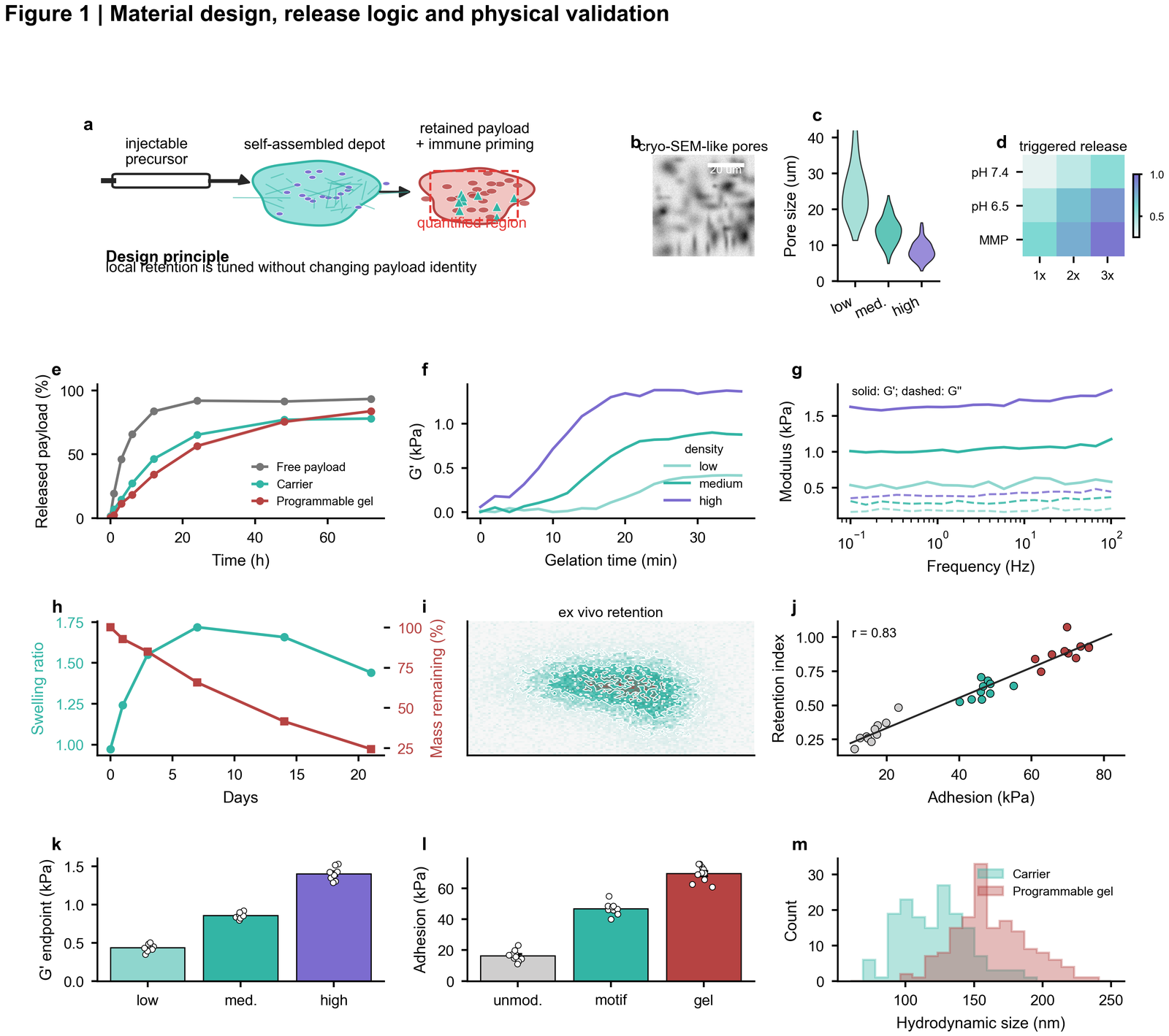 | Schematic-led composite, SEM-like image panel, rheology, release kinetics, retention map, correlation and endpoint quantification |
| Spatial retention and uptake |
| Schematic-led composite, SEM-like image panel, rheology, release kinetics, retention map, correlation and endpoint quantification |
| Spatial retention and uptake | 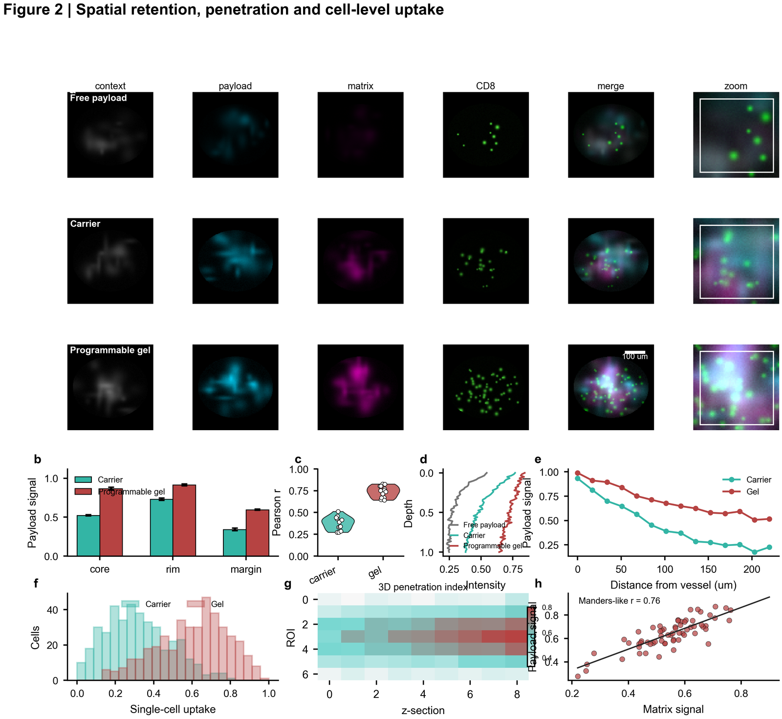 | Dark microscopy plate, channel rows, zoom crops, depth profiles, uptake histograms, 3D penetration heatmap and image-derived correlation |
| In vivo efficacy and tolerability |
| Dark microscopy plate, channel rows, zoom crops, depth profiles, uptake histograms, 3D penetration heatmap and image-derived correlation |
| In vivo efficacy and tolerability | 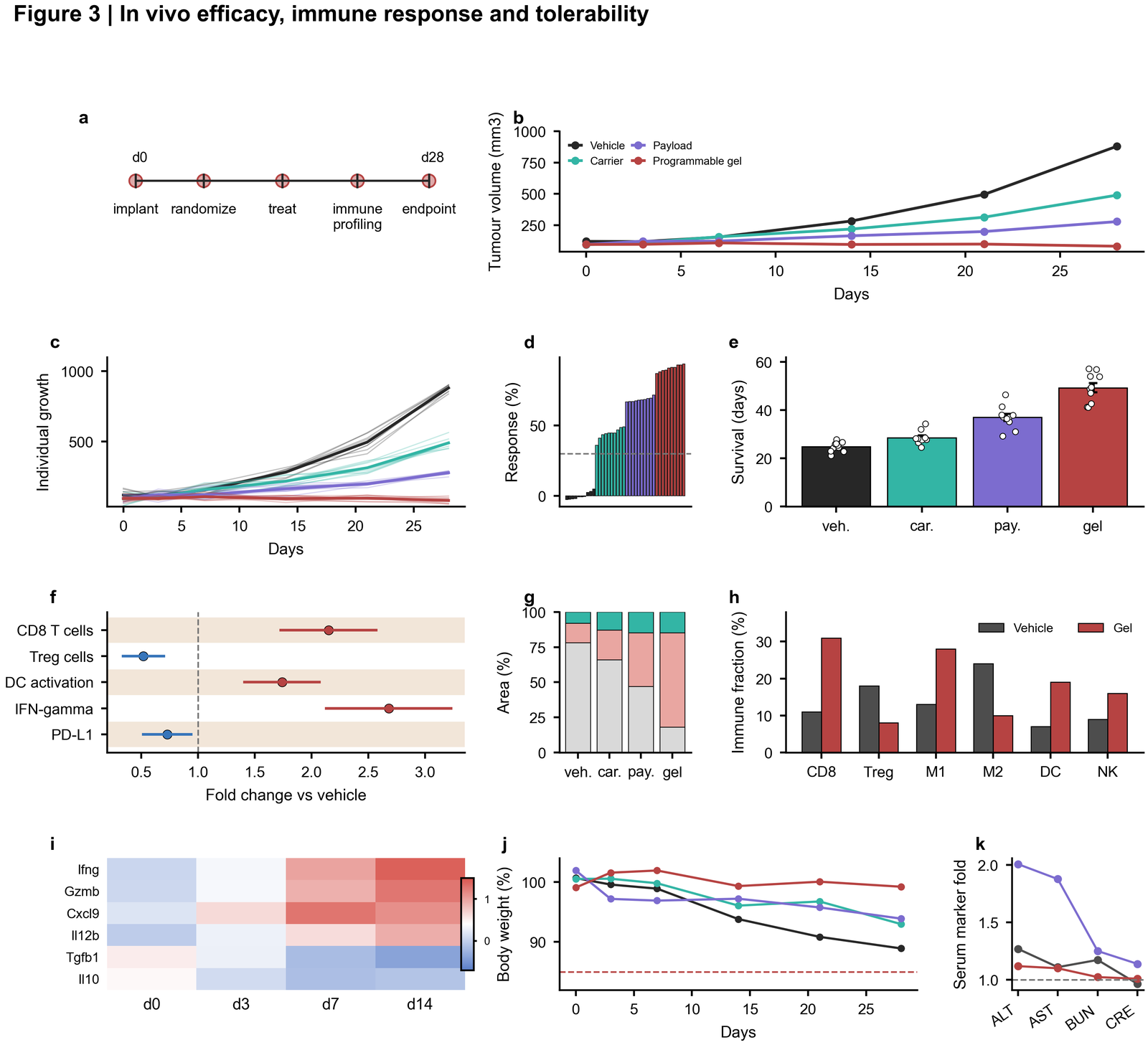 | Experimental timeline, longitudinal tumour curves, individual growth traces, waterfall response, forest plot, histology, immune composition and toxicity panels |
| Single-cell systems figure |
| Experimental timeline, longitudinal tumour curves, individual growth traces, waterfall response, forest plot, histology, immune composition and toxicity panels |
| Single-cell systems figure | 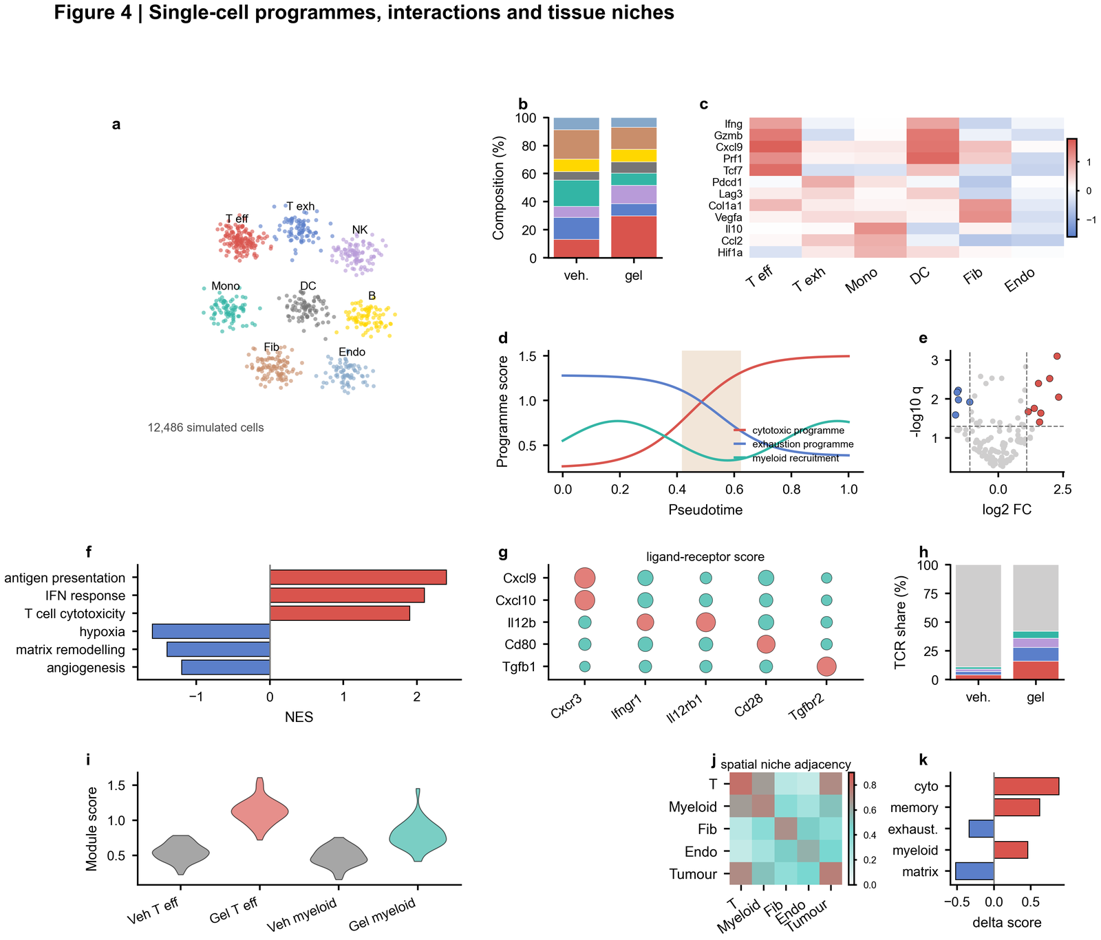 | UMAP-style embedding, composition, marker heatmap, pseudotime, volcano plot, enrichment, ligand-receptor bubble matrix and spatial niche adjacency |
| Perturbation validation |
| UMAP-style embedding, composition, marker heatmap, pseudotime, volcano plot, enrichment, ligand-receptor bubble matrix and spatial niche adjacency |
| Perturbation validation | 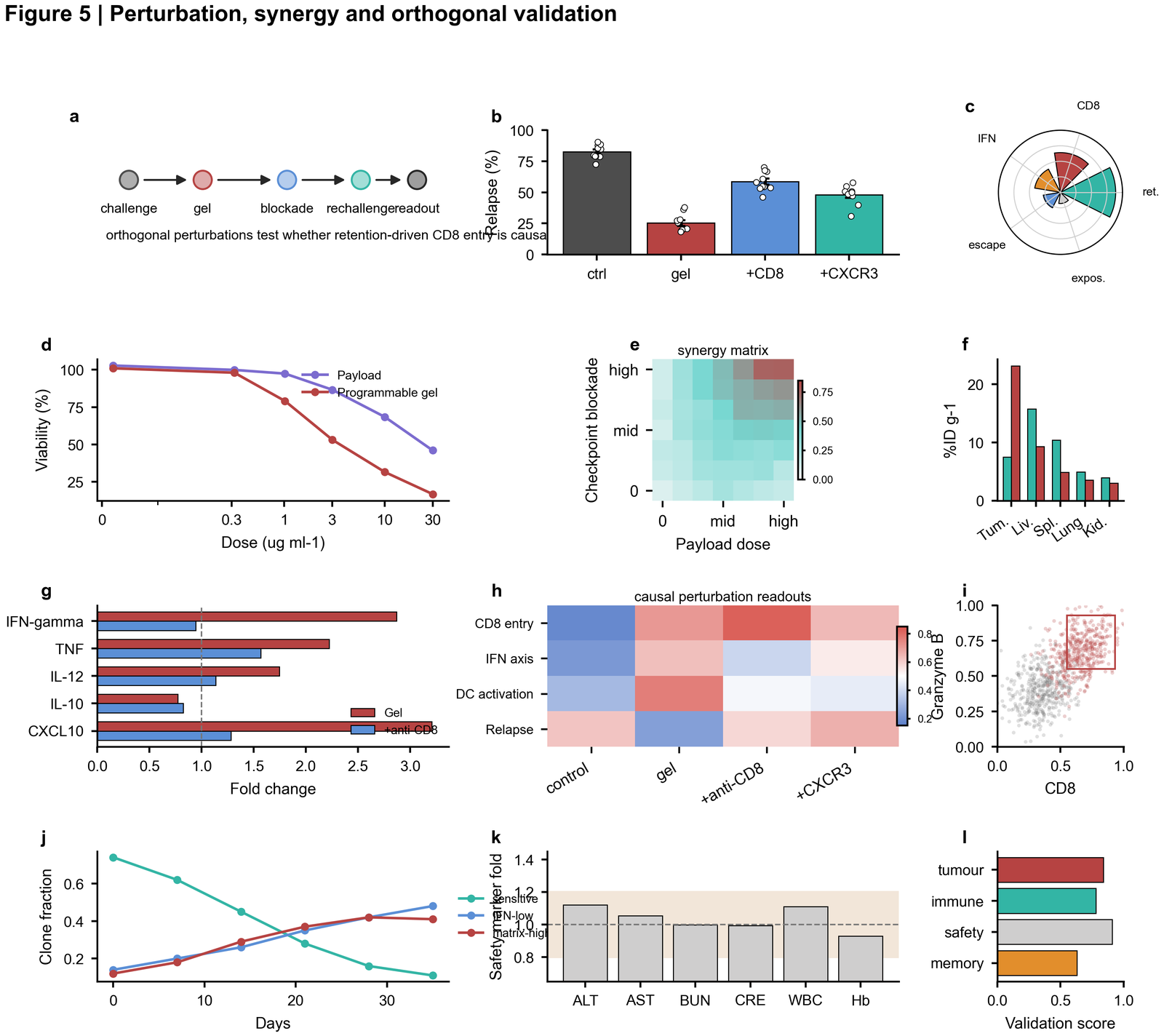 | Mechanistic perturbation timeline, relapse endpoint, polar summary, dose response, synergy matrix, biodistribution, cytokines, flow-like scatter and safety score |
**Gallery file policy**
Keep only lightweight PNG previews in `assets/gallery/`. Do not commit large generated
SVG/PDF outputs unless they are needed for a tutorial, because real users should regenerate
editable outputs from source data and scripts.
---
## Chart-type atlas
The gallery below classifies the skill by chart family. Each preview is a dense 4 x 4
atlas of small panels, designed to show the range of visual grammars that can be combined
inside a larger *Nature*-style result figure.
| Type | Preview | Common use |
|------|---------|------------|
| Bar charts |
| Mechanistic perturbation timeline, relapse endpoint, polar summary, dose response, synergy matrix, biodistribution, cytokines, flow-like scatter and safety score |
**Gallery file policy**
Keep only lightweight PNG previews in `assets/gallery/`. Do not commit large generated
SVG/PDF outputs unless they are needed for a tutorial, because real users should regenerate
editable outputs from source data and scripts.
---
## Chart-type atlas
The gallery below classifies the skill by chart family. Each preview is a dense 4 x 4
atlas of small panels, designed to show the range of visual grammars that can be combined
inside a larger *Nature*-style result figure.
| Type | Preview | Common use |
|------|---------|------------|
| Bar charts | 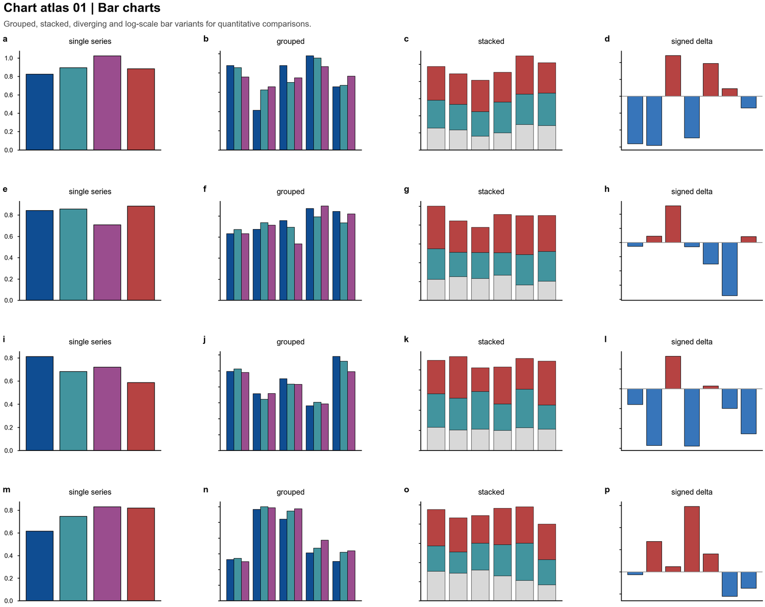 | Group comparisons, signed deltas, grouped-within-grouped designs, stacked composition |
| Line and longitudinal trends |
| Group comparisons, signed deltas, grouped-within-grouped designs, stacked composition |
| Line and longitudinal trends | 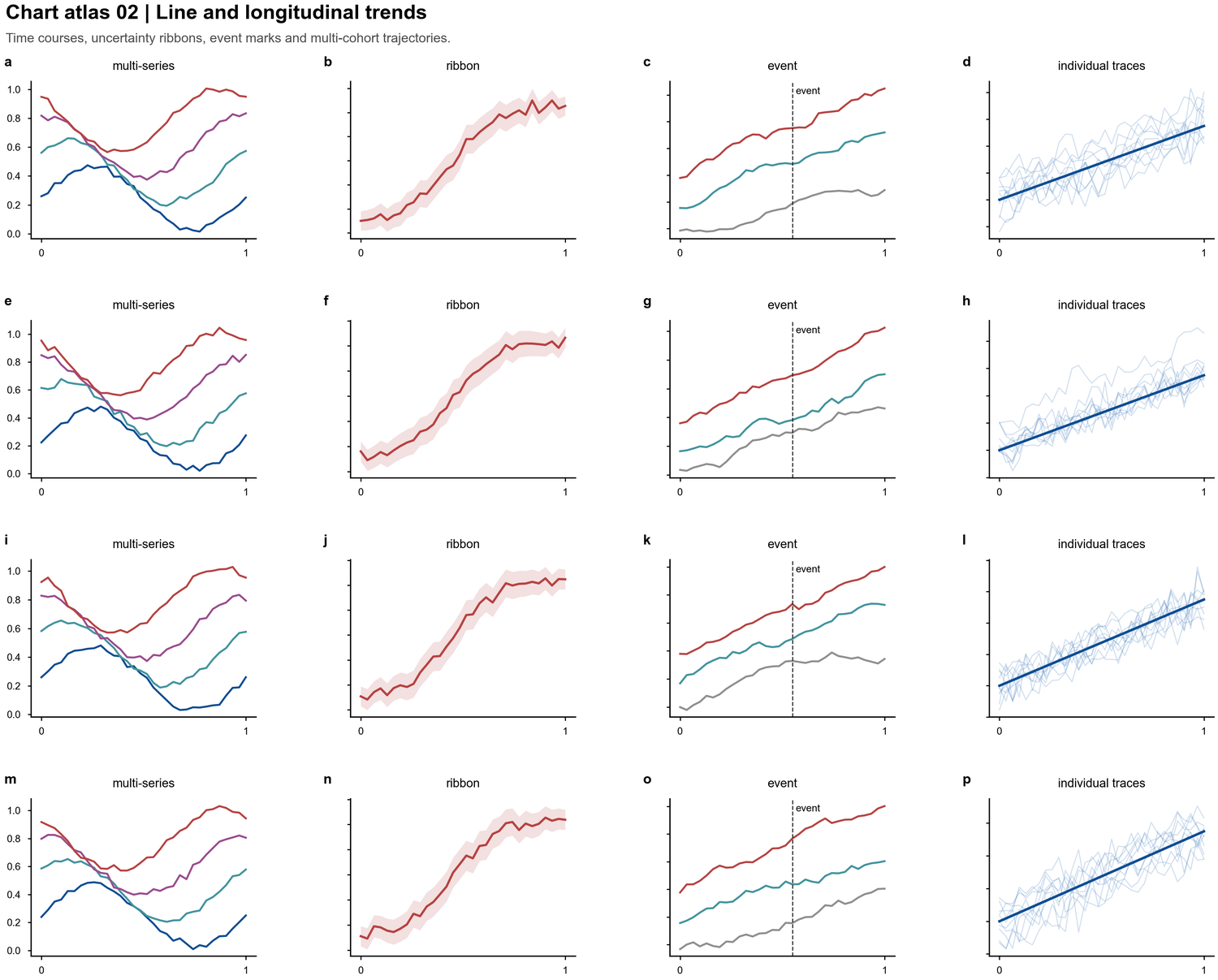 | Time courses, uncertainty ribbons, intervention marks, individual traces |
| Heatmaps |
| Time courses, uncertainty ribbons, intervention marks, individual traces |
| Heatmaps | 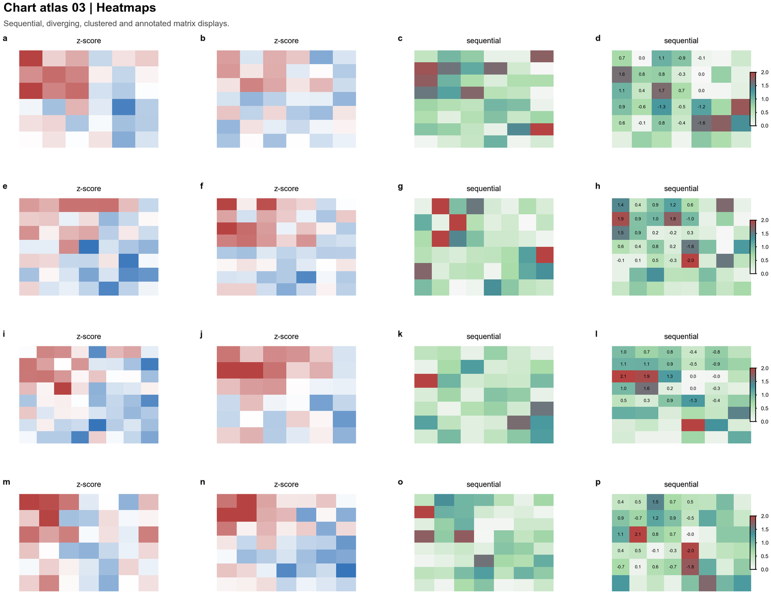 | Z-score matrices, sequential abundance maps, annotated tables, clustered blocks |
| Scatter and bubble plots |
| Z-score matrices, sequential abundance maps, annotated tables, clustered blocks |
| Scatter and bubble plots | 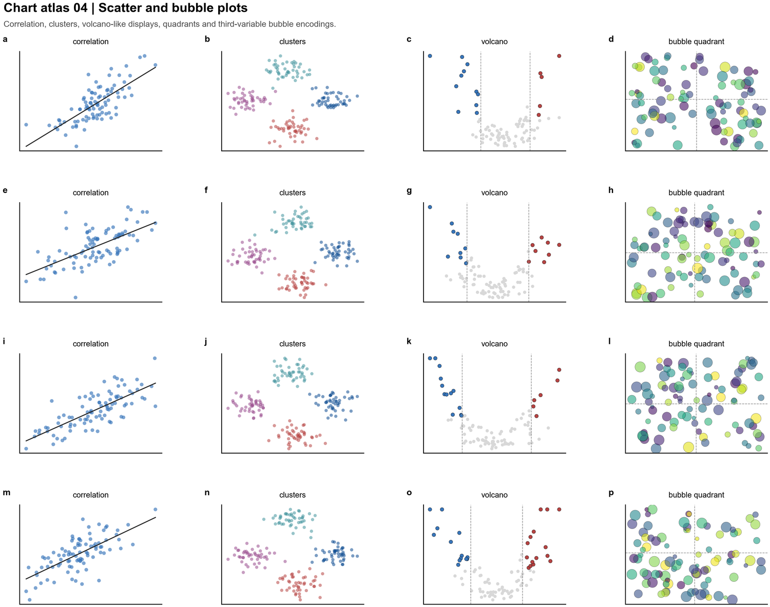 | Correlation, clusters, volcano-style tests, quadrant summaries, third-variable bubbles |
| Radar and polar charts |
| Correlation, clusters, volcano-style tests, quadrant summaries, third-variable bubbles |
| Radar and polar charts | 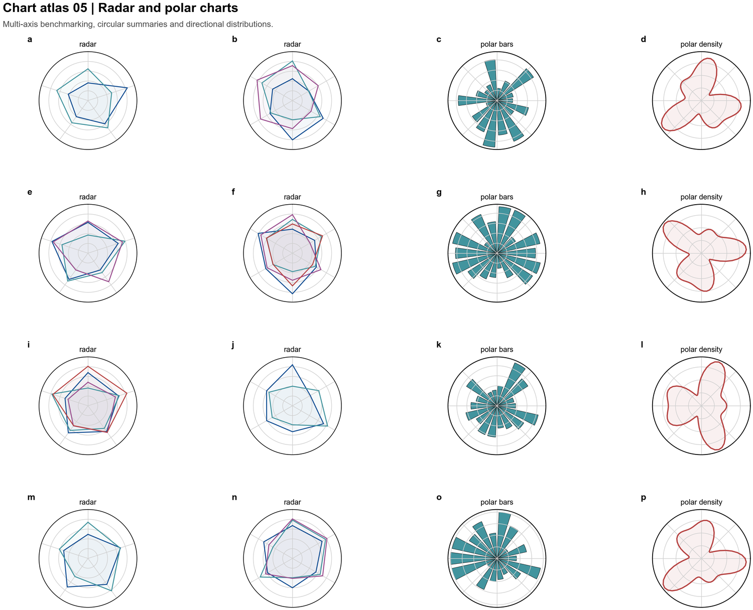 | Multi-axis benchmarking, circular summaries, polar histograms, directional density |
| Distribution plots |
| Multi-axis benchmarking, circular summaries, polar histograms, directional density |
| Distribution plots | 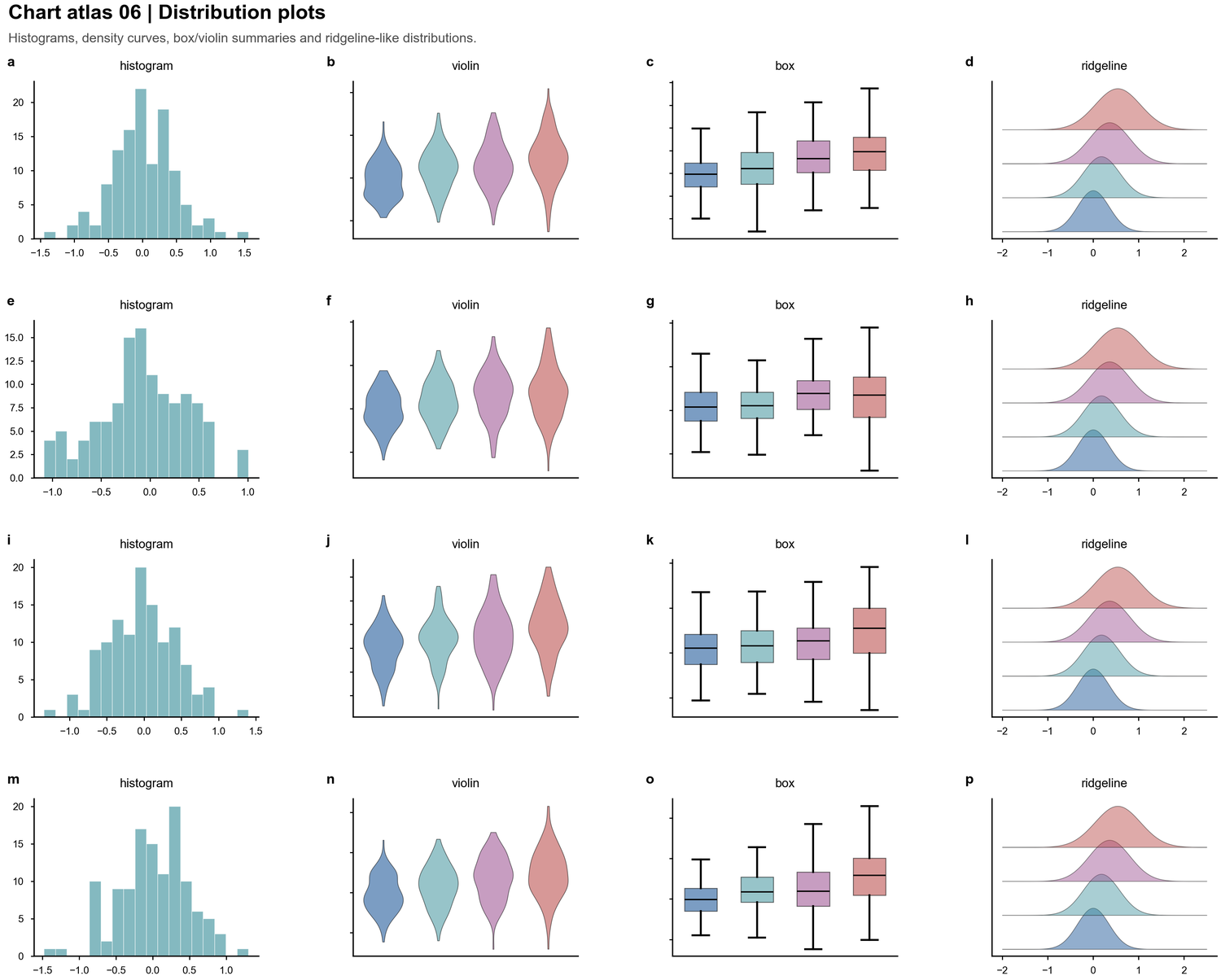 | Histograms, violins, boxes, ridgelines and sample-level spread |
| Forest and interval plots |
| Histograms, violins, boxes, ridgelines and sample-level spread |
| Forest and interval plots | 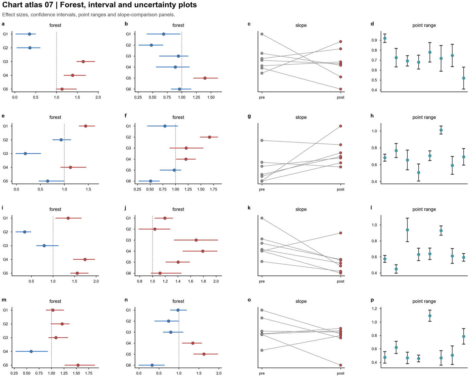 | Effect sizes, confidence intervals, point ranges, paired slope comparisons |
| Area and stacked trends |
| Effect sizes, confidence intervals, point ranges, paired slope comparisons |
| Area and stacked trends | 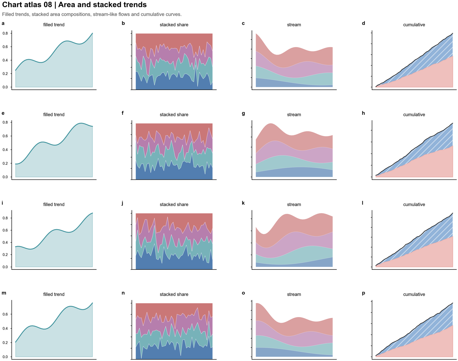 | Filled trajectories, stacked shares, cumulative curves, stream-like compositions |
| Image plates |
| Filled trajectories, stacked shares, cumulative curves, stream-like compositions |
| Image plates | 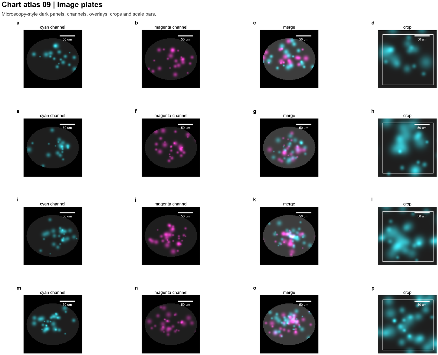 | Microscopy channels, overlays, crops, scale bars and dark-panel layouts |
| Network and matrix charts |
| Microscopy channels, overlays, crops, scale bars and dark-panel layouts |
| Network and matrix charts | 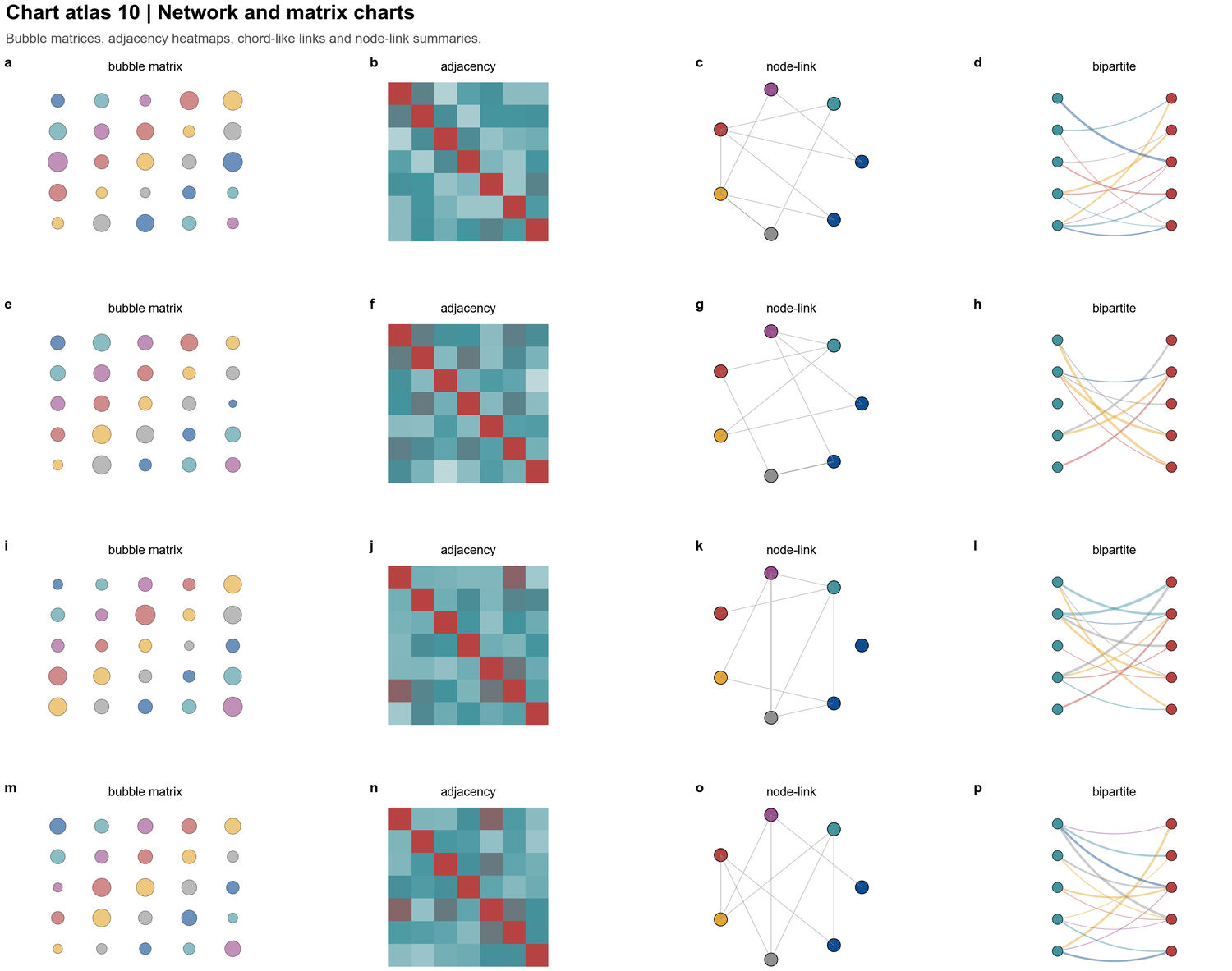 | Bubble matrices, adjacency maps, node-link diagrams and bipartite interaction panels |
---
## File structure
```
nature-figure/
├── SKILL.md ← skill trigger & overview (loaded by Claude automatically)
├── README.md ← this file
├── assets/
│ ├── gallery/ ← result-figure preview PNGs
│ └── chart-atlas/ ← chart-type taxonomy preview PNGs
└── references/
├── figure-contract.md ← core conclusion, evidence hierarchy, panel map
├── backend-selection.md ← Python vs R decision rules
├── r-workflow.md ← R scaffold, patchwork, ComplexHeatmap, export
├── r-template-index.md ← local R template atlas
├── qa-contract.md ← submission/revision QA checklist
├── api.md ← PALETTE constants, helper function signatures
├── design-theory.md ← typography, color theory, layout, export policy
├── common-patterns.md ← reusable code patterns (bars, legends, heatmaps)
├── tutorials.md ← end-to-end walkthroughs
└── chart-types.md ← radar, 3D sphere, scatter, fill_between, log-scale
```
---
## Backend and contract rules
Ask the user to choose **Python or R** unless the backend is already specified.
If they ask for a recommendation, use `references/backend-selection.md`.
After a backend is selected, use it exclusively for plotting, previews, exports,
and visual QA. If the selected runtime or packages are missing, stop and report the
blocker; do not render a fallback preview with the other language. This applies in
both directions: no Python substitute for R, and no R substitute for Python.
Before plotting, write or infer the core conclusion, figure archetype, panel map,
evidence hierarchy, target output, statistics/source-data needs, and export bundle.
The figure must serve the scientific logic first. Aesthetic polish and template
matching are secondary.
User-facing output must not disclose private local paths, private filenames, internal
reference documents, template identifiers, or private-material provenance unless the
user explicitly asks for that audit trail.
---
## Python mandatory rules
### 1. Three required rcParams — editable SVG text
```python
plt.rcParams['font.family'] = 'sans-serif'
plt.rcParams['font.sans-serif'] = ['Arial', 'DejaVu Sans', 'Liberation Sans']
plt.rcParams['svg.fonttype'] = 'none'
```
**Why `svg.fonttype = 'none'`**
Matplotlib's default (`'path'`) converts every glyph to a bezier curve. The result is
visually identical but every `` element becomes a `` — unselectable,
unsearchable, and impossible to realign in Illustrator or Inkscape.
With `'none'`, text stays as SVG `` nodes. Font substitution happens at render time.
**Why three fonts in the stack**
`Arial` is standard on macOS/Windows. `DejaVu Sans` ships with matplotlib and is the
Linux fallback. `Liberation Sans` is metric-compatible with Arial on RHEL/Ubuntu.
The cascade guarantees identical letter-spacing on all platforms.
### 2. Primary output format is SVG
```python
fig.savefig('figure.svg', bbox_inches='tight') # primary — editable text
fig.savefig('figure.png', dpi=300, bbox_inches='tight') # optional raster preview
```
Never use PNG alone when the figure will go into a paper or slide deck that requires
post-hoc text adjustment.
### 3. Always close the figure
```python
plt.close(fig)
```
---
## Quick-start template
```python
import matplotlib
matplotlib.use('Agg') # headless / server rendering
import matplotlib.pyplot as plt
import matplotlib.gridspec as gridspec
import numpy as np
# ── MANDATORY ─────────────────────────────────────────────────────────────────
plt.rcParams['font.family'] = 'sans-serif'
plt.rcParams['font.sans-serif'] = ['Arial', 'DejaVu Sans', 'Liberation Sans']
plt.rcParams['svg.fonttype'] = 'none'
# ── Style ──────────────────────────────────────────────────────────────────────
plt.rcParams.update({
'font.size': 12,
'axes.spines.right': False,
'axes.spines.top': False,
'axes.linewidth': 2.0,
'legend.frameon': False,
'xtick.major.width': 1.5,
'ytick.major.width': 1.5,
})
# ── Figure ──────────────────────────────────────────────────────────────────────
fig, ax = plt.subplots(figsize=(8, 5))
ax.spines['bottom'].set_linewidth(2)
ax.spines['left'].set_linewidth(2)
# ... your plot code ...
fig.tight_layout(pad=2)
fig.savefig('output.svg', bbox_inches='tight')
fig.savefig('output.png', dpi=300, bbox_inches='tight')
plt.close(fig)
```
---
## Color palette
```python
PALETTE = {
# Primary / hero method
'blue_main': '#0F4D92',
'blue_secondary': '#3775BA',
# Positive / improvement shades
'green_1': '#DDF3DE',
'green_2': '#AADCA9',
'green_3': '#8BCF8B',
# Baseline / contrast
'red_1': '#F6CFCB',
'red_2': '#E9A6A1',
'red_strong': '#B64342',
# Neutral support
'neutral_light': '#CFCECE',
'neutral_mid': '#767676',
'neutral_dark': '#4D4D4D',
'neutral_black': '#272727',
# Accent (use sparingly)
'gold': '#FFD700',
'teal': '#42949E',
'violet': '#9A4D8E',
'magenta': '#EA84DD',
}
```
**Semantic mapping convention**
`blue_main` = your method / hero series. `green_3` = positive variants. `red_strong` = baselines.
`neutral_light` = reference / background. Apply this consistently across every panel in the figure.
**Unified palette policy (recommended for recent Nature Machine Intelligence-style layouts)**
Do not maximize hue separation by default. In dense multi-panel figures, prefer **one coherent baseline family**
and **one coherent hero family**, then reserve green/red for delta markers or genuinely signed semantics.
```python
PALETTE_NMI_PASTEL = {
# Baseline / comparison family (cool blue-grey)
'baseline_dark': '#484878',
'baseline_mid': '#7884B4',
'baseline_soft': '#B4C0E4',
# Hero / proposed family (lilac → rose)
'ours_tiny': '#E4E4F0',
'ours_base': '#E4CCD8',
'ours_large': '#F0C0CC',
# Background blocks for overview / concept panels
'bg_lilac': '#E0E0F0',
'bg_aqua': '#E0F0F0',
'bg_peach': '#F0E0D0',
# Neutral support
'neutral_light': '#D8D8D8',
'neutral_mid': '#A8A8A8',
'neutral_dark': '#606060',
# Accent only for directional annotations
'delta_up': '#2E9E44',
'delta_down': '#E53935',
}
DEFAULT_COLORS_NMI_PASTEL = [
PALETTE_NMI_PASTEL['baseline_dark'],
PALETTE_NMI_PASTEL['baseline_mid'],
PALETTE_NMI_PASTEL['baseline_soft'],
PALETTE_NMI_PASTEL['ours_tiny'],
PALETTE_NMI_PASTEL['ours_base'],
PALETTE_NMI_PASTEL['ours_large'],
]
```
Use `DEFAULT_COLORS_NMI_PASTEL` when:
- comparing related model families such as `Tiny / Base / Large`
- building 1-page result atlases where multiple panels must feel visually unified
- matching low-saturation editorial styling rather than maximum category separation
**Practical rule**
The same method family keeps the same hue family in every panel. Do not recolor a model from blue-grey in panel `a`
to green in panel `d` just because that panel needs more contrast.
---
## Supported chart types
| Chart | File | Key pattern |
|-------|------|-------------|
| Grouped bar | `tutorials.md` | `ax.bar()` with `x + offset`, legend-only last panel |
| Stacked bar | `common-patterns.md` | iterate `col_order`, accumulate `bottom` |
| Horizontal ablation bar | `tutorials.md` | `ax.barh()`, alpha-gradient for completeness encoding |
| Trend / line | `tutorials.md` + `api.md` | `make_trend()`, `fill_between` for uncertainty shadow |
| Heatmap (sequential) | `api.md` | `make_heatmap()`, `YlOrRd`, cell annotation with luminance check |
| Heatmap (diverging / z-score) | `design-theory.md §11` | `RdBu_r`, `vmin=-2.5, vmax=2.5` |
| Bubble scatter | `design-theory.md §11` | x/y = two compartments, `s=` = third variable |
| Radar / polar | `chart-types.md` | `projection='polar'`, custom spokes, per-spoke normalization |
| 3D sphere / illustration | `chart-types.md` | Lambertian shading via ray-cast on numpy grid |
| Fill-between (stacked area) | `chart-types.md` | hatch for print-safe grayscale |
| Log-scale bar | `chart-types.md` | `set_yscale('log')`, expand top for annotations |
| Multi-panel GridSpec | `chart-types.md` | `GridSpec(rows, cols)`, `gs[0, :]` for full-width spans |
---
## Multi-panel information architecture
Each panel in a multi-panel figure must answer a **unique** scientific question.
Covering any one panel should leave a gap that cannot be recovered from the others.
### Three-level progressive complexity (recommended)
| Level | Question | Encoding |
|-------|----------|----------|
| Overview | "What is the landscape?" | Stacked bar, composition |
| Deviation | "What is distinctive per group?" | Z-score heatmap, diverging cmap |
| Relationship | "How do variables co-vary?" | Bubble scatter, correlation |
### Common redundancy traps
| Trap | Example | Fix |
|------|---------|-----|
| Absolute + absolute | Stacked bar (%) + heatmap of same % | Replace heatmap with z-score deviation |
| Subset of parent | Tumor-only ranked bar is just one column of the stacked bar | Swap for scatter: tumor % vs immune % |
| Two rankings | Two ranked bars on related metrics | Replace one with bubble scatter |
| Different chart, same data | Pie + stacked bar | Merge or replace with a relationship plot |
### Z-score deviation heatmap
```python
z = (heat - heat.mean(axis=0)) / heat.std(axis=0)
im = ax.imshow(z.values, cmap='RdBu_r', aspect='auto', vmin=-2.5, vmax=2.5)
cbar.set_label('Z-score vs pan-cohort mean')
```
`RdBu_r`: red = enriched above average, blue = depleted. Orthogonal to absolute % shown in panel a.
### Bubble scatter with quadrant labels
```python
ax.scatter(x, y, s=size_var * scale, c=colors, edgecolors='white', linewidth=0.8, alpha=0.9)
ax.axvline(np.median(x), lw=1.2, ls='--', color='#767676', alpha=0.6)
ax.axhline(np.median(y), lw=1.2, ls='--', color='#767676', alpha=0.6)
```
Label quadrants at corners with small grey italic text (`fontsize=7.5, color='#888888', style='italic'`).
---
## Layout rules
### Figure sizes
| Type | `figsize` |
|------|-----------|
| Multi-metric bar (3–4 metrics + legend panel) | `(28–45, 6–12)` |
| Grand multi-panel (3 panels, 2-row GridSpec) | `(22, 17)` |
| Compact single bar | `(9–16, 5–8)` |
| Trend / line multi-panel | `(14, 4)` or `(9, 8)` |
| Heatmap single | `(8–20, 5–9)` |
| Radar polar | `(12, 10)` |
**Rule**: width ≈ 3–4× height for comparison bar panels.
### Panel labels
```python
ax.text(-0.05, 1.06, 'a', transform=ax.transAxes,
fontsize=22, fontweight='bold', va='top', ha='right')
```
Use lowercase bold (`a`, `b`, `c`) at top-left of each subplot axes, placed via `transAxes`.
### Legend
- For multi-axis figures: give the legend its own axis (`ax.set_axis_off()`).
- Always `frameon=False`.
- When the legend is large, place it `bbox_to_anchor=(0.5, -0.24), loc='upper center'` below the panel.
---
## Font size hierarchy
| Context | `font.size` |
|---------|-------------|
| Base (compact subfigures) | 12–16 |
| Large bar panels (figsize > 28 in) | 24 |
| Axis labels (large panels) | 32–54 via per-label override |
| In-bar / in-cell annotations | 6.5–12 |
| Panel letter labels | 20–22 |
| Legend | 8–14 |
---
## Axes & spines rules
```python
plt.rcParams['axes.spines.right'] = False # always off
plt.rcParams['axes.spines.top'] = False # always off
plt.rcParams['legend.frameon'] = False
ax.spines['bottom'].set_linewidth(2) # thicker for emphasis
ax.spines['left'].set_linewidth(2)
```
No gridlines by default. Use sparse `set_yticks` to guide the eye.
Y-limits tightened to data range — never use `0–100` when all values sit in `80–95`.
---
## In-cell / in-bar text contrast
```python
def luminance_text_color(hex_color):
c = hex_color.lstrip('#')
r, g, b = int(c[0:2],16)/255, int(c[2:4],16)/255, int(c[4:6],16)/255
return 'white' if 0.299*r + 0.587*g + 0.114*b < 0.5 else '#333333'
```
---
## Reproduction checklist
- [ ] Core conclusion and panel map are clear before styling
- [ ] Backend is explicitly Python or R
- [ ] **Lines 1–3**: `font.family`, `font.sans-serif` (three fonts), `svg.fonttype = 'none'`
- [ ] Primary output is **SVG** (`bbox_inches='tight'`)
- [ ] Right and top spines off; `legend.frameon = False`
- [ ] Font size matches final use: 5–7 pt for dense journal output, larger only for slide-sized panels
- [ ] Colors come from one coherent palette system: either semantic `PALETTE` or unified `PALETTE_NMI_PASTEL`
- [ ] Related model sizes / variants share a hue family; do not assign unrelated saturated colors to siblings
- [ ] Green / red reserved for gains, drops, thresholds, or truly signed semantics
- [ ] Y-limits tightened to data range
- [ ] Multi-panel figures: each panel answers a **different** question (anti-redundancy checklist passed)
- [ ] Panel labels (`a`, `b`, `c`) are bold lowercase and sized for final output
- [ ] Statistics, `n`, source data, and image-integrity notes are documented when manuscript-facing
- [ ] `tight_layout(pad=2)` before save
- [ ] `plt.close(fig)` after save
| Bubble matrices, adjacency maps, node-link diagrams and bipartite interaction panels |
---
## File structure
```
nature-figure/
├── SKILL.md ← skill trigger & overview (loaded by Claude automatically)
├── README.md ← this file
├── assets/
│ ├── gallery/ ← result-figure preview PNGs
│ └── chart-atlas/ ← chart-type taxonomy preview PNGs
└── references/
├── figure-contract.md ← core conclusion, evidence hierarchy, panel map
├── backend-selection.md ← Python vs R decision rules
├── r-workflow.md ← R scaffold, patchwork, ComplexHeatmap, export
├── r-template-index.md ← local R template atlas
├── qa-contract.md ← submission/revision QA checklist
├── api.md ← PALETTE constants, helper function signatures
├── design-theory.md ← typography, color theory, layout, export policy
├── common-patterns.md ← reusable code patterns (bars, legends, heatmaps)
├── tutorials.md ← end-to-end walkthroughs
└── chart-types.md ← radar, 3D sphere, scatter, fill_between, log-scale
```
---
## Backend and contract rules
Ask the user to choose **Python or R** unless the backend is already specified.
If they ask for a recommendation, use `references/backend-selection.md`.
After a backend is selected, use it exclusively for plotting, previews, exports,
and visual QA. If the selected runtime or packages are missing, stop and report the
blocker; do not render a fallback preview with the other language. This applies in
both directions: no Python substitute for R, and no R substitute for Python.
Before plotting, write or infer the core conclusion, figure archetype, panel map,
evidence hierarchy, target output, statistics/source-data needs, and export bundle.
The figure must serve the scientific logic first. Aesthetic polish and template
matching are secondary.
User-facing output must not disclose private local paths, private filenames, internal
reference documents, template identifiers, or private-material provenance unless the
user explicitly asks for that audit trail.
---
## Python mandatory rules
### 1. Three required rcParams — editable SVG text
```python
plt.rcParams['font.family'] = 'sans-serif'
plt.rcParams['font.sans-serif'] = ['Arial', 'DejaVu Sans', 'Liberation Sans']
plt.rcParams['svg.fonttype'] = 'none'
```
**Why `svg.fonttype = 'none'`**
Matplotlib's default (`'path'`) converts every glyph to a bezier curve. The result is
visually identical but every `` element becomes a `` — unselectable,
unsearchable, and impossible to realign in Illustrator or Inkscape.
With `'none'`, text stays as SVG `` nodes. Font substitution happens at render time.
**Why three fonts in the stack**
`Arial` is standard on macOS/Windows. `DejaVu Sans` ships with matplotlib and is the
Linux fallback. `Liberation Sans` is metric-compatible with Arial on RHEL/Ubuntu.
The cascade guarantees identical letter-spacing on all platforms.
### 2. Primary output format is SVG
```python
fig.savefig('figure.svg', bbox_inches='tight') # primary — editable text
fig.savefig('figure.png', dpi=300, bbox_inches='tight') # optional raster preview
```
Never use PNG alone when the figure will go into a paper or slide deck that requires
post-hoc text adjustment.
### 3. Always close the figure
```python
plt.close(fig)
```
---
## Quick-start template
```python
import matplotlib
matplotlib.use('Agg') # headless / server rendering
import matplotlib.pyplot as plt
import matplotlib.gridspec as gridspec
import numpy as np
# ── MANDATORY ─────────────────────────────────────────────────────────────────
plt.rcParams['font.family'] = 'sans-serif'
plt.rcParams['font.sans-serif'] = ['Arial', 'DejaVu Sans', 'Liberation Sans']
plt.rcParams['svg.fonttype'] = 'none'
# ── Style ──────────────────────────────────────────────────────────────────────
plt.rcParams.update({
'font.size': 12,
'axes.spines.right': False,
'axes.spines.top': False,
'axes.linewidth': 2.0,
'legend.frameon': False,
'xtick.major.width': 1.5,
'ytick.major.width': 1.5,
})
# ── Figure ──────────────────────────────────────────────────────────────────────
fig, ax = plt.subplots(figsize=(8, 5))
ax.spines['bottom'].set_linewidth(2)
ax.spines['left'].set_linewidth(2)
# ... your plot code ...
fig.tight_layout(pad=2)
fig.savefig('output.svg', bbox_inches='tight')
fig.savefig('output.png', dpi=300, bbox_inches='tight')
plt.close(fig)
```
---
## Color palette
```python
PALETTE = {
# Primary / hero method
'blue_main': '#0F4D92',
'blue_secondary': '#3775BA',
# Positive / improvement shades
'green_1': '#DDF3DE',
'green_2': '#AADCA9',
'green_3': '#8BCF8B',
# Baseline / contrast
'red_1': '#F6CFCB',
'red_2': '#E9A6A1',
'red_strong': '#B64342',
# Neutral support
'neutral_light': '#CFCECE',
'neutral_mid': '#767676',
'neutral_dark': '#4D4D4D',
'neutral_black': '#272727',
# Accent (use sparingly)
'gold': '#FFD700',
'teal': '#42949E',
'violet': '#9A4D8E',
'magenta': '#EA84DD',
}
```
**Semantic mapping convention**
`blue_main` = your method / hero series. `green_3` = positive variants. `red_strong` = baselines.
`neutral_light` = reference / background. Apply this consistently across every panel in the figure.
**Unified palette policy (recommended for recent Nature Machine Intelligence-style layouts)**
Do not maximize hue separation by default. In dense multi-panel figures, prefer **one coherent baseline family**
and **one coherent hero family**, then reserve green/red for delta markers or genuinely signed semantics.
```python
PALETTE_NMI_PASTEL = {
# Baseline / comparison family (cool blue-grey)
'baseline_dark': '#484878',
'baseline_mid': '#7884B4',
'baseline_soft': '#B4C0E4',
# Hero / proposed family (lilac → rose)
'ours_tiny': '#E4E4F0',
'ours_base': '#E4CCD8',
'ours_large': '#F0C0CC',
# Background blocks for overview / concept panels
'bg_lilac': '#E0E0F0',
'bg_aqua': '#E0F0F0',
'bg_peach': '#F0E0D0',
# Neutral support
'neutral_light': '#D8D8D8',
'neutral_mid': '#A8A8A8',
'neutral_dark': '#606060',
# Accent only for directional annotations
'delta_up': '#2E9E44',
'delta_down': '#E53935',
}
DEFAULT_COLORS_NMI_PASTEL = [
PALETTE_NMI_PASTEL['baseline_dark'],
PALETTE_NMI_PASTEL['baseline_mid'],
PALETTE_NMI_PASTEL['baseline_soft'],
PALETTE_NMI_PASTEL['ours_tiny'],
PALETTE_NMI_PASTEL['ours_base'],
PALETTE_NMI_PASTEL['ours_large'],
]
```
Use `DEFAULT_COLORS_NMI_PASTEL` when:
- comparing related model families such as `Tiny / Base / Large`
- building 1-page result atlases where multiple panels must feel visually unified
- matching low-saturation editorial styling rather than maximum category separation
**Practical rule**
The same method family keeps the same hue family in every panel. Do not recolor a model from blue-grey in panel `a`
to green in panel `d` just because that panel needs more contrast.
---
## Supported chart types
| Chart | File | Key pattern |
|-------|------|-------------|
| Grouped bar | `tutorials.md` | `ax.bar()` with `x + offset`, legend-only last panel |
| Stacked bar | `common-patterns.md` | iterate `col_order`, accumulate `bottom` |
| Horizontal ablation bar | `tutorials.md` | `ax.barh()`, alpha-gradient for completeness encoding |
| Trend / line | `tutorials.md` + `api.md` | `make_trend()`, `fill_between` for uncertainty shadow |
| Heatmap (sequential) | `api.md` | `make_heatmap()`, `YlOrRd`, cell annotation with luminance check |
| Heatmap (diverging / z-score) | `design-theory.md §11` | `RdBu_r`, `vmin=-2.5, vmax=2.5` |
| Bubble scatter | `design-theory.md §11` | x/y = two compartments, `s=` = third variable |
| Radar / polar | `chart-types.md` | `projection='polar'`, custom spokes, per-spoke normalization |
| 3D sphere / illustration | `chart-types.md` | Lambertian shading via ray-cast on numpy grid |
| Fill-between (stacked area) | `chart-types.md` | hatch for print-safe grayscale |
| Log-scale bar | `chart-types.md` | `set_yscale('log')`, expand top for annotations |
| Multi-panel GridSpec | `chart-types.md` | `GridSpec(rows, cols)`, `gs[0, :]` for full-width spans |
---
## Multi-panel information architecture
Each panel in a multi-panel figure must answer a **unique** scientific question.
Covering any one panel should leave a gap that cannot be recovered from the others.
### Three-level progressive complexity (recommended)
| Level | Question | Encoding |
|-------|----------|----------|
| Overview | "What is the landscape?" | Stacked bar, composition |
| Deviation | "What is distinctive per group?" | Z-score heatmap, diverging cmap |
| Relationship | "How do variables co-vary?" | Bubble scatter, correlation |
### Common redundancy traps
| Trap | Example | Fix |
|------|---------|-----|
| Absolute + absolute | Stacked bar (%) + heatmap of same % | Replace heatmap with z-score deviation |
| Subset of parent | Tumor-only ranked bar is just one column of the stacked bar | Swap for scatter: tumor % vs immune % |
| Two rankings | Two ranked bars on related metrics | Replace one with bubble scatter |
| Different chart, same data | Pie + stacked bar | Merge or replace with a relationship plot |
### Z-score deviation heatmap
```python
z = (heat - heat.mean(axis=0)) / heat.std(axis=0)
im = ax.imshow(z.values, cmap='RdBu_r', aspect='auto', vmin=-2.5, vmax=2.5)
cbar.set_label('Z-score vs pan-cohort mean')
```
`RdBu_r`: red = enriched above average, blue = depleted. Orthogonal to absolute % shown in panel a.
### Bubble scatter with quadrant labels
```python
ax.scatter(x, y, s=size_var * scale, c=colors, edgecolors='white', linewidth=0.8, alpha=0.9)
ax.axvline(np.median(x), lw=1.2, ls='--', color='#767676', alpha=0.6)
ax.axhline(np.median(y), lw=1.2, ls='--', color='#767676', alpha=0.6)
```
Label quadrants at corners with small grey italic text (`fontsize=7.5, color='#888888', style='italic'`).
---
## Layout rules
### Figure sizes
| Type | `figsize` |
|------|-----------|
| Multi-metric bar (3–4 metrics + legend panel) | `(28–45, 6–12)` |
| Grand multi-panel (3 panels, 2-row GridSpec) | `(22, 17)` |
| Compact single bar | `(9–16, 5–8)` |
| Trend / line multi-panel | `(14, 4)` or `(9, 8)` |
| Heatmap single | `(8–20, 5–9)` |
| Radar polar | `(12, 10)` |
**Rule**: width ≈ 3–4× height for comparison bar panels.
### Panel labels
```python
ax.text(-0.05, 1.06, 'a', transform=ax.transAxes,
fontsize=22, fontweight='bold', va='top', ha='right')
```
Use lowercase bold (`a`, `b`, `c`) at top-left of each subplot axes, placed via `transAxes`.
### Legend
- For multi-axis figures: give the legend its own axis (`ax.set_axis_off()`).
- Always `frameon=False`.
- When the legend is large, place it `bbox_to_anchor=(0.5, -0.24), loc='upper center'` below the panel.
---
## Font size hierarchy
| Context | `font.size` |
|---------|-------------|
| Base (compact subfigures) | 12–16 |
| Large bar panels (figsize > 28 in) | 24 |
| Axis labels (large panels) | 32–54 via per-label override |
| In-bar / in-cell annotations | 6.5–12 |
| Panel letter labels | 20–22 |
| Legend | 8–14 |
---
## Axes & spines rules
```python
plt.rcParams['axes.spines.right'] = False # always off
plt.rcParams['axes.spines.top'] = False # always off
plt.rcParams['legend.frameon'] = False
ax.spines['bottom'].set_linewidth(2) # thicker for emphasis
ax.spines['left'].set_linewidth(2)
```
No gridlines by default. Use sparse `set_yticks` to guide the eye.
Y-limits tightened to data range — never use `0–100` when all values sit in `80–95`.
---
## In-cell / in-bar text contrast
```python
def luminance_text_color(hex_color):
c = hex_color.lstrip('#')
r, g, b = int(c[0:2],16)/255, int(c[2:4],16)/255, int(c[4:6],16)/255
return 'white' if 0.299*r + 0.587*g + 0.114*b < 0.5 else '#333333'
```
---
## Reproduction checklist
- [ ] Core conclusion and panel map are clear before styling
- [ ] Backend is explicitly Python or R
- [ ] **Lines 1–3**: `font.family`, `font.sans-serif` (three fonts), `svg.fonttype = 'none'`
- [ ] Primary output is **SVG** (`bbox_inches='tight'`)
- [ ] Right and top spines off; `legend.frameon = False`
- [ ] Font size matches final use: 5–7 pt for dense journal output, larger only for slide-sized panels
- [ ] Colors come from one coherent palette system: either semantic `PALETTE` or unified `PALETTE_NMI_PASTEL`
- [ ] Related model sizes / variants share a hue family; do not assign unrelated saturated colors to siblings
- [ ] Green / red reserved for gains, drops, thresholds, or truly signed semantics
- [ ] Y-limits tightened to data range
- [ ] Multi-panel figures: each panel answers a **different** question (anti-redundancy checklist passed)
- [ ] Panel labels (`a`, `b`, `c`) are bold lowercase and sized for final output
- [ ] Statistics, `n`, source data, and image-integrity notes are documented when manuscript-facing
- [ ] `tight_layout(pad=2)` before save
- [ ] `plt.close(fig)` after save