{
"cells": [
{
"cell_type": "markdown",
"metadata": {},
"source": [
"## State-feedback Stabilization"
]
},
{
"cell_type": "markdown",
"metadata": {},
"source": [
"Consider a linear ordinary differential equation (ODE), given by\n",
"\n",
"$$\\frac{{\\rm{d}}}{{\\rm{d}}t}x = A x, \\quad x\\in \\mathbb{R}^{n}, \\quad A\\in \\mathbb{R}^{n\\times n}.$$\n",
"\n",
"It is well-known that if any of the $n$ eigenvalues of $A$ has positive real part, then the above ODE is unstable, i.e., starting from any initial condition $x(0)$, the ODE solution trajectory $x(t) \\rightarrow \\infty$ as $t\\rightarrow\\infty$. In practical applications, the components of vector $x$ has physical meaning, such as position and velocity, which going to infinity implies system failure (e.g., crash/explosion/other bad things). However, many physical systems do have such unstable $A$ matrix. One basic problem in control theory is to modify the above ODE as\n",
"\n",
"$$\\frac{{\\rm{d}}}{{\\rm{d}}t}x = A x \\:+\\: Bu, \\quad u\\in \\mathbb{R}^{m}, \\quad B\\in \\mathbb{R}^{n\\times m},$$\n",
"\n",
"where the function $u(x)$ needs to be designed in such a way that starting from any initial condition $x(0)$, the trajectory $x(t) \\rightarrow 0$ as $t \\rightarrow \\infty$, i.e., the system becomes globally asymptotically stable. The quantity $x\\in\\mathbb{R}^{n}$ is called the \"state\", and $u\\in\\mathbb{R}^{m}$ is called the \"control\". The matrix $B$ reflects control authority, i.e., our ability to manipulate the states. The function $u(x)$ is called state-feedback. In this exercise, we consider linear (static) state-feedback stabilization problem, i.e., to design a constant matrix $K\\in\\mathbb{R}^{m\\times n}$ such that $u(x)=Kx$ stabilizes the ODE."
]
},
{
"cell_type": "markdown",
"metadata": {},
"source": [
"(a) **[15 points]** With the above choice of $u(x)$, our ODE becomes $\\frac{{\\rm{d}}}{{\\rm{d}}t}x = (A + BK)x$, which is still a linear ODE. A fundamental theorem in control theory says that a linear ODE is globally asymptotically stable if and only if there exists a function $V(x) = x^{\\top}Px$ such that for all $x\\neq 0$, the function $V(x)$ is strictly positive, and $\\frac{{\\rm{d}}}{{\\rm{d}}t}V < 0.$ Prove that designing the matrix $K$ is equivalent to solving two coupled inequalities in matrix variable pair $(P,K)$, given by\n",
"\n",
"$$P \\succ 0, \\qquad PA + A^{\\top}P + PBK + K^{\\top}B^{\\top}P \\prec 0.$$"
]
},
{
"cell_type": "markdown",
"metadata": {},
"source": [
"#### Solution:\n",
"The function $V(x) = x^{\\top}Px > 0$ for all $x\\neq 0$ if and only if $P \\succ 0$. Furthermore, the condition $\\frac{{\\rm{d}}}{{\\rm{d}}t}V < 0$ is equivalent to\n",
"\n",
"$$\\frac{{\\rm{d}}}{{\\rm{d}}t}V = \\left(\\frac{{\\rm{d}}x}{{\\rm{d}}t}\\right)^{\\top}P x \\:+\\: x^{\\top}P\\frac{{\\rm{d}}x}{{\\rm{d}}t} = x^{\\top}\\left(\\left(A^{\\top}+K^{\\top}B^{\\top}\\right)P \\: + \\: P\\left(A+BK\\right)\\right)x < 0, \\quad \\text{for all}\\quad x,$$\n",
"\n",
"i.e., $PA + A^{\\top}P + PBK + K^{\\top}B^{\\top}P \\prec 0$. Hence the statement. "
]
},
{
"cell_type": "markdown",
"metadata": {},
"source": [
"(b) **[5 points]** Are the two matrix inequalities derived in part (a) LMIs? Why/why not?"
]
},
{
"cell_type": "markdown",
"metadata": {},
"source": [
"#### Solution:\n",
"The inequality $P \\succ 0$ is an LMI. However, the inequality $PA + A^{\\top}P + PBK + K^{\\top}B^{\\top}P \\prec 0$ is **not an LMI** due to the last two summands, which are bilinear in $P$ and $K$, and hence called a \"bilinear matrix inequality\" (BMI)."
]
},
{
"cell_type": "markdown",
"metadata": {},
"source": [
"(c) **[20 points]** Introduce the change-of-variables $(P,K) \\mapsto (Q,L)$, given by $Q = P^{-1}$, $L=KP^{-1}$, to rewrite the matrix inequalities derived in part (a) as LMIs in new matrix variables $(Q,L)$."
]
},
{
"cell_type": "markdown",
"metadata": {},
"source": [
"#### Solution:\n",
"Since matrix inversion preserves positive definiteness, hence $P \\succ 0 \\: \\Leftrightarrow \\: Q \\succ 0$. On the other hand,\n",
"\n",
"$$PA + A^{\\top}P + PBK + K^{\\top}B^{\\top}P \\prec 0 \\: \\Leftrightarrow \\: Q^{-1}A + A^{\\top}Q^{-1} + Q^{-1}BLQ^{-1} + Q^{-1}L^{\\top}B^{\\top}Q^{-1} \\prec 0.$$\n",
"\n",
"Since congruence transformation by invertible matrix $Q$ (i.e., left and right multiplying the LHS by $Q$) applied to the LHS of the last inequality should preserve sign-definiteness, hence we get\n",
"\n",
"$$AQ + QA^{\\top} + BL + L^{\\top}B^{\\top} \\prec 0,$$\n",
"\n",
"which is an LMI. Thus, our LMIs are $Q \\succ 0$, $AQ + QA^{\\top} + BL + L^{\\top}B^{\\top} \\prec 0$."
]
},
{
"cell_type": "markdown",
"metadata": {},
"source": [
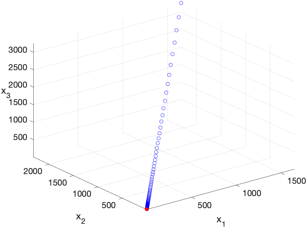
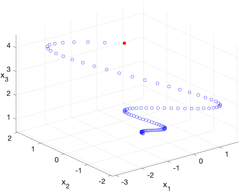
"(d) **[10 points]** Since the inequalities that you derive in part (c) are LMIs, we can ask cvx/cvxpy to solve that convex feasibility problem, i.e., to find a feasible pair $(Q,L)$ satisfying those LMIs. This is same as saying we can use cvx/cvxpy to design a mathematically provable globally stabilizing controller, i.e., to compute $K$. \n",
"\n",
"As an example system in $\\mathbb{R}^{3}$, the following left plot shows the uncontrolled trajectory $x(t)$, with $A = \\begin{pmatrix}\n",
"-0.5 & 0.3 & 0.4\\\\\n",
"1 & 0 & 0\\\\\n",
"0 & 1 & 0\\end{pmatrix}$, $t\\in[0,5]$, and initial condition $x(0)=(1,2,3)^{\\top}$ (red solid point). The following right plot shows the controlled trajectory for the same data, where the state-feedback controller $u(x)=Kx$ is derived using cvx with $B = (1,0,0)^{\\top}$. This shows that the system is unstable (without feedback) but state-feedback stabilizable."
]
},
{
"cell_type": "markdown",
"metadata": {},
"source": [
""
]
},
{
"cell_type": "markdown",
"metadata": {},
"source": [
"We can do more. If we want the rate of convergence to be faster than $\\exp\\left(-\\alpha t\\right)$, where $\\alpha > 0$ is some given parameter, then the condition $\\frac{{\\rm{d}}}{{\\rm{d}}t}V < 0$ needs to be replaced by $\\frac{{\\rm{d}}}{{\\rm{d}}t}V < -\\alpha V$. Modify your LMIs from part (c) to derive a new set of LMIs guaranteeing this condition (hence the controller can again be derived via cvx/cvxpy). As an example, the following plot shows the controlled trajectory with previous data and $\\alpha=2$."
]
},
{
"cell_type": "markdown",
"metadata": {},
"source": [
" "
]
},
{
"cell_type": "markdown",
"metadata": {
"collapsed": true
},
"source": [
"#### Solution:\n",
"In this case, the matrix inequalitites in part (b) become $P\\succ 0$, $PA + A^{\\top}P + \\alpha P + PBK + K^{\\top}B^{\\top}P \\prec 0$, which are again a coupled LMI-BMI system. Following the same change-of-variables as in part (c) yields the LMIs: $Q \\succ 0$, and $AQ + QA^{\\top} + \\alpha Q + BL + L^{\\top}B^{\\top} \\prec 0$."
]
},
{
"cell_type": "code",
"execution_count": null,
"metadata": {
"collapsed": true
},
"outputs": [],
"source": []
}
],
"metadata": {
"kernelspec": {
"display_name": "Python 2",
"language": "python",
"name": "python2"
},
"language_info": {
"codemirror_mode": {
"name": "ipython",
"version": 2
},
"file_extension": ".py",
"mimetype": "text/x-python",
"name": "python",
"nbconvert_exporter": "python",
"pygments_lexer": "ipython2",
"version": "2.7.14"
}
},
"nbformat": 4,
"nbformat_minor": 2
}
"
]
},
{
"cell_type": "markdown",
"metadata": {
"collapsed": true
},
"source": [
"#### Solution:\n",
"In this case, the matrix inequalitites in part (b) become $P\\succ 0$, $PA + A^{\\top}P + \\alpha P + PBK + K^{\\top}B^{\\top}P \\prec 0$, which are again a coupled LMI-BMI system. Following the same change-of-variables as in part (c) yields the LMIs: $Q \\succ 0$, and $AQ + QA^{\\top} + \\alpha Q + BL + L^{\\top}B^{\\top} \\prec 0$."
]
},
{
"cell_type": "code",
"execution_count": null,
"metadata": {
"collapsed": true
},
"outputs": [],
"source": []
}
],
"metadata": {
"kernelspec": {
"display_name": "Python 2",
"language": "python",
"name": "python2"
},
"language_info": {
"codemirror_mode": {
"name": "ipython",
"version": 2
},
"file_extension": ".py",
"mimetype": "text/x-python",
"name": "python",
"nbconvert_exporter": "python",
"pygments_lexer": "ipython2",
"version": "2.7.14"
}
},
"nbformat": 4,
"nbformat_minor": 2
}