```{r, echo=FALSE}
is_static <- params$static
```
```{r setup, include=FALSE}
if (!is_static)
library(learnr)
library(tidyverse)
library(nycflights13)
knitr::opts_chunk$set(echo = is_static, fig.align = "center", cache = is_static)
table1 <- data.frame(name = c("Arthur", "Mary", "Frank", "Sharon"),
a = c(67, 80, 64, 81),
b = c(56, 90, 50, 87)
)
table2 <-
data.frame(name = rep(c("Arthur", "Mary", "Frank", "Sharon"), 4),
drug = c(rep("a", 8), rep("b", 8)),
type = c(rep("heartrate", 4), rep("blood pressure", 4), rep("heartrate", 4), rep("blood pressure", 4)),
result = c('67', '80', '64', '81', '140/90', '160/10','90/60','140/90','56', '90', '50', '87', '70/40', '179/109', '99/64', '159/99'),
stringsAsFactors = F)
table3 <-
data.frame(country = c('Ireland', 'Ireland', 'UK', 'UK', 'France', 'France', 'Italy', 'Italy'),
year = c(rep(c(2018,2017), 4)),
result = c("4720234/383", "4702364/333", "66043875/3028", "65986342/3780", "67190324/2776", "67078375/2582", "60480921/2234", "60397321/1935"),
stringsAsFactors = F)
table3Separate <-
table3 %>%
separate(result, into = c("population", "GDP"), sep = "/")
californiaFiresData <- read.csv("californiaFires.csv")
californiaFiresData1 <-
californiaFiresData %>%
separate(damage, into = c("acresBurned", "costOfDamage"), sep = "/")
californiaFiresData2 <-
californiaFiresData1 %>%
separate(costOfDamage, into = c("millions", "thousands"), sep = -6)
table3SplitYear <-
table3Separate %>%
separate(year, into = c("century", "year"), sep = 2)
```
## Dates and Times
- This week's tutorial will focus on how to deal with dates and times and also introduce functions which can be used to clean data.
```{r, echo=FALSE, results='hide', message=FALSE}
library(tidyverse)
```
- Dates and times can come in many different forms. We will look at three functions which can be used to format dates and times in R: `parse_datetime()`, `parse_date()` and `parse_hm()`.
### `parse_datetime()`
- The `parse_datetime()` function formats both the date and time in one step.
- The function expects an ISO8601 date-time. ISO8601 is an international standard in which the components of a date are sorted as follows: year, month, day, hour, minute, second.
```{r datetime1, exercise=TRUE}
parse_datetime("2018-11-17T190711")
```
- If you don't add the time into the function, the time is assumed to be midnight.
```{r datetime2, exercise=TRUE}
parse_datetime("20170319")
```
### `parse_date()`
- `parse_date()` formats the date only.
- The function requires a four digit year, a - or /, the month, a - or /, then the day.
```{r parse-date, exercise=TRUE}
parse_date("2015-12-11")
```
### `parse_hm()`
- `parse_hm()` is used for formatting times.
- You will need to install and load the `hms` package to use this function.
- The functions takes the format hours then minutes seperated by a `:`.
- To include seconds you will need to use the `parse_hms()` function.
```{r, echo=FALSE, results='hide', message=FALSE}
library(hms)
```
```{r hms, exercise=TRUE}
parse_hm("02:15")
parse_hms("21:09:23")
```
## Gather/Spread
- Tidy datasets are much easier to work with in R. When initially reading in a dataset look at how the data is laid out. It is always much easier to tidy up data before starting your analysis as opposed to trying to work around messy data or clean up as you go along.
- There are three golden rules of a tidy dataset:
1. Each variable should have its own column.
2. Each observation should have its own row.
3. Each value should have its own cell.
- The `gather()` and `spread()` functions can be used to tidy data.
### `gather()`
- An issue in some datasets is that sometimes the column names are the values of a variable, as opposed to the name of a variable.
- An example of this can be seen in `table 1` shown below where the column names `a` and `b` represent values of the `drug` variable, and each row represents two observations, not one.
```{r table1, echo=FALSE, exercise=TRUE}
table1 <-
data.frame(name = c("Arthur", "Mary", "Frank", "Sharon"),
a = c(67, 80, 64, 81),
b = c(56, 90, 50, 87), stringsAsFactors = F)
table1
```
- To tidy this dataset we need to gather the two columns into two new variables.
- To do this we need to establish three seperate parameters:
1. The columns which represent the values of a variable and not the variable itself. For this instance, those columns are `a` and `b`.
2. The `key`: this is the name of the variable whose values form the column names from point 1. In our example the variable in question is called `drug`.
3. The `value`: this is the variable whose values are in the cells corresponding to columns in point 1. In table 1 this is `heartrate`.
- These parameters are used in the `gather()` function as shown below:
```{r table1-2, exercise=TRUE}
tidyTable1 <- gather(table1,'a', 'b', key = drug, value = heartrate)
tidyTable1
```
- Alternatively this function can be written as follows:
```{r table1-3, exercise=TRUE}
tidyTable1 <- table1 %>%
gather('a', 'b', key = drug, value = heartrate)
tidyTable1
```
- The `%>%` symbol is known as a pipe. It is a symbol which is exclusive to the tidyverse package. For more complex lines of code when you are applying many functions together, the pipe syntax makes it much easier to read the code. However, the use of pipes is not a necessity in R. To find out more about pipes read the read the [pipes](https://r4ds.had.co.nz/pipes.html#pipes) chapter from the [R for Data Science](http://r4ds.had.co.nz/index.html) book.
### `spread()`
- Spreading is the opposite of gathering. It is used when an observation is scattered across multiple rows in a dataset.
- For example in table2 below, an observation is a person on a particular drug, but each observation is spread across two rows.
```{r table2, echo=FALSE, exercise=TRUE}
table2 <-
data.frame(name = rep(c("Arthur", "Mary", "Frank", "Sharon"), 4),
drug = c(rep("a", 8), rep("b", 8)),
type = c(rep("heartrate", 4), rep("blood pressure", 4), rep("heartrate", 4), rep("blood pressure", 4)),
result = c('67', '80', '64', '81', '140/90', '160/10','90/60','140/90','56', '90', '50', '87', '70/40', '179/109', '99/64', '159/99'),
stringsAsFactors = F)
table2
```
- This time around to tidy up the data we need to identify two parameters:
1. The `key`: this is the column which contains the names of the variables. For `table2`, this is `type`.
2. The `value`: this is the column which contains the values for the variables from part 1. This is the `result` column in our example.
- These parameters are used in the `spread()` function as follows:
```{r table2-2, exercise=TRUE}
tidyTable2 <- table2 %>%
spread(key = type, value = result)
tidyTable2
```
## Separate/Unite
### `separate()`
- In some case you may wish to split one variable into two separate variables.
- Take `table3` for example, the result parameter contains both the population and the GDP for each of the countries.
```{r table3,echo=FALSE, exercise=TRUE}
table3 <-
data.frame(country = c('Ireland', 'Ireland', 'UK', 'UK', 'France', 'France', 'Italy', 'Italy'),
year = c(rep(c(2018, 2017), 4)),
result = c("4720234/383", "4702364/333", "66043875/3028", "65986342/3780", "67190324/2776", "67078375/2582", "60480921/2234", "60397321/1935"),
stringsAsFactors = F)
table3
```
- The following code will seperate the `result` variable into two new variables: `population` and `GDP`.
```{r table3-1, exercise=TRUE}
table3Separate <-
table3 %>%
separate(result, into = c("population", "GDP"))
table3Separate
```
- By default, the `separate()` function splits values wherever it sees a non-alphanumeric character (i.e. a character that isn't a number or letter). In our example this was the point where there was a forward slash. However, it is possible to specify a character to separate a column by using the `sep` argument in the function.
```{r table3-3, exercise=TRUE}
table3Separate <-
table3 %>%
separate(result, into = c("population", "GDP"), sep = "/")
table3Separate
```
#### Exercise 1
**Using the `californiaFires` data. Seperate the `damage` variable into two separate variables: `acresBurned` and `costOfDamage`.**
```{r, include=is_static, results='asis', echo=FALSE}
cat("[Exercise 1 Solution] ")
```
```{r ex_download_spread, exercise=TRUE, exercise.eval=FALSE, include=!is_static}
californiaFiresData1 <- californiaFiresData
head(californiaFiresData)
```
```{r ex_download_spread-solution, include=!is_static}
# californiaFiresData <- read_csv("californiaFires.csv")
californiaFiresData1 <-
californiaFiresData %>%
separate(damage, into = c("acresBurned", "costOfDamage"), sep = "/")
head(californiaFiresData1)
```
```{r ex01-static, include=FALSE, echo=FALSE}
# californiaFiresData <- read_csv("californiaFires.csv")
californiaFiresData1 <-
californiaFiresData %>%
separate(damage, into = c("acresBurned", "costOfDamage"), sep = "/")
head(californiaFiresData1)
```
- The `sep` argument can also be set to a number which indicates the position at which to split the column.
```{r table3split, exercise=TRUE}
table3SplitYear <-
table3Separate %>%
separate(year, into = c("century", "year"), sep = 2)
table3SplitYear
```
- Examine the code and results below to see if you can determine what the negative `sep` value does to the resulting dataframe.
```{r table3split2, exercise=TRUE}
table3Separate %>%
separate(population, into = c("millions", "thousands"), sep = -6)
```
#### Exercise 2
**Using the data frame created in Exercise 1, split the `costOfDamage` into `millions` and `thousands`.**
```{r, include=is_static, results='asis', echo=FALSE}
cat("[Exercise 2 Solution] ")
```
```{r ex_separate, exercise=TRUE, exercise.eval=FALSE, include=!is_static}
californiaFiresData2 <- californiaFiresData1
head(californiaFiresData2)
```
```{r ex_separate-solution, include=!is_static}
californiaFiresData2 <-
californiaFiresData1 %>%
separate(costOfDamage, into = c("millions", "thousands"), sep = -6)
head(californiaFiresData2)
```
```{r ex02-static, include=FALSE, echo=FALSE}
californiaFiresData2 <-
californiaFiresData1 %>%
separate(costOfDamage, into = c("millions", "thousands"), sep = -6)
head(californiaFiresData2)
```
### `unite()`
- The `unite()` function is the exact opposite of the `seperate()` function. It is used to combine two columns to make one column.
```{r unite1, exercise=TRUE}
table3SplitYear %>%
unite(year, century, year)
```
- The function separates the two values by a `_` by default. This can be changed using the `sep` parameter. In this case we do not want anything separating the two values so we set `sep=""`:
```{r unite2, exercise=TRUE}
table3SplitYear %>%
unite(year, century, year, sep = "")
```
#### Exercise 3
**Using the dataframe created in Exercise 2, combine the `NUMBER.OF.FIRES` column with the `acresBurned` column, naming that column `fireDamage`. Make sure the two values are separated by a `/` in the new column.**
```{r, include=is_static, results='asis', echo=FALSE}
cat("[Exercise 3 Solution] ")
```
```{r ex_unite, exercise=TRUE, exercise.eval= FALSE, include=!is_static}
californiaFiresData3 <- californiaFiresData2
head(californiaFiresData3)
```
```{r ex_unite-solution, include=!is_static}
californiaFiresData3 <-
californiaFiresData2 %>%
unite(fireDamage, NUMBER.OF.FIRES, acresBurned, sep = "/")
head(californiaFiresData3)
```
```{r ex03-static, include=FALSE, echo=FALSE}
californiaFiresData3 <-
californiaFiresData2 %>%
unite(fireDamage, NUMBER.OF.FIRES, acresBurned, sep = "/")
head(californiaFiresData3)
```
## Relational Data {data-progressive=TRUE}
Often when conducting data analysis you will have deal with multiple different sets of data. It may be necessary to combine these different tables for the sake of your analysis. The name relational data comes from the fact that when combining different datasets it is the relationship between the datasets that is important.
A database is one of the most common uses of relational data.
### Keys
- A key is a variable which is used to connect two datasets. It is important that a key uniquely identifies an observation. Names and id numbers are commonly used as keys.
- The figure below depicts a set of relational datasets. What are the keys in each table?
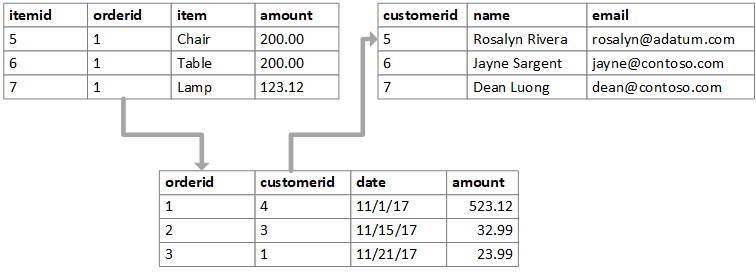
- There are two main kinds of keys; *primary keys* and *foreign keys*.
- A *primary key* uniquely identifies each observation in a particular table.
- A *foreign key* is usually a primary key from one table that appears as a column in another where the first table has a relationship to the second.
### Flight Data
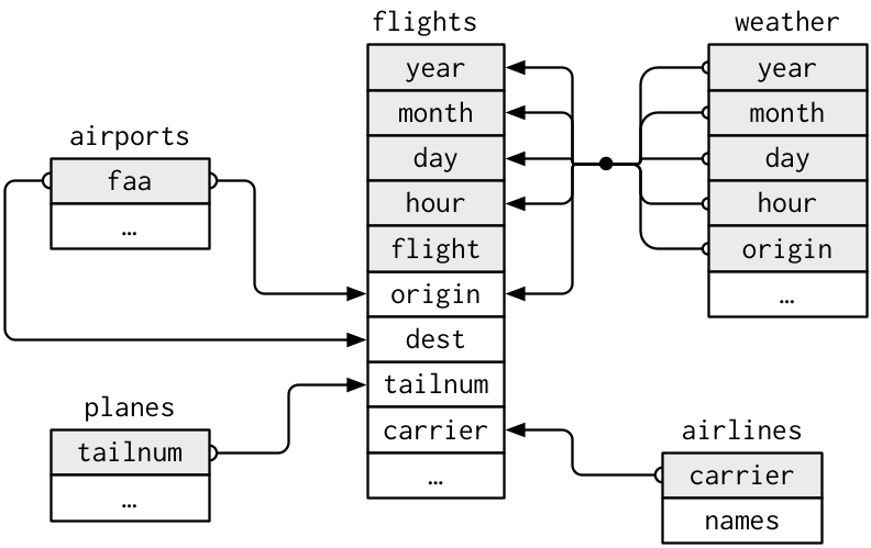
- The `nycflights13` package contains five different datasets that relate to one another:
- `flights`
- `airlines`
- `airports`
- `planes`
- `weather`
- Can you determine the columns (keys) which relate each table to one another?
```{r view_data_flights, exercise=TRUE}
flights
```
```{r view_data_planes, exercise=TRUE}
planes
```
- A relationship diagram of the tables is shown below:
- The primary key in the `flights` dataset is the `tailnum` variable. It is important that you ensure that your primary key is unique for every observation in that table. For example, you wouldn't want to have a dataset of student data with two students having the same student id, if this was the case then the student id wouldn't uniquely identify each observation and would not be a primary key.
- It is good practice to check if a variable you think may be a primary key is unique for all observations. You can do so as follows:
```{r check_key, exercise= TRUE, exercise.eval= FALSE}
planes %>%
count(tailnum) %>%
filter(n > 1)
```
### Exercise
**Exercise: Identify the primary key in the `airlines` table and verify that it is unique for all observations.**
```{r ex-1, exercise= TRUE, exercise.eval= FALSE}
```
```{r ex-1-solution}
airlines %>%
count(carrier) %>%
filter(n > 1)
```
### Primary Key
- The `flights` table lacks a primary key. It is sometimes useful when performing an analysis on relational data to include a primary key if one doesn't exist. You can do this easily using the `cbind()` function.
```{r flights-key, exercise= TRUE, exercise.eval= FALSE}
uniqueID <- c(1:nrow(flights))
flights <- cbind(uniqueID, flights)
```
## Mutating Joins
- We can us the relationships between the tables to combine data from one table to another.
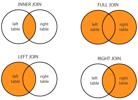
- There are four different kinds of joins:
- An inner join
- A left join
- A right join
- A full join
- An **inner join** will join all observation from table a to table b by matching the keys between the two tables. An inner join will only keep the observations which have matching keys in **both** tables. For example if table a contained keys x, y, z and table b had keys w, x, y, then only the observations with keys x and y would be kept after the join.
- A **left join** keeps all the observations in table a but only keeps the observations from table b which match with the keys from table a. Using the same example as above the observations with keys x, y and z would remain after performing a left join on tables a and b.
- A **right join** is the exact opposite of a left join and will keep all the observations in table b but only the observations from table a which match with the keys from table b.
- A **full join** keeps all observations from both tables.
- Venn diagrams are commonly used to describe these joins:
- For example take the two tables `flights` and `airlines`. The primary key `carrrier` in the `airlines` table is a foreign key in the `flights` table. The left join function can be used to join the two tables as follows:
```{r left_join, exercise = TRUE, exercise.eval = FALSE}
flightsLJ <-
flights %>%
left_join(airlines, by = "carrier")
head(flightsLJ)
```
- The flights table now has 21 columns with the `carrier` variable as the last column. The `carrier` column isn't visible in the R console as the dataset is too wide. To see all the variables use the `View()` function.
### Exercise
**Exercise 2: Create a new smaller `flights` dataset which only contains the `flight`, `origin`, `dest` and `tailnum` variables and call it `flights2`. Then left join the `planes` table to `flights2` so that `flights2` will now contain all the information about the planes used in each flight.**
```{r ex-2, exercise = TRUE, exercise.eval = FALSE}
```
```{r ex-2-solution}
flights2 <- select(flights, flight, origin, dest, tailnum)
flights2 <- flights2 %>%
left_join(planes, by = "tailnum")
head(flights2)
```
- When joining two tables the keys in the two tables may not have the same name in both tables. For example the `airports` table has a variable `faa` that contains the FAA code for each airport. When joining this table to the `flights` table you will notice that the `faa` variable matches to two variables in the `flights` table: `origin` and `dest`. Therefore you must specify the variable you wish to join the tables on as follows:
```{r}
flightsLJ2 <- flights %>%
left_join(airports, c("origin" = "faa"))
head(flightsLJ2)
```
## Filtering Joins
- Filtering joins are similar to mutating joins but they affect the observations in the tables, not the variables.
- There are two different types of filtering joins:
- `semi_join(x, y)`: this keeps all the observations in table x which have a match in table y.
- `anti_join(x, y)`: this keeps all the observations in table x which do **not** have a match in table y.
- For example perhaps you wanted to find out the top five airports with the most outward flights.
When you have this information you then want all the flight information which just relates to flights leaving the five most popular airports. This can be done as follows:
```{r semi_join, exercise = TRUE, exercise.eval = FALSE}
top5origins <- flights %>%
count(origin, sort = TRUE) %>%
head(5)
flightsTop5 <- flights %>%
semi_join(top5origins)
head(flightsTop5)
```
**Exercise: Find the five most popular destinations and obtain the flight data for only the flights going to those five destinations.**
```{r ex-3, exercise = TRUE, exercise.eval = FALSE}
```
```{r ex-3-solution}
top5dest <- flights %>%
count(dest, sort = TRUE) %>%
head(5)
flightsTop5dest <- flights %>%
semi_join(top5dest)
head(flightsTop5dest)
```
**Exercise: Use the anti-join function to find out if any airlines have no flights in the `flights` dataset.**
```{r ex-4, exercise = TRUE, exercise.eval = FALSE}
```
```{r ex-4-solution}
airlines %>%
anti_join(flights, by = "carrier")
```
## Set Operators
- Another method of comparing two datasets is the use of set operators.
- Set operators only work if the two datasets you are comparing have the same variables in each.
- There are three different kinds of set operators:
- `intersect(x, y)`- returns all observations which are in both table x and table y.
- `union(x, y)`- returns the unique observations in table x and y.
- `setdiff(x, y)`- returns all observations in table x but not in y.
```{r, include=is_static, results='asis', echo=FALSE}
cat("# Solutions")
cat("\n### Exercise 1 Solution")
```
```{r ex01-static, include=is_static, eval=is_static}
```
```{r, include=is_static, results='asis', echo=FALSE}
cat("[Back to Exercise 1][Exercise 1] \n")
cat("\n### Exercise 2 Solution")
```
```{r ex02-static, include=is_static, eval=is_static}
```
```{r, include=is_static, results='asis', echo=FALSE}
cat("[Back to Exercise 2][Exercise 2] \n")
cat("\n### Exercise 3 Solution ")
```
```{r ex03-static, include=is_static, eval=is_static}
```
```{r, include=is_static, results='asis', echo=FALSE}
cat("[Back to Exercise 3][Exercise 3] \n")
```