{
"cells": [
{
"cell_type": "markdown",
"metadata": {},
"source": [
"# 11 - Ensemble Methods - Bagging\n",
"\n",
"\n",
"by [Alejandro Correa Bahnsen](albahnsen.com/) and [Jesus Solano](https://github.com/jesugome)\n",
"\n",
"version 1.5, February 2019\n",
"\n",
"## Part of the class [Practical Machine Learning](https://github.com/albahnsen/PracticalMachineLearningClass)\n",
"\n",
"\n",
"\n",
"This notebook is licensed under a [Creative Commons Attribution-ShareAlike 3.0 Unported License](http://creativecommons.org/licenses/by-sa/3.0/deed.en_US). Special thanks goes to [Kevin Markham](https://github.com/justmarkham)"
]
},
{
"cell_type": "markdown",
"metadata": {},
"source": [
"Why are we learning about ensembling?\n",
"\n",
"- Very popular method for improving the predictive performance of machine learning models\n",
"- Provides a foundation for understanding more sophisticated models"
]
},
{
"cell_type": "markdown",
"metadata": {},
"source": [
"## Lesson objectives\n",
"\n",
"Students will be able to:\n",
"\n",
"- Define ensembling and its requirements\n",
"- Identify the two basic methods of ensembling\n",
"- Decide whether manual ensembling is a useful approach for a given problem\n",
"- Explain bagging and how it can be applied to decision trees\n",
"- Explain how out-of-bag error and feature importances are calculated from bagged trees\n",
"- Explain the difference between bagged trees and Random Forests\n",
"- Build and tune a Random Forest model in scikit-learn\n",
"- Decide whether a decision tree or a Random Forest is a better model for a given problem"
]
},
{
"cell_type": "markdown",
"metadata": {},
"source": [
"# Part 1: Introduction"
]
},
{
"cell_type": "markdown",
"metadata": {},
"source": [
"Ensemble learning is a widely studied topic in the machine learning community. The main idea behind \n",
"the ensemble methodology is to combine several individual base classifiers in order to have a \n",
"classifier that outperforms each of them.\n",
"\n",
"Nowadays, ensemble methods are one \n",
"of the most popular and well studied machine learning techniques, and it can be \n",
"noted that since 2009 all the first-place and second-place winners of the KDD-Cup https://www.sigkdd.org/kddcup/ used ensemble methods. The core \n",
"principle in ensemble learning, is to induce random perturbations into the learning procedure in \n",
"order to produce several different base classifiers from a single training set, then combining the \n",
"base classifiers in order to make the final prediction. In order to induce the random permutations \n",
"and therefore create the different base classifiers, several methods have been proposed, in \n",
"particular: \n",
"* bagging\n",
"* pasting\n",
"* random forests \n",
"* random patches \n",
"\n",
"Finally, after the base classifiers \n",
"are trained, they are typically combined using either:\n",
"* majority voting\n",
"* weighted voting \n",
"* stacking\n"
]
},
{
"cell_type": "markdown",
"metadata": {},
"source": [
"There are three main reasons regarding why ensemble \n",
"methods perform better than single models: statistical, computational and representational . First, from a statistical point of view, when the learning set is too \n",
"small, an algorithm can find several good models within the search space, that arise to the same \n",
"performance on the training set $\\mathcal{S}$. Nevertheless, without a validation set, there is \n",
"a risk of choosing the wrong model. The second reason is computational; in general, algorithms \n",
"rely on some local search optimization and may get stuck in a local optima. Then, an ensemble may \n",
"solve this by focusing different algorithms to different spaces across the training set. The last \n",
"reason is representational. In most cases, for a learning set of finite size, the true function \n",
"$f$ cannot be represented by any of the candidate models. By combining several models in an \n",
"ensemble, it may be possible to obtain a model with a larger coverage across the space of \n",
"representable functions."
]
},
{
"cell_type": "markdown",
"metadata": {},
"source": [
""
]
},
{
"cell_type": "markdown",
"metadata": {},
"source": [
"## Example\n",
"\n",
"Let's pretend that instead of building a single model to solve a binary classification problem, you created **five independent models**, and each model was correct about 70% of the time. If you combined these models into an \"ensemble\" and used their majority vote as a prediction, how often would the ensemble be correct?"
]
},
{
"cell_type": "code",
"execution_count": 1,
"metadata": {},
"outputs": [
{
"name": "stdout",
"output_type": "stream",
"text": [
"[0 1 1 1 1 0 0 1 1 1 1 1 1 1 1 1 1 0 1 1]\n",
"[1 1 1 1 1 1 1 0 1 0 0 0 1 1 1 0 1 0 0 0]\n",
"[1 1 1 1 0 1 1 0 0 1 1 1 1 1 1 1 1 0 1 1]\n",
"[1 1 0 0 0 0 1 1 0 1 1 1 1 1 1 0 1 1 1 0]\n",
"[0 0 1 0 0 0 1 0 1 0 0 0 1 1 1 1 1 1 1 1]\n"
]
}
],
"source": [
"import numpy as np\n",
"\n",
"# set a seed for reproducibility\n",
"np.random.seed(1234)\n",
"\n",
"# generate 1000 random numbers (between 0 and 1) for each model, representing 1000 observations\n",
"mod1 = np.random.rand(1000)\n",
"mod2 = np.random.rand(1000)\n",
"mod3 = np.random.rand(1000)\n",
"mod4 = np.random.rand(1000)\n",
"mod5 = np.random.rand(1000)\n",
"\n",
"# each model independently predicts 1 (the \"correct response\") if random number was at least 0.3\n",
"preds1 = np.where(mod1 > 0.3, 1, 0)\n",
"preds2 = np.where(mod2 > 0.3, 1, 0)\n",
"preds3 = np.where(mod3 > 0.3, 1, 0)\n",
"preds4 = np.where(mod4 > 0.3, 1, 0)\n",
"preds5 = np.where(mod5 > 0.3, 1, 0)\n",
"\n",
"# print the first 20 predictions from each model\n",
"print(preds1[:20])\n",
"print(preds2[:20])\n",
"print(preds3[:20])\n",
"print(preds4[:20])\n",
"print(preds5[:20])"
]
},
{
"cell_type": "code",
"execution_count": 2,
"metadata": {},
"outputs": [
{
"name": "stdout",
"output_type": "stream",
"text": [
"[1 1 1 1 0 0 1 0 1 1 1 1 1 1 1 1 1 0 1 1]\n"
]
}
],
"source": [
"# average the predictions and then round to 0 or 1\n",
"ensemble_preds = np.round((preds1 + preds2 + preds3 + preds4 + preds5)/5.0).astype(int)\n",
"\n",
"# print the ensemble's first 20 predictions\n",
"print(ensemble_preds[:20])"
]
},
{
"cell_type": "code",
"execution_count": 3,
"metadata": {},
"outputs": [
{
"name": "stdout",
"output_type": "stream",
"text": [
"0.713\n",
"0.665\n",
"0.717\n",
"0.712\n",
"0.687\n"
]
}
],
"source": [
"# how accurate was each individual model?\n",
"print(preds1.mean())\n",
"print(preds2.mean())\n",
"print(preds3.mean())\n",
"print(preds4.mean())\n",
"print(preds5.mean())"
]
},
{
"cell_type": "code",
"execution_count": 4,
"metadata": {},
"outputs": [
{
"name": "stdout",
"output_type": "stream",
"text": [
"0.841\n"
]
}
],
"source": [
"# how accurate was the ensemble?\n",
"print(ensemble_preds.mean())"
]
},
{
"cell_type": "markdown",
"metadata": {},
"source": [
"**Note:** As you add more models to the voting process, the probability of error decreases, which is known as [Condorcet's Jury Theorem](http://en.wikipedia.org/wiki/Condorcet%27s_jury_theorem)."
]
},
{
"cell_type": "markdown",
"metadata": {},
"source": [
"## What is ensembling?\n",
"\n",
"**Ensemble learning (or \"ensembling\")** is the process of combining several predictive models in order to produce a combined model that is more accurate than any individual model.\n",
"\n",
"- **Regression:** take the average of the predictions\n",
"- **Classification:** take a vote and use the most common prediction, or take the average of the predicted probabilities\n",
"\n",
"For ensembling to work well, the models must have the following characteristics:\n",
"\n",
"- **Accurate:** they outperform the null model\n",
"- **Independent:** their predictions are generated using different processes\n",
"\n",
"**The big idea:** If you have a collection of individually imperfect (and independent) models, the \"one-off\" mistakes made by each model are probably not going to be made by the rest of the models, and thus the mistakes will be discarded when averaging the models.\n",
"\n",
"There are two basic **methods for ensembling:**\n",
"\n",
"- Manually ensemble your individual models\n",
"- Use a model that ensembles for you"
]
},
{
"cell_type": "markdown",
"metadata": {},
"source": [
"### Theoretical performance of an ensemble\n",
" If we assume that each one of the $T$ base classifiers has a probability $\\rho$ of \n",
" being correct, the probability of an ensemble making the correct decision, assuming independence, \n",
" denoted by $P_c$, can be calculated using the binomial distribution\n",
"\n",
"$$P_c = \\sum_{j>T/2}^{T} {{T}\\choose{j}} \\rho^j(1-\\rho)^{T-j}.$$\n",
"\n",
" Furthermore, as shown, if $T\\ge3$ then:\n",
"\n",
"$$\n",
" \\lim_{T \\to \\infty} P_c= \\begin{cases} \n",
" 1 &\\mbox{if } \\rho>0.5 \\\\ \n",
" 0 &\\mbox{if } \\rho<0.5 \\\\ \n",
" 0.5 &\\mbox{if } \\rho=0.5 ,\n",
" \\end{cases}\n",
"$$\n",
"\tleading to the conclusion that \n",
"$$\n",
" \\rho \\ge 0.5 \\quad \\text{and} \\quad T\\ge3 \\quad \\Rightarrow \\quad P_c\\ge \\rho.\n",
"$$"
]
},
{
"cell_type": "markdown",
"metadata": {
"collapsed": true
},
"source": [
"# Part 2: Manual ensembling\n",
"\n",
"What makes a good manual ensemble?\n",
"\n",
"- Different types of **models**\n",
"- Different combinations of **features**\n",
"- Different **tuning parameters**"
]
},
{
"cell_type": "markdown",
"metadata": {},
"source": [
"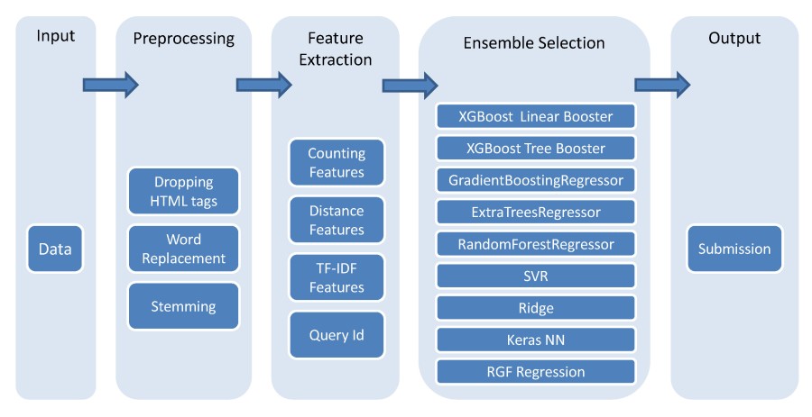\n",
"\n",
"*Machine learning flowchart created by the [winner](https://github.com/ChenglongChen/Kaggle_CrowdFlower) of Kaggle's [CrowdFlower competition](https://www.kaggle.com/c/crowdflower-search-relevance)*"
]
},
{
"cell_type": "code",
"execution_count": 5,
"metadata": {},
"outputs": [],
"source": [
"# read in and prepare the vehicle training data\n",
"import pandas as pd\n",
"url = 'https://raw.githubusercontent.com/albahnsen/PracticalMachineLearningClass/master/datasets/vehicles_train.csv'\n",
"train = pd.read_csv(url)\n",
"train['vtype'] = train.vtype.map({'car':0, 'truck':1})\n",
"# read in and prepare the vehicle testing data\n",
"url = 'https://raw.githubusercontent.com/albahnsen/PracticalMachineLearningClass/master/datasets/vehicles_test.csv'\n",
"test = pd.read_csv(url)\n",
"test['vtype'] = test.vtype.map({'car':0, 'truck':1})"
]
},
{
"cell_type": "code",
"execution_count": 6,
"metadata": {},
"outputs": [
{
"data": {
"text/html": [
"
\n",
"\n",
"
\n",
" \n",
"
\n",
"
\n",
"
price
\n",
"
year
\n",
"
miles
\n",
"
doors
\n",
"
vtype
\n",
"
\n",
" \n",
" \n",
"
\n",
"
0
\n",
"
22000
\n",
"
2012
\n",
"
13000
\n",
"
2
\n",
"
0
\n",
"
\n",
"
\n",
"
1
\n",
"
14000
\n",
"
2010
\n",
"
30000
\n",
"
2
\n",
"
0
\n",
"
\n",
"
\n",
"
2
\n",
"
13000
\n",
"
2010
\n",
"
73500
\n",
"
4
\n",
"
0
\n",
"
\n",
"
\n",
"
3
\n",
"
9500
\n",
"
2009
\n",
"
78000
\n",
"
4
\n",
"
0
\n",
"
\n",
"
\n",
"
4
\n",
"
9000
\n",
"
2007
\n",
"
47000
\n",
"
4
\n",
"
0
\n",
"
\n",
" \n",
"
\n",
"
"
],
"text/plain": [
" price year miles doors vtype\n",
"0 22000 2012 13000 2 0\n",
"1 14000 2010 30000 2 0\n",
"2 13000 2010 73500 4 0\n",
"3 9500 2009 78000 4 0\n",
"4 9000 2007 47000 4 0"
]
},
"execution_count": 6,
"metadata": {},
"output_type": "execute_result"
}
],
"source": [
"train.head()"
]
},
{
"cell_type": "markdown",
"metadata": {},
"source": [
"### Train different models"
]
},
{
"cell_type": "code",
"execution_count": 7,
"metadata": {},
"outputs": [],
"source": [
"from sklearn.linear_model import LinearRegression\n",
"from sklearn.tree import DecisionTreeRegressor\n",
"from sklearn.naive_bayes import GaussianNB\n",
"from sklearn.neighbors import KNeighborsRegressor\n",
"\n",
"models = {'lr': LinearRegression(),\n",
" 'dt': DecisionTreeRegressor(),\n",
" 'nb': GaussianNB(),\n",
" 'kn': KNeighborsRegressor()}"
]
},
{
"cell_type": "code",
"execution_count": 8,
"metadata": {},
"outputs": [],
"source": [
"# Train all the models\n",
"X_train = train.iloc[:, 1:]\n",
"X_test = test.iloc[:, 1:]\n",
"y_train = train.price\n",
"y_test = test.price\n",
"\n",
"for model in models.keys():\n",
" models[model].fit(X_train, y_train)"
]
},
{
"cell_type": "code",
"execution_count": 9,
"metadata": {},
"outputs": [],
"source": [
"# predict test for each model\n",
"y_pred = pd.DataFrame(index=test.index, columns=models.keys())\n",
"for model in models.keys():\n",
" y_pred[model] = models[model].predict(X_test)\n",
" "
]
},
{
"cell_type": "code",
"execution_count": 10,
"metadata": {},
"outputs": [
{
"name": "stdout",
"output_type": "stream",
"text": [
"lr 2138.3579028745116\n",
"dt 1414.213562373095\n",
"nb 5477.2255750516615\n",
"kn 1671.3268182295567\n"
]
}
],
"source": [
"# Evaluate each model\n",
"from sklearn.metrics import mean_squared_error\n",
"\n",
"for model in models.keys():\n",
" print(model,np.sqrt(mean_squared_error(y_pred[model], y_test)))"
]
},
{
"cell_type": "markdown",
"metadata": {},
"source": [
"### Evaluate the error of the mean of the predictions"
]
},
{
"cell_type": "code",
"execution_count": 11,
"metadata": {},
"outputs": [
{
"data": {
"text/plain": [
"1193.164765760328"
]
},
"execution_count": 11,
"metadata": {},
"output_type": "execute_result"
}
],
"source": [
"np.sqrt(mean_squared_error(y_pred.mean(axis=1), y_test))"
]
},
{
"cell_type": "markdown",
"metadata": {},
"source": [
"## Comparing manual ensembling with a single model approach\n",
"\n",
"**Advantages of manual ensembling:**\n",
"\n",
"- Increases predictive accuracy\n",
"- Easy to get started\n",
"\n",
"**Disadvantages of manual ensembling:**\n",
"\n",
"- Decreases interpretability\n",
"- Takes longer to train\n",
"- Takes longer to predict\n",
"- More complex to automate and maintain\n",
"- Small gains in accuracy may not be worth the added complexity"
]
},
{
"cell_type": "markdown",
"metadata": {},
"source": [
"# Part 3: Bagging\n",
"\n",
"The primary weakness of **decision trees** is that they don't tend to have the best predictive accuracy. This is partially due to **high variance**, meaning that different splits in the training data can lead to very different trees.\n",
"\n",
"**Bagging** is a general purpose procedure for reducing the variance of a machine learning method, but is particularly useful for decision trees. Bagging is short for **bootstrap aggregation**, meaning the aggregation of bootstrap samples.\n",
"\n",
"What is a **bootstrap sample**? A random sample with replacement:"
]
},
{
"cell_type": "code",
"execution_count": 12,
"metadata": {},
"outputs": [
{
"name": "stdout",
"output_type": "stream",
"text": [
"[ 1 2 3 4 5 6 7 8 9 10 11 12 13 14 15 16 17 18 19 20]\n",
"[ 6 12 13 9 10 12 6 16 1 17 2 13 8 14 7 19 6 19 12 11]\n"
]
}
],
"source": [
"# set a seed for reproducibility\n",
"np.random.seed(1)\n",
"\n",
"# create an array of 1 through 20\n",
"nums = np.arange(1, 21)\n",
"print(nums)\n",
"\n",
"# sample that array 20 times with replacement\n",
"print(np.random.choice(a=nums, size=20, replace=True))"
]
},
{
"cell_type": "markdown",
"metadata": {},
"source": [
"**How does bagging work (for decision trees)?**\n",
"\n",
"1. Grow B trees using B bootstrap samples from the training data.\n",
"2. Train each tree on its bootstrap sample and make predictions.\n",
"3. Combine the predictions:\n",
" - Average the predictions for **regression trees**\n",
" - Take a vote for **classification trees**\n",
"\n",
"Notes:\n",
"\n",
"- **Each bootstrap sample** should be the same size as the original training set.\n",
"- **B** should be a large enough value that the error seems to have \"stabilized\".\n",
"- The trees are **grown deep** so that they have low bias/high variance.\n",
"\n",
"Bagging increases predictive accuracy by **reducing the variance**, similar to how cross-validation reduces the variance associated with train/test split (for estimating out-of-sample error) by splitting many times an averaging the results.\n"
]
},
{
"cell_type": "code",
"execution_count": 13,
"metadata": {},
"outputs": [
{
"data": {
"text/plain": [
"[array([13, 2, 12, 2, 6, 1, 3, 10, 11, 9, 6, 1, 0, 1]),\n",
" array([ 9, 0, 0, 9, 3, 13, 4, 0, 0, 4, 1, 7, 3, 2]),\n",
" array([ 4, 7, 2, 4, 8, 13, 0, 7, 9, 3, 12, 12, 4, 6]),\n",
" array([ 1, 5, 6, 11, 2, 1, 12, 8, 3, 10, 5, 0, 11, 2]),\n",
" array([10, 10, 6, 13, 2, 4, 11, 11, 13, 12, 4, 6, 13, 3]),\n",
" array([10, 0, 6, 4, 7, 11, 6, 7, 1, 11, 10, 5, 7, 9]),\n",
" array([ 2, 4, 8, 1, 12, 2, 1, 1, 3, 12, 5, 9, 0, 8]),\n",
" array([11, 1, 6, 3, 3, 11, 5, 9, 7, 9, 2, 3, 11, 3]),\n",
" array([ 3, 8, 6, 9, 7, 6, 3, 9, 6, 12, 6, 11, 6, 1]),\n",
" array([13, 10, 3, 4, 3, 1, 13, 0, 5, 8, 13, 6, 11, 8])]"
]
},
"execution_count": 13,
"metadata": {},
"output_type": "execute_result"
}
],
"source": [
"# set a seed for reproducibility\n",
"np.random.seed(123)\n",
"\n",
"n_samples = train.shape[0]\n",
"n_B = 10\n",
"\n",
"# create ten bootstrap samples (will be used to select rows from the DataFrame)\n",
"samples = [np.random.choice(a=n_samples, size=n_samples, replace=True) for _ in range(1, n_B +1 )]\n",
"samples"
]
},
{
"cell_type": "code",
"execution_count": 14,
"metadata": {},
"outputs": [
{
"data": {
"text/html": [
"
\n",
"\n",
"
\n",
" \n",
"
\n",
"
\n",
"
price
\n",
"
year
\n",
"
miles
\n",
"
doors
\n",
"
vtype
\n",
"
\n",
" \n",
" \n",
"
\n",
"
13
\n",
"
1300
\n",
"
1997
\n",
"
138000
\n",
"
4
\n",
"
0
\n",
"
\n",
"
\n",
"
2
\n",
"
13000
\n",
"
2010
\n",
"
73500
\n",
"
4
\n",
"
0
\n",
"
\n",
"
\n",
"
12
\n",
"
1800
\n",
"
1999
\n",
"
163000
\n",
"
2
\n",
"
1
\n",
"
\n",
"
\n",
"
2
\n",
"
13000
\n",
"
2010
\n",
"
73500
\n",
"
4
\n",
"
0
\n",
"
\n",
"
\n",
"
6
\n",
"
3000
\n",
"
2004
\n",
"
177000
\n",
"
4
\n",
"
0
\n",
"
\n",
"
\n",
"
1
\n",
"
14000
\n",
"
2010
\n",
"
30000
\n",
"
2
\n",
"
0
\n",
"
\n",
"
\n",
"
3
\n",
"
9500
\n",
"
2009
\n",
"
78000
\n",
"
4
\n",
"
0
\n",
"
\n",
"
\n",
"
10
\n",
"
2500
\n",
"
2003
\n",
"
190000
\n",
"
2
\n",
"
1
\n",
"
\n",
"
\n",
"
11
\n",
"
5000
\n",
"
2001
\n",
"
62000
\n",
"
4
\n",
"
0
\n",
"
\n",
"
\n",
"
9
\n",
"
1900
\n",
"
2003
\n",
"
160000
\n",
"
4
\n",
"
0
\n",
"
\n",
"
\n",
"
6
\n",
"
3000
\n",
"
2004
\n",
"
177000
\n",
"
4
\n",
"
0
\n",
"
\n",
"
\n",
"
1
\n",
"
14000
\n",
"
2010
\n",
"
30000
\n",
"
2
\n",
"
0
\n",
"
\n",
"
\n",
"
0
\n",
"
22000
\n",
"
2012
\n",
"
13000
\n",
"
2
\n",
"
0
\n",
"
\n",
"
\n",
"
1
\n",
"
14000
\n",
"
2010
\n",
"
30000
\n",
"
2
\n",
"
0
\n",
"
\n",
" \n",
"
\n",
"
"
],
"text/plain": [
" price year miles doors vtype\n",
"13 1300 1997 138000 4 0\n",
"2 13000 2010 73500 4 0\n",
"12 1800 1999 163000 2 1\n",
"2 13000 2010 73500 4 0\n",
"6 3000 2004 177000 4 0\n",
"1 14000 2010 30000 2 0\n",
"3 9500 2009 78000 4 0\n",
"10 2500 2003 190000 2 1\n",
"11 5000 2001 62000 4 0\n",
"9 1900 2003 160000 4 0\n",
"6 3000 2004 177000 4 0\n",
"1 14000 2010 30000 2 0\n",
"0 22000 2012 13000 2 0\n",
"1 14000 2010 30000 2 0"
]
},
"execution_count": 14,
"metadata": {},
"output_type": "execute_result"
}
],
"source": [
"# show the rows for the first decision tree\n",
"train.iloc[samples[0], :]"
]
},
{
"cell_type": "markdown",
"metadata": {},
"source": [
" Build one tree for each sample"
]
},
{
"cell_type": "code",
"execution_count": 15,
"metadata": {},
"outputs": [],
"source": [
"from sklearn.tree import DecisionTreeRegressor\n",
"\n",
"# grow each tree deep\n",
"treereg = DecisionTreeRegressor(max_depth=None, random_state=123)\n",
"\n",
"# DataFrame for storing predicted price from each tree\n",
"y_pred = pd.DataFrame(index=test.index, columns=[list(range(n_B))])\n",
"\n",
"# grow one tree for each bootstrap sample and make predictions on testing data\n",
"for i, sample in enumerate(samples):\n",
" X_train = train.iloc[sample, 1:]\n",
" y_train = train.iloc[sample, 0]\n",
" treereg.fit(X_train, y_train)\n",
" y_pred[i] = treereg.predict(X_test)"
]
},
{
"cell_type": "code",
"execution_count": 16,
"metadata": {},
"outputs": [
{
"data": {
"text/html": [
"
\n",
"\n",
"
\n",
" \n",
"
\n",
"
\n",
"
0
\n",
"
1
\n",
"
2
\n",
"
3
\n",
"
4
\n",
"
5
\n",
"
6
\n",
"
7
\n",
"
8
\n",
"
9
\n",
"
\n",
" \n",
" \n",
"
\n",
"
0
\n",
"
1300.0
\n",
"
1300.0
\n",
"
3000.0
\n",
"
4000.0
\n",
"
1300.0
\n",
"
4000.0
\n",
"
4000.0
\n",
"
4000.0
\n",
"
3000.0
\n",
"
4000.0
\n",
"
\n",
"
\n",
"
1
\n",
"
5000.0
\n",
"
1300.0
\n",
"
3000.0
\n",
"
5000.0
\n",
"
5000.0
\n",
"
5000.0
\n",
"
4000.0
\n",
"
5000.0
\n",
"
5000.0
\n",
"
5000.0
\n",
"
\n",
"
\n",
"
2
\n",
"
14000.0
\n",
"
13000.0
\n",
"
13000.0
\n",
"
13000.0
\n",
"
13000.0
\n",
"
14000.0
\n",
"
13000.0
\n",
"
13000.0
\n",
"
9500.0
\n",
"
9000.0
\n",
"
\n",
" \n",
"
\n",
"
"
],
"text/plain": [
" 0 1 2 3 4 5 6 7 \\\n",
"0 1300.0 1300.0 3000.0 4000.0 1300.0 4000.0 4000.0 4000.0 \n",
"1 5000.0 1300.0 3000.0 5000.0 5000.0 5000.0 4000.0 5000.0 \n",
"2 14000.0 13000.0 13000.0 13000.0 13000.0 14000.0 13000.0 13000.0 \n",
"\n",
" 8 9 \n",
"0 3000.0 4000.0 \n",
"1 5000.0 5000.0 \n",
"2 9500.0 9000.0 "
]
},
"execution_count": 16,
"metadata": {},
"output_type": "execute_result"
}
],
"source": [
"y_pred"
]
},
{
"cell_type": "markdown",
"metadata": {},
"source": [
"Results of each tree"
]
},
{
"cell_type": "code",
"execution_count": 17,
"metadata": {},
"outputs": [
{
"name": "stdout",
"output_type": "stream",
"text": [
"0 1621.7274740226856\n",
"1 2942.7877939124323\n",
"2 1825.7418583505537\n",
"3 1000.0\n",
"4 1276.7145334803704\n",
"5 1414.213562373095\n",
"6 1414.213562373095\n",
"7 1000.0\n",
"8 1554.5631755148024\n",
"9 1914.854215512676\n"
]
}
],
"source": [
"for i in range(n_B):\n",
" print(i, np.sqrt(mean_squared_error(y_pred[i], y_test)))"
]
},
{
"cell_type": "markdown",
"metadata": {},
"source": [
"Results of the ensemble"
]
},
{
"cell_type": "code",
"execution_count": 18,
"metadata": {},
"outputs": [
{
"data": {
"text/plain": [
"0 2990.0\n",
"1 4330.0\n",
"2 12450.0\n",
"dtype: float64"
]
},
"execution_count": 18,
"metadata": {},
"output_type": "execute_result"
}
],
"source": [
"y_pred.mean(axis=1)"
]
},
{
"cell_type": "code",
"execution_count": 19,
"metadata": {},
"outputs": [
{
"data": {
"text/plain": [
"998.5823284370031"
]
},
"execution_count": 19,
"metadata": {},
"output_type": "execute_result"
}
],
"source": [
"np.sqrt(mean_squared_error(y_test, y_pred.mean(axis=1)))"
]
},
{
"cell_type": "markdown",
"metadata": {},
"source": [
"## Bagged decision trees in scikit-learn (with B=500)"
]
},
{
"cell_type": "code",
"execution_count": 20,
"metadata": {},
"outputs": [],
"source": [
"# define the training and testing sets\n",
"X_train = train.iloc[:, 1:]\n",
"y_train = train.iloc[:, 0]\n",
"X_test = test.iloc[:, 1:]\n",
"y_test = test.iloc[:, 0]"
]
},
{
"cell_type": "code",
"execution_count": 21,
"metadata": {},
"outputs": [
{
"name": "stderr",
"output_type": "stream",
"text": [
"C:\\Users\\albah\\Anaconda3\\lib\\site-packages\\sklearn\\ensemble\\weight_boosting.py:29: DeprecationWarning: numpy.core.umath_tests is an internal NumPy module and should not be imported. It will be removed in a future NumPy release.\n",
" from numpy.core.umath_tests import inner1d\n"
]
}
],
"source": [
"# instruct BaggingRegressor to use DecisionTreeRegressor as the \"base estimator\"\n",
"from sklearn.ensemble import BaggingRegressor\n",
"bagreg = BaggingRegressor(DecisionTreeRegressor(), n_estimators=500, \n",
" bootstrap=True, oob_score=True, random_state=1)"
]
},
{
"cell_type": "code",
"execution_count": 22,
"metadata": {},
"outputs": [
{
"data": {
"text/plain": [
"array([ 3344.2, 5395. , 12902. ])"
]
},
"execution_count": 22,
"metadata": {},
"output_type": "execute_result"
}
],
"source": [
"# fit and predict\n",
"bagreg.fit(X_train, y_train)\n",
"y_pred = bagreg.predict(X_test)\n",
"y_pred"
]
},
{
"cell_type": "code",
"execution_count": 23,
"metadata": {},
"outputs": [
{
"data": {
"text/plain": [
"657.8000304043775"
]
},
"execution_count": 23,
"metadata": {},
"output_type": "execute_result"
}
],
"source": [
"# calculate RMSE\n",
"np.sqrt(mean_squared_error(y_test, y_pred))"
]
},
{
"cell_type": "markdown",
"metadata": {},
"source": [
"## Estimating out-of-sample error\n",
"\n",
"For bagged models, out-of-sample error can be estimated without using **train/test split** or **cross-validation**!\n",
"\n",
"On average, each bagged tree uses about **two-thirds** of the observations. For each tree, the **remaining observations** are called \"out-of-bag\" observations."
]
},
{
"cell_type": "code",
"execution_count": 24,
"metadata": {},
"outputs": [
{
"data": {
"text/plain": [
"array([13, 2, 12, 2, 6, 1, 3, 10, 11, 9, 6, 1, 0, 1])"
]
},
"execution_count": 24,
"metadata": {},
"output_type": "execute_result"
}
],
"source": [
"# show the first bootstrap sample\n",
"samples[0]"
]
},
{
"cell_type": "code",
"execution_count": 25,
"metadata": {},
"outputs": [
{
"name": "stdout",
"output_type": "stream",
"text": [
"{0, 1, 2, 3, 6, 9, 10, 11, 12, 13}\n",
"{0, 1, 2, 3, 4, 7, 9, 13}\n",
"{0, 2, 3, 4, 6, 7, 8, 9, 12, 13}\n",
"{0, 1, 2, 3, 5, 6, 8, 10, 11, 12}\n",
"{2, 3, 4, 6, 10, 11, 12, 13}\n",
"{0, 1, 4, 5, 6, 7, 9, 10, 11}\n",
"{0, 1, 2, 3, 4, 5, 8, 9, 12}\n",
"{1, 2, 3, 5, 6, 7, 9, 11}\n",
"{1, 3, 6, 7, 8, 9, 11, 12}\n",
"{0, 1, 3, 4, 5, 6, 8, 10, 11, 13}\n"
]
}
],
"source": [
"# show the \"in-bag\" observations for each sample\n",
"for sample in samples:\n",
" print(set(sample))"
]
},
{
"cell_type": "code",
"execution_count": 26,
"metadata": {},
"outputs": [
{
"name": "stdout",
"output_type": "stream",
"text": [
"[4, 5, 7, 8]\n",
"[5, 6, 8, 10, 11, 12]\n",
"[1, 5, 10, 11]\n",
"[4, 7, 9, 13]\n",
"[0, 1, 5, 7, 8, 9]\n",
"[2, 3, 8, 12, 13]\n",
"[6, 7, 10, 11, 13]\n",
"[0, 4, 8, 10, 12, 13]\n",
"[0, 2, 4, 5, 10, 13]\n",
"[2, 7, 9, 12]\n"
]
}
],
"source": [
"# show the \"out-of-bag\" observations for each sample\n",
"for sample in samples:\n",
" print(sorted(set(range(n_samples)) - set(sample)))"
]
},
{
"cell_type": "markdown",
"metadata": {},
"source": [
"How to calculate **\"out-of-bag error\":**\n",
"\n",
"1. For every observation in the training data, predict its response value using **only** the trees in which that observation was out-of-bag. Average those predictions (for regression) or take a vote (for classification).\n",
"2. Compare all predictions to the actual response values in order to compute the out-of-bag error.\n",
"\n",
"When B is sufficiently large, the **out-of-bag error** is an accurate estimate of **out-of-sample error**."
]
},
{
"cell_type": "code",
"execution_count": 27,
"metadata": {},
"outputs": [
{
"data": {
"text/plain": [
"0.7986955133989982"
]
},
"execution_count": 27,
"metadata": {},
"output_type": "execute_result"
}
],
"source": [
"# compute the out-of-bag R-squared score (not MSE, unfortunately!) for B=500\n",
"bagreg.oob_score_"
]
},
{
"cell_type": "markdown",
"metadata": {},
"source": [
"## Estimating feature importance\n",
"\n",
"Bagging increases **predictive accuracy**, but decreases **model interpretability** because it's no longer possible to visualize the tree to understand the importance of each feature.\n",
"\n",
"However, we can still obtain an overall summary of **feature importance** from bagged models:\n",
"\n",
"- **Bagged regression trees:** calculate the total amount that **MSE** is decreased due to splits over a given feature, averaged over all trees\n",
"- **Bagged classification trees:** calculate the total amount that **Gini index** is decreased due to splits over a given feature, averaged over all trees"
]
},
{
"cell_type": "markdown",
"metadata": {},
"source": [
"# Part 4: Combination of classifiers - Majority Voting"
]
},
{
"cell_type": "markdown",
"metadata": {},
"source": [
" The most typical form of an ensemble is made by combining $T$ different base classifiers.\n",
" Each base classifier $M(\\mathcal{S}_j)$ is trained by applying algorithm $M$ to a random subset \n",
" $\\mathcal{S}_j$ of the training set $\\mathcal{S}$. \n",
" For simplicity we define $M_j \\equiv M(\\mathcal{S}_j)$ for $j=1,\\dots,T$, and \n",
" $\\mathcal{M}=\\{M_j\\}_{j=1}^{T}$ a set of base classifiers.\n",
" Then, these models are combined using majority voting to create the ensemble $H$ as follows\n",
" $$\n",
" f_{mv}(\\mathcal{S},\\mathcal{M}) = max_{c \\in \\{0,1\\}} \\sum_{j=1}^T \n",
" \\mathbf{1}_c(M_j(\\mathcal{S})).\n",
" $$\n"
]
},
{
"cell_type": "code",
"execution_count": 28,
"metadata": {},
"outputs": [],
"source": [
"# read in and prepare the churn data\n",
"# Download the dataset\n",
"import pandas as pd\n",
"import numpy as np\n",
"\n",
"url = 'https://raw.githubusercontent.com/albahnsen/PracticalMachineLearningClass/master/datasets/churn.csv'\n",
"data = pd.read_csv(url)\n",
"\n",
"# Create X and y\n",
"\n",
"# Select only the numeric features\n",
"X = data.iloc[:, [1,2,6,7,8,9,10]].astype(np.float)\n",
"# Convert bools to floats\n",
"X = X.join((data.iloc[:, [4,5]] == 'no').astype(np.float))\n",
"\n",
"y = (data.iloc[:, -1] == 'True.').astype(np.int)"
]
},
{
"cell_type": "code",
"execution_count": 29,
"metadata": {},
"outputs": [
{
"data": {
"text/html": [
"