---
title: |
{width="125"} {width="100"} {width="350"} \
Microbiome data integration workflow for population cohort studies
subtitle: Package demo
output:
html_document:
code_folding: show
---
```{r setup, message=FALSE, class.source = 'fold-hide'}
# Define the directory names of the dependent data
directories <- c("data", "figures")
# Check if any of the directories is missing
if (any(!dir.exists(directories))) {
# Define the URL of the tar.gz file created with `tar -cvf EuroBioC2023.tar.gz data/ figures/ workflow.html`
url <- "https://raw.githubusercontent.com/microbiome/outreach/main/demo/EuroBioC2023/EuroBioC2023.tar.gz"
# Extract the local file name from the URL
local_file <- basename(url)
# Download the file from the URL
download.file(url, local_file)
# Untar the downloaded file in the current directory
untar(local_file, exdir = ".")
}
# List of packages that we need
packages <- c(
"ANCOMBC", "ComplexHeatmap", "ggplot2", "knitr", "mia", "miaViz", "dplyr",
"tidyr", "scater", "knitr")
# Get packages that are already installed installed
packages_already_installed <- packages[ packages %in% installed.packages() ]
# Get packages that need to be installed
packages_need_to_install <- setdiff( packages, packages_already_installed )
# Loads BiocManager into the session. Install it if it not already installed.
if( !require("BiocManager") ){
install.packages("BiocManager")
library("BiocManager")
}
# If there are packages that need to be installed, installs them with BiocManager
# Updates old packages.
if( length(packages_need_to_install) > 0 ) {
install(packages_need_to_install, ask = FALSE)
}
# Load all packages into session. Stop if there are packages that were not
# successfully loaded
if( any(!sapply(packages, require, character.only = TRUE)) ){
stop("Error in loading packages into the session.")
}
################################################################################
# Additional setup
# Set chunk options
opts_chunk$set(message = FALSE, warning = FALSE)
# Set black and white theme for figures, and Arial font
theme <- theme_bw() +
theme(
text = element_text(family = "Arial"),
panel.border = element_blank(),
panel.grid.major = element_blank(),
panel.grid.minor = element_blank(),
axis.line = element_line(colour = "black")
)
theme_set(theme)
```
 #### EuroBioC2023
- European Bioconductor Conference 2023
- Ghent, Belgium
- September 21, 2023; 13:30 (CEST)
- **See the poster also (miaverse -- microbiome analytics framework in SummarizedExperiment family)!**
#### Presenter information
All authors are affiliated to [Turku Data Science Group in University of Turku, Finland.](https://datascience.utu.fi/)
#### EuroBioC2023
- European Bioconductor Conference 2023
- Ghent, Belgium
- September 21, 2023; 13:30 (CEST)
- **See the poster also (miaverse -- microbiome analytics framework in SummarizedExperiment family)!**
#### Presenter information
All authors are affiliated to [Turku Data Science Group in University of Turku, Finland.](https://datascience.utu.fi/)  - **Tuomas Borman -- doctoral researcher**
- Chouaib Benchraka -- doctoral researcher
- Leo Lahti -- group leader
------------------------------------------------------------------------
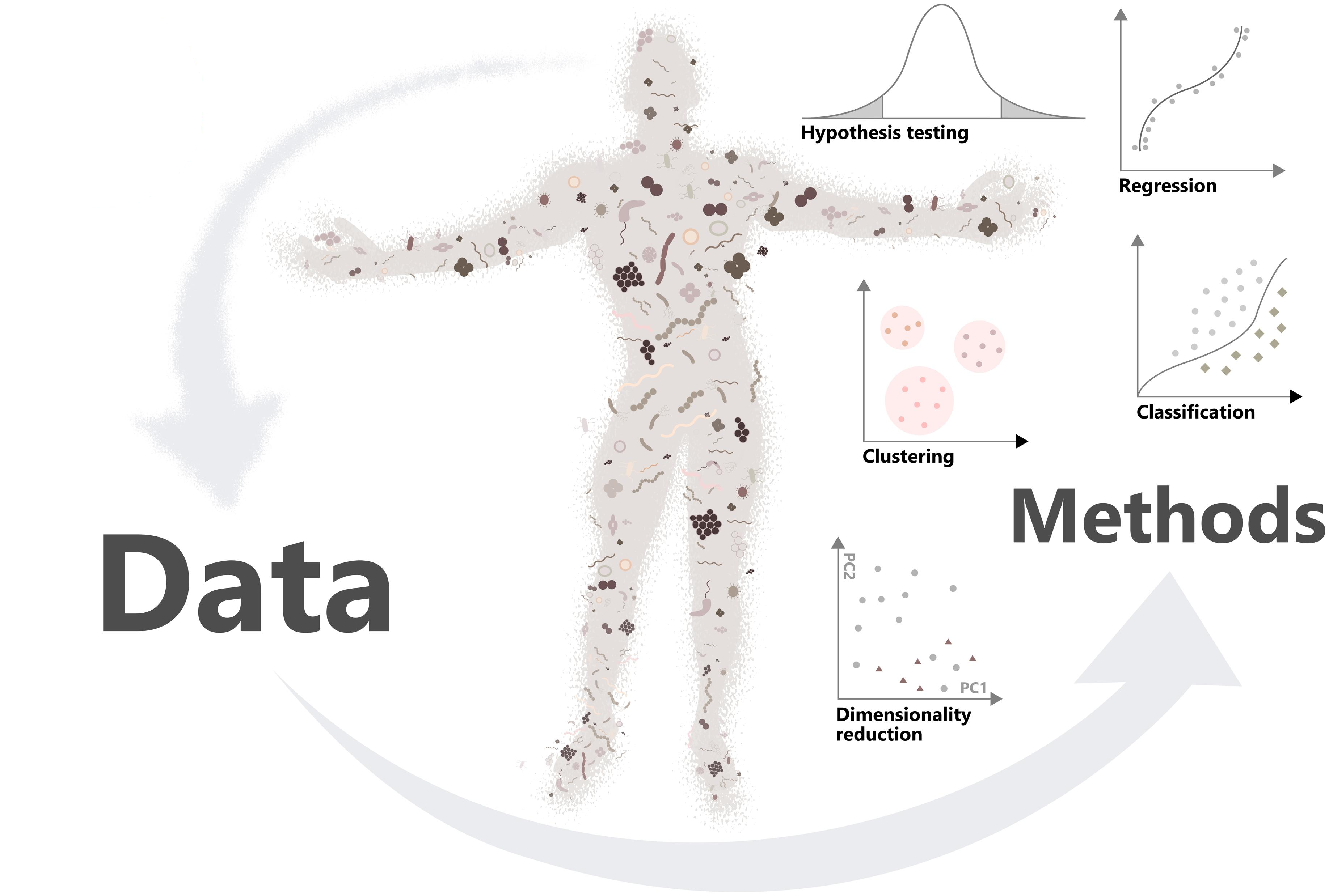
## Learning goals
1. Microbiome research studies interactions between microbes (and human, environment...)
2. Big data requires efficient tools to manipulate the data
3. miaverse is a (Tree)SummarizedExperiment framework for microbiome analytics
{width="400"}
## Motivation
### Microbiome research
- Microbiome is a composition of microbes in well-defined area (gut, skin, mouth...)
- Bilateral interaction between human and microbiome --> affects both health and disease.
- The research is based on sequencing (characterization of genes and species).
- Nowadays, multiomics approach is more common (integration of taxonomy information with metabolite data, for example)
- Computational methods are the new microscope
- The research has expanded rapidly in previous years
```{r pubmed_fig, fig.width=6, fig.cap="PubMed publications per year with a search term 'microbiome' (fetched: Sep 5, 2023)", class.source = 'fold-hide'}
# Plot publication graph
path <- "data/PubMed_Timeline_Results_by_Year.csv"
df <- read.csv(path, skip = 1)
x <- "Year"
y <- "Count"
plot <- ggplot(df, aes(x = .data[[x]], y = .data[[y]])) +
geom_bar(stat="identity")
plot
```
### Big data
- Cohort datasets are large in size
- Data management, handling and wrangling --\> data structure
- Computational power --\> High performance computing (HPC) and cloud computing
- [MultiAssayExperiment (MAE)](https://bioconductor.org/packages/release/bioc/html/MultiAssayExperiment.html) and [SummarizedExperiment (SE)](https://bioconductor.org/packages/release/bioc/html/SummarizedExperiment.html)
- Several R packages frameworks are increasingly integrating MAE and SE
- MAE enables linking of multiple experiments
- SE -- and especially TreeSE -- is an efficient data container to store data from an experiment
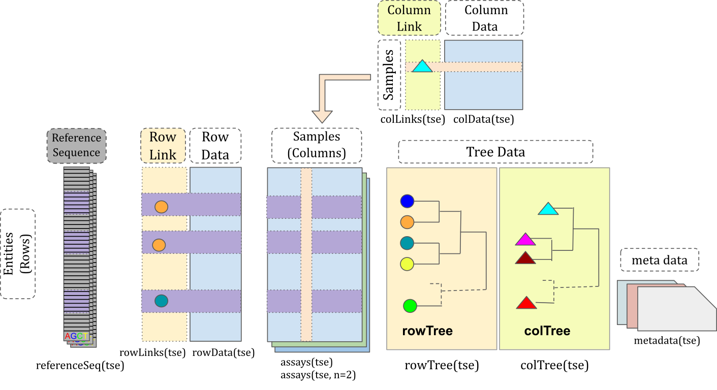
## miaverse (MIcrobiome Analysis) {width="50"}
- A framework for microbiome analytics
- [mia (analysis)](https://bioconductor.org/packages/release/bioc/html/mia.html)
- [miaViz (visualization)](https://bioconductor.org/packages/release/bioc/html/miaViz.html)
- [miaSim (simulation)](https://bioconductor.org/packages/release/bioc/html/miaSim.html)
- [Orchestrating Microbiome Analysis, OMA (tutorial book)](https://microbiome.github.io/OMA/)
- Based on *TreeSummarizedExperiment (TreeSE)* class
- Supports hierarchical data
- *phyloseq* class is a subset of *TreeSE*
- Extension of *SingleCellExperiment (SCE)* class
- miaverse is compatible with other *SummarizedExperiment* frameworks (especially [scater package](https://bioconductor.org/packages/release/bioc/html/scater.html))
- Purpose to offer tools and tips for microbiome data analysis
- Enables development of versatile analytical workflows in microbiome data science
- Supports multiomics (*MultiAssayExperiment* class)
- Scalable
- Standardized
{width="700"}
## The workflow
The workflow is based on [Orchestrating Microbiome Analysis (OMA) tutorial book](https://microbiome.github.io/OMA/).
Find more information from there.
### Importing the dataset
We fetch the data from [MGnify database](https://www.ebi.ac.uk/metagenomics).
It is a EMBL-EBI's database for metagenomic data. This large microbiome database
can be accessed with *MGnifyR* package which nowadays support *TreeSE*.
The package will be submitted to Bioconductor's next release.
We chose dataset of [study MGYS00005128](https://www.ebi.ac.uk/metagenomics/studies/MGYS00005128#overview).
In this study, they studied antibiotic resistance. They collected data from
Cambodia, Kenya and UK. The dataset contains total of 1197 samples with taxonomy
and gene function prediction data.
As loading takes some time, the dataset is already loaded.
```{r import1}
# library(MGnifyR)
# # Create a client object
# mg <- MgnifyClient(useCache = TRUE, cacheDir = "data/magnifyr_cache")
# # Search analysis IDs based on study ID
# analyses <- searchAnalysis(mg, "studies", "MGYS00005128")
# # Fetch data
# mae <- getResult(mg, analyses, get.func = "go-slim")
# # Store the data
# saveRDS(mae, "data/mae.Rds")
```
```{r import2}
mae <- readRDS("data/mae.Rds")
```
### The data containers
MAE stores multiple experiments, in this case 2 (taxonomy and gene function prediction info).
```{r data_container1}
mae
```
We can have general information on samples of the study in sample metadata of MAE.
```{r data_container2}
colData(mae)[1:5, 1:5] %>% kable()
```
MAE and TreeSE objects have rows and columns. This means that we can subset the
data similarly to other objects that have rows and columns (like data.frame).
In MAE, experiments and samples are linked together, meaning that we can subset
the data at one go.
For demonstrative purpose and for saving resources, let's subset the data by
taking 100 random samples.
```{r data_container3}
set.seed(49585)
random_samples <- sample(colnames(mae[[1]]), 100)
mae <- mae[, random_samples]
mae
```
The first experiment / TreeSE includes taxonomy information.
```{r data_container4}
mae[[1]]
```
The second one includes gene function prediction data. As you can see, we can
fetch the data by specifying index or name of experiment.
```{r data_container5}
mae[["go-slim"]]
```
Taxonomy information includes phylogenetic table in its feature metadata.
```{r data_container6}
rowData(mae[[1]]) %>% head() %>% kable()
```
Compared to phyloseq object, TreeSE can hold more data, for example, multiple
assays. Let's transform the data. Transformed table is stored to assays slot.
```{r data_container7}
mae[[1]] <- transformAssay(mae[[1]], method = "relabundance")
mae[[1]]
```
### Summarize data
We can summarize how many unique bacteria there in in certain taxonomy levels.
For instance, we can see that there are 53 unique bacterial phyla.
```{r summarize1}
rowData(mae[[1]]) %>% as_tibble() %>% summarise_all(n_distinct) %>% kable()
```
A common operation in microbiome data analysis is agglomeration. This means
that we sum-up the data to certain taxonomy levels. We can use
_mia::mergeFeaturesByRank_ function for agglomerating data to single
taxonomy level. If we want to agglomerate the data to all found taxonomy levels
with one command, we can use _mia::splitByRanks_.
altExp slot is the right place to store experiments with modified features
(such as agglomerated or subsetted data).
```{r summarize2}
altExps(mae[[1]]) <- splitByRanks(mae[[1]])
mae[[1]]
```
We can fetch agglomerated data from the slot. We can see that instead of 2207
features, there is only 5 features in the data that is summed-up to kingdom level.
```{r summarize3}
altExp(mae[[1]], "Kingdom")
```
assays include agglomerated abundance tables.
```{r summarize4}
assay(altExp(mae[[1]], "Kingdom"), "counts") %>% head() %>% kable()
```
To visualize phylogenetic relations, we can first create a phylogenetic tree
based on rowData, and then plot it. The tree is created in family level.
```{r summarize5}
altExp(mae[[1]], "Family") <- addTaxonomyTree(altExp(mae[[1]], "Family"))
plotRowTree(altExp(mae[[1]], "Family"), edge_colour_by = "Kingdom")
```
miaverse includes several visualizing methods. For example, we can visualize
relative abundances of 10 most abundant phyla.
```{r summarize6}
plotAbundanceDensity(
altExp(mae[[1]], "Phylum"), assay.type = "relabundance", n = 10, layout="density")
```
### Alpha diversity
Alpha diversity measures how diverse the microbial composition is. For example,
if there are lots of different bacterial species, the alpha diversity is higher.
Again, miaverse includes convenient tools to calculate alpha diversities of samples
and to visualize them.
Here we analyze if alpha diversities differ between locations.
```{r alpha}
# Calculate
mae[[1]] <- estimateDiversity(mae[[1]], index = "shannon")
# Plot
plotColData(mae[[1]], y = "shannon", x = "location", colour_by = "location") +
# These are normal ggplot objects
theme(legend.position = "none")
```
### Beta diversity
Beta diversity measures differences of microbial profiles of samples. There are
several techniques Principal Component Analysis (PCA) being the most well-known
ordination method. Distance-based redundancy analysis (dbRDA) is supervised
ordination method which takes into account sample metadata. It maximizes the
variance with respect to covariates.
Here we analyze if location can explain the differences in microbial profile.
The result is stored to reducedDim slot.
```{r beta1}
mae[[1]] <- runRDA(
mae[[1]],
assay.type = "relabundance",
formula = data ~ location,
distance = "bray",
name = "dbRDA"
)
reducedDim(mae[[1]], "dbRDA")
```
As we can see, location has significant effect on microbial profile. However,
from above we can see that groups do not have similar variance which is an
assumption of PERMANOVA. This has to be taken into account when making conclusions.
```{r beta2}
plotRDA(mae[[1]], "dbRDA", colour_by = "location")
```
### Differential abundance analysis (DAA)
The idea of DAA is to analyze, if there are bacteria whose abundance differ
between groups. There are multiple methods to test this (such as basic Wilcoxon test).
[ANCOM-BC](https://www.nature.com/articles/s41467-020-17041-7) is a method
that takes into consideration unique characters and features of microbial data.
Here we want to test if there are phyla whose abundance differ between locations.
```{r daa1}
# Analyze
res <- ancombc2(
data = altExp(mae[[1]], "Phylum"),
fix_formula = "location",
p_adj_method = "fdr",
group = "location",
global = TRUE
)
# Store results to data container
metadata( altExp(mae[[1]], "Phylum") )[["ancombc2"]] <- res
# Print
temp <- res$res_global
temp %>% kable()
```
```{r daa2}
# Add results to feature metadata
# Ensure that results go to right feature
rownames(temp) <- temp$taxon
temp <- temp[rownames(altExp(mae[[1]], "Phylum")), ]
rownames(temp) <- rownames( altExp(mae[[1]], "Phylum") )
# Add to rowData
rowData(altExp(mae[[1]], "Phylum")) <- cbind(rowData(altExp(mae[[1]], "Phylum")), temp)
```
We can visualize statistically significant features with boxplot.
```{r daa3, fig.width=12}
# Get the data from assay, rowData and colData
df <- meltAssay(altExp(mae[[1]], "Phylum"), assay.type = "relabundance", add_col_data = TRUE, add_row_data = TRUE)
# Take only significant features
df <- df[ df$diff_abn, ]
# Plot
ggplot(df, aes(x = location, colour = location, y = relabundance)) +
geom_boxplot(outlier.shape = NA) +
geom_jitter(width = 0.2) +
# Own panel for each feature
facet_grid(cols = vars(FeatureID)) +
# Remove x axis text
theme(axis.title.x=element_blank(), axis.text.x=element_blank()) +
# Logarithmic scale
scale_y_log10()
```
### Cross-correlation
To demonstrate, how we can integrate experiments, we perform simple cross-correlation
analysis. The purpose is to analyze, if there are phyla whose abundance correlates
with predicted gene functions.
First we subset the gene function prediction data by taking only those features
whose abundance varies the most across samples.
```{r crosscorr1}
# Transform assay
mae[[2]] <- transformAssay(mae[[2]], method = "log10", pseudocount = 1)
mae[[2]] <- transformAssay(mae[[2]], assay.type = "log10", method = "z", name = "log10_z")
# Get coefficients of variances
rowData(mae[[2]])[["cv"]] <- apply( assay(mae[[2]], "log10_z"), 1, function(x) sd(x)/mean(x) )
# Subset the data by taking top 40 features
top_feat <- order(abs(rowData(mae[[2]])[["cv"]]), decreasing = TRUE)[1:40]
altExp(mae[[2]], "sub") <- mae[[2]][top_feat, ]
# Replace feature names with more desriptive names
rownames(altExp(mae[[2]], "sub") ) <- rowData(altExp(mae[[2]], "sub"))[["description"]]
# Print
altExp(mae[[2]], "sub")
```
```{r crosscorr2, fig.width=13, fig.height=12}
# Transform assay of microbial data
altExp(mae[[1]], "Phylum") <- transformAssay(altExp(mae[[1]], "Phylum"), method = "clr", pseudocount = 1)
# Perform cross-correlation analysis
res <- testExperimentCrossAssociation(
mae,
experiment1 = 1, experiment2 = 2,
altexp1 = "Phylum", altexp2 = "sub",
assay.type1 = "clr", assay.type = "log10_z",
mode = "matrix"
)
# Store the result to data container
metadata(mae)[["croscor"]] <- res
# Plot
plot <- Heatmap(
res$cor, name = "Kendall's tau",
# Print values to cells
cell_fun = function(j, i, x, y, width, height, fill) {
# If the p-value is under threshold
if( !is.na(res$p_adj[i, j]) & res$p_adj[i, j] < 0.05 ){
# Print "X"
grid.text(sprintf("%s", "X"), x, y, gp = gpar(fontsize = 8, col = "black"))
}
},
column_names_rot = 45
)
# Adjust padding around plot so that names are visible
draw(plot, padding = unit(c(10, 40, 2, 2), "mm"))
```
### Save the results
Finally, we can save the data container which contains our analysis results.
```{r save}
saveRDS(mae, "data/mae_results.Rds")
```
## Thank you for your time!
- **Tuomas Borman -- doctoral researcher**
- Chouaib Benchraka -- doctoral researcher
- Leo Lahti -- group leader
------------------------------------------------------------------------
## Learning goals
1. Microbiome research studies interactions between microbes (and human, environment...)
2. Big data requires efficient tools to manipulate the data
3. miaverse is a (Tree)SummarizedExperiment framework for microbiome analytics
{width="400"}
## Motivation
### Microbiome research
- Microbiome is a composition of microbes in well-defined area (gut, skin, mouth...)
- Bilateral interaction between human and microbiome --> affects both health and disease.
- The research is based on sequencing (characterization of genes and species).
- Nowadays, multiomics approach is more common (integration of taxonomy information with metabolite data, for example)
- Computational methods are the new microscope
- The research has expanded rapidly in previous years
```{r pubmed_fig, fig.width=6, fig.cap="PubMed publications per year with a search term 'microbiome' (fetched: Sep 5, 2023)", class.source = 'fold-hide'}
# Plot publication graph
path <- "data/PubMed_Timeline_Results_by_Year.csv"
df <- read.csv(path, skip = 1)
x <- "Year"
y <- "Count"
plot <- ggplot(df, aes(x = .data[[x]], y = .data[[y]])) +
geom_bar(stat="identity")
plot
```
### Big data
- Cohort datasets are large in size
- Data management, handling and wrangling --\> data structure
- Computational power --\> High performance computing (HPC) and cloud computing
- [MultiAssayExperiment (MAE)](https://bioconductor.org/packages/release/bioc/html/MultiAssayExperiment.html) and [SummarizedExperiment (SE)](https://bioconductor.org/packages/release/bioc/html/SummarizedExperiment.html)
- Several R packages frameworks are increasingly integrating MAE and SE
- MAE enables linking of multiple experiments
- SE -- and especially TreeSE -- is an efficient data container to store data from an experiment
## miaverse (MIcrobiome Analysis) {width="50"}
- A framework for microbiome analytics
- [mia (analysis)](https://bioconductor.org/packages/release/bioc/html/mia.html)
- [miaViz (visualization)](https://bioconductor.org/packages/release/bioc/html/miaViz.html)
- [miaSim (simulation)](https://bioconductor.org/packages/release/bioc/html/miaSim.html)
- [Orchestrating Microbiome Analysis, OMA (tutorial book)](https://microbiome.github.io/OMA/)
- Based on *TreeSummarizedExperiment (TreeSE)* class
- Supports hierarchical data
- *phyloseq* class is a subset of *TreeSE*
- Extension of *SingleCellExperiment (SCE)* class
- miaverse is compatible with other *SummarizedExperiment* frameworks (especially [scater package](https://bioconductor.org/packages/release/bioc/html/scater.html))
- Purpose to offer tools and tips for microbiome data analysis
- Enables development of versatile analytical workflows in microbiome data science
- Supports multiomics (*MultiAssayExperiment* class)
- Scalable
- Standardized
{width="700"}
## The workflow
The workflow is based on [Orchestrating Microbiome Analysis (OMA) tutorial book](https://microbiome.github.io/OMA/).
Find more information from there.
### Importing the dataset
We fetch the data from [MGnify database](https://www.ebi.ac.uk/metagenomics).
It is a EMBL-EBI's database for metagenomic data. This large microbiome database
can be accessed with *MGnifyR* package which nowadays support *TreeSE*.
The package will be submitted to Bioconductor's next release.
We chose dataset of [study MGYS00005128](https://www.ebi.ac.uk/metagenomics/studies/MGYS00005128#overview).
In this study, they studied antibiotic resistance. They collected data from
Cambodia, Kenya and UK. The dataset contains total of 1197 samples with taxonomy
and gene function prediction data.
As loading takes some time, the dataset is already loaded.
```{r import1}
# library(MGnifyR)
# # Create a client object
# mg <- MgnifyClient(useCache = TRUE, cacheDir = "data/magnifyr_cache")
# # Search analysis IDs based on study ID
# analyses <- searchAnalysis(mg, "studies", "MGYS00005128")
# # Fetch data
# mae <- getResult(mg, analyses, get.func = "go-slim")
# # Store the data
# saveRDS(mae, "data/mae.Rds")
```
```{r import2}
mae <- readRDS("data/mae.Rds")
```
### The data containers
MAE stores multiple experiments, in this case 2 (taxonomy and gene function prediction info).
```{r data_container1}
mae
```
We can have general information on samples of the study in sample metadata of MAE.
```{r data_container2}
colData(mae)[1:5, 1:5] %>% kable()
```
MAE and TreeSE objects have rows and columns. This means that we can subset the
data similarly to other objects that have rows and columns (like data.frame).
In MAE, experiments and samples are linked together, meaning that we can subset
the data at one go.
For demonstrative purpose and for saving resources, let's subset the data by
taking 100 random samples.
```{r data_container3}
set.seed(49585)
random_samples <- sample(colnames(mae[[1]]), 100)
mae <- mae[, random_samples]
mae
```
The first experiment / TreeSE includes taxonomy information.
```{r data_container4}
mae[[1]]
```
The second one includes gene function prediction data. As you can see, we can
fetch the data by specifying index or name of experiment.
```{r data_container5}
mae[["go-slim"]]
```
Taxonomy information includes phylogenetic table in its feature metadata.
```{r data_container6}
rowData(mae[[1]]) %>% head() %>% kable()
```
Compared to phyloseq object, TreeSE can hold more data, for example, multiple
assays. Let's transform the data. Transformed table is stored to assays slot.
```{r data_container7}
mae[[1]] <- transformAssay(mae[[1]], method = "relabundance")
mae[[1]]
```
### Summarize data
We can summarize how many unique bacteria there in in certain taxonomy levels.
For instance, we can see that there are 53 unique bacterial phyla.
```{r summarize1}
rowData(mae[[1]]) %>% as_tibble() %>% summarise_all(n_distinct) %>% kable()
```
A common operation in microbiome data analysis is agglomeration. This means
that we sum-up the data to certain taxonomy levels. We can use
_mia::mergeFeaturesByRank_ function for agglomerating data to single
taxonomy level. If we want to agglomerate the data to all found taxonomy levels
with one command, we can use _mia::splitByRanks_.
altExp slot is the right place to store experiments with modified features
(such as agglomerated or subsetted data).
```{r summarize2}
altExps(mae[[1]]) <- splitByRanks(mae[[1]])
mae[[1]]
```
We can fetch agglomerated data from the slot. We can see that instead of 2207
features, there is only 5 features in the data that is summed-up to kingdom level.
```{r summarize3}
altExp(mae[[1]], "Kingdom")
```
assays include agglomerated abundance tables.
```{r summarize4}
assay(altExp(mae[[1]], "Kingdom"), "counts") %>% head() %>% kable()
```
To visualize phylogenetic relations, we can first create a phylogenetic tree
based on rowData, and then plot it. The tree is created in family level.
```{r summarize5}
altExp(mae[[1]], "Family") <- addTaxonomyTree(altExp(mae[[1]], "Family"))
plotRowTree(altExp(mae[[1]], "Family"), edge_colour_by = "Kingdom")
```
miaverse includes several visualizing methods. For example, we can visualize
relative abundances of 10 most abundant phyla.
```{r summarize6}
plotAbundanceDensity(
altExp(mae[[1]], "Phylum"), assay.type = "relabundance", n = 10, layout="density")
```
### Alpha diversity
Alpha diversity measures how diverse the microbial composition is. For example,
if there are lots of different bacterial species, the alpha diversity is higher.
Again, miaverse includes convenient tools to calculate alpha diversities of samples
and to visualize them.
Here we analyze if alpha diversities differ between locations.
```{r alpha}
# Calculate
mae[[1]] <- estimateDiversity(mae[[1]], index = "shannon")
# Plot
plotColData(mae[[1]], y = "shannon", x = "location", colour_by = "location") +
# These are normal ggplot objects
theme(legend.position = "none")
```
### Beta diversity
Beta diversity measures differences of microbial profiles of samples. There are
several techniques Principal Component Analysis (PCA) being the most well-known
ordination method. Distance-based redundancy analysis (dbRDA) is supervised
ordination method which takes into account sample metadata. It maximizes the
variance with respect to covariates.
Here we analyze if location can explain the differences in microbial profile.
The result is stored to reducedDim slot.
```{r beta1}
mae[[1]] <- runRDA(
mae[[1]],
assay.type = "relabundance",
formula = data ~ location,
distance = "bray",
name = "dbRDA"
)
reducedDim(mae[[1]], "dbRDA")
```
As we can see, location has significant effect on microbial profile. However,
from above we can see that groups do not have similar variance which is an
assumption of PERMANOVA. This has to be taken into account when making conclusions.
```{r beta2}
plotRDA(mae[[1]], "dbRDA", colour_by = "location")
```
### Differential abundance analysis (DAA)
The idea of DAA is to analyze, if there are bacteria whose abundance differ
between groups. There are multiple methods to test this (such as basic Wilcoxon test).
[ANCOM-BC](https://www.nature.com/articles/s41467-020-17041-7) is a method
that takes into consideration unique characters and features of microbial data.
Here we want to test if there are phyla whose abundance differ between locations.
```{r daa1}
# Analyze
res <- ancombc2(
data = altExp(mae[[1]], "Phylum"),
fix_formula = "location",
p_adj_method = "fdr",
group = "location",
global = TRUE
)
# Store results to data container
metadata( altExp(mae[[1]], "Phylum") )[["ancombc2"]] <- res
# Print
temp <- res$res_global
temp %>% kable()
```
```{r daa2}
# Add results to feature metadata
# Ensure that results go to right feature
rownames(temp) <- temp$taxon
temp <- temp[rownames(altExp(mae[[1]], "Phylum")), ]
rownames(temp) <- rownames( altExp(mae[[1]], "Phylum") )
# Add to rowData
rowData(altExp(mae[[1]], "Phylum")) <- cbind(rowData(altExp(mae[[1]], "Phylum")), temp)
```
We can visualize statistically significant features with boxplot.
```{r daa3, fig.width=12}
# Get the data from assay, rowData and colData
df <- meltAssay(altExp(mae[[1]], "Phylum"), assay.type = "relabundance", add_col_data = TRUE, add_row_data = TRUE)
# Take only significant features
df <- df[ df$diff_abn, ]
# Plot
ggplot(df, aes(x = location, colour = location, y = relabundance)) +
geom_boxplot(outlier.shape = NA) +
geom_jitter(width = 0.2) +
# Own panel for each feature
facet_grid(cols = vars(FeatureID)) +
# Remove x axis text
theme(axis.title.x=element_blank(), axis.text.x=element_blank()) +
# Logarithmic scale
scale_y_log10()
```
### Cross-correlation
To demonstrate, how we can integrate experiments, we perform simple cross-correlation
analysis. The purpose is to analyze, if there are phyla whose abundance correlates
with predicted gene functions.
First we subset the gene function prediction data by taking only those features
whose abundance varies the most across samples.
```{r crosscorr1}
# Transform assay
mae[[2]] <- transformAssay(mae[[2]], method = "log10", pseudocount = 1)
mae[[2]] <- transformAssay(mae[[2]], assay.type = "log10", method = "z", name = "log10_z")
# Get coefficients of variances
rowData(mae[[2]])[["cv"]] <- apply( assay(mae[[2]], "log10_z"), 1, function(x) sd(x)/mean(x) )
# Subset the data by taking top 40 features
top_feat <- order(abs(rowData(mae[[2]])[["cv"]]), decreasing = TRUE)[1:40]
altExp(mae[[2]], "sub") <- mae[[2]][top_feat, ]
# Replace feature names with more desriptive names
rownames(altExp(mae[[2]], "sub") ) <- rowData(altExp(mae[[2]], "sub"))[["description"]]
# Print
altExp(mae[[2]], "sub")
```
```{r crosscorr2, fig.width=13, fig.height=12}
# Transform assay of microbial data
altExp(mae[[1]], "Phylum") <- transformAssay(altExp(mae[[1]], "Phylum"), method = "clr", pseudocount = 1)
# Perform cross-correlation analysis
res <- testExperimentCrossAssociation(
mae,
experiment1 = 1, experiment2 = 2,
altexp1 = "Phylum", altexp2 = "sub",
assay.type1 = "clr", assay.type = "log10_z",
mode = "matrix"
)
# Store the result to data container
metadata(mae)[["croscor"]] <- res
# Plot
plot <- Heatmap(
res$cor, name = "Kendall's tau",
# Print values to cells
cell_fun = function(j, i, x, y, width, height, fill) {
# If the p-value is under threshold
if( !is.na(res$p_adj[i, j]) & res$p_adj[i, j] < 0.05 ){
# Print "X"
grid.text(sprintf("%s", "X"), x, y, gp = gpar(fontsize = 8, col = "black"))
}
},
column_names_rot = 45
)
# Adjust padding around plot so that names are visible
draw(plot, padding = unit(c(10, 40, 2, 2), "mm"))
```
### Save the results
Finally, we can save the data container which contains our analysis results.
```{r save}
saveRDS(mae, "data/mae_results.Rds")
```
## Thank you for your time!
 ### Key points
1. Microbiome research studies interactions between microbes (and human, environment...)
2. Big data requires efficient tools to manipulate the data
3. miaverse is a (Tree)SummarizedExperiment framework for microbiome analytics
### More information
- [Project website](https://microbiome.github.io/)
- Poster: miaverse -- microbiome analytics framework in SummarizedExperiment family
## Session info
```{r sessioninfo, class.source = 'fold-hide'}
sessionInfo()
```
### Key points
1. Microbiome research studies interactions between microbes (and human, environment...)
2. Big data requires efficient tools to manipulate the data
3. miaverse is a (Tree)SummarizedExperiment framework for microbiome analytics
### More information
- [Project website](https://microbiome.github.io/)
- Poster: miaverse -- microbiome analytics framework in SummarizedExperiment family
## Session info
```{r sessioninfo, class.source = 'fold-hide'}
sessionInfo()
```