balance command
Syntax
balance thresh style args ... keyword value ...
- thresh = imbalance threshhold that must be exceeded to perform a re-balance
- one style/arg pair can be used (or multiple for x,*y*,*z*)
- style = x or y or z or shift or rcb
x args = uniform or Px-1 numbers between 0 and 1
  uniform = evenly spaced cuts between processors in x dimension
  numbers = Px-1 ascending values between 0 and 1, Px - # of processors in x dimension
  x can be specified together with y or z
y args = uniform or Py-1 numbers between 0 and 1
  uniform = evenly spaced cuts between processors in y dimension
  numbers = Py-1 ascending values between 0 and 1, Py - # of processors in y dimension
  y can be specified together with x or z
z args = uniform or Pz-1 numbers between 0 and 1
  uniform = evenly spaced cuts between processors in z dimension
  numbers = Pz-1 ascending values between 0 and 1, Pz - # of processors in z dimension
  z can be specified together with x or y
shift args = dimstr Niter stopthresh
  dimstr = sequence of letters containing "x" or "y" or "z", each not more than once
  Niter = # of times to iterate within each dimension of dimstr sequence
  stopthresh = stop balancing when this imbalance threshhold is reached
rcb args = none
- zero or more keyword/value pairs may be appended
- keyword = out
out value = filename
  filename = write each processor's sub-domain to a file
Examples
balance 0.9 x uniform y 0.4 0.5 0.6
balance 1.2 shift xz 5 1.1
balance 1.0 shift xz 5 1.1
balance 1.1 rcb
balance 1.0 shift x 20 1.0 out tmp.balance
Description
This command adjusts the size and shape of processor sub-domains within the simulation box, to attempt to balance the number of particles and thus the computational cost (load) evenly across processors. The load balancing is “static” in the sense that this command performs the balancing once, before or between simulations. The processor sub-domains will then remain static during the subsequent run. To perform “dynamic” balancing, see the fix balance command, which can adjust processor sub-domain sizes and shapes on-the-fly during a run.
Load-balancing is typically only useful if the particles in the simulation box have a spatially-varying density distribution. E.g. a model of a vapor/liquid interface, or a solid with an irregular-shaped geometry containing void regions. In this case, the LAMMPS default of dividing the simulation box volume into a regular-spaced grid of 3d bricks, with one equal-volume sub-domain per procesor, may assign very different numbers of particles per processor. This can lead to poor performance when the simulation is run in parallel.
Note that the processors command allows some control over how the box volume is split across processors. Specifically, for a Px by Py by Pz grid of processors, it allows choice of Px, Py, and Pz, subject to the constraint that Px * Py * Pz = P, the total number of processors. This is sufficient to achieve good load-balance for some problems on some processor counts. However, all the processor sub-domains will still have the same shape and same volume.
The requested load-balancing operation is only performed if the current “imbalance factor” in particles owned by each processor exceeds the specified thresh parameter. The imbalance factor is defined as the maximum number of particles owned by any processor, divided by the average number of particles per processor. Thus an imbalance factor of 1.0 is perfect balance.
As an example, for 10000 particles running on 10 processors, if the most heavily loaded processor has 1200 particles, then the factor is 1.2, meaning there is a 20% imbalance. Note that a re-balance can be forced even if the current balance is perfect (1.0) be specifying a thresh < 1.0.
Note
Balancing is performed even if the imbalance factor does not exceed the thresh parameter if a “grid” style is specified when the current partitioning is “tiled”. The meaning of “grid” vs “tiled” is explained below. This is to allow forcing of the partitioning to “grid” so that the comm_style brick command can then be used to replace a current comm_style tiled setting.
When the balance command completes, it prints statistics about the result, including the change in the imbalance factor and the change in the maximum number of particles on any processor. For “grid” methods (defined below) that create a logical 3d grid of processors, the positions of all cutting planes in each of the 3 dimensions (as fractions of the box length) are also printed.
Note
This command attempts to minimize the imbalance factor, as defined above. But depending on the method a perfect balance (1.0) may not be achieved. For example, “grid” methods (defined below) that create a logical 3d grid cannot achieve perfect balance for many irregular distributions of particles. Likewise, if a portion of the system is a perfect lattice, e.g. the intiial system is generated by the create_atoms command, then “grid” methods may be unable to achieve exact balance. This is because entire lattice planes will be owned or not owned by a single processor.
Note
The imbalance factor is also an estimate of the maximum speed-up you can hope to achieve by running a perfectly balanced simulation versus an imbalanced one. In the example above, the 10000 particle simulation could run up to 20% faster if it were perfectly balanced, versus when imbalanced. However, computational cost is not strictly proportional to particle count, and changing the relative size and shape of processor sub-domains may lead to additional computational and communication overheads, e.g. in the PPPM solver used via the kspace_style command. Thus you should benchmark the run times of a simulation before and after balancing.
The method used to perform a load balance is specified by one of the listed styles (or more in the case of x,*y*,*z*), which are described in detail below. There are 2 kinds of styles.
The x, y, z, and shift styles are “grid” methods which produce a logical 3d grid of processors. They operate by changing the cutting planes (or lines) between processors in 3d (or 2d), to adjust the volume (area in 2d) assigned to each processor, as in the following 2d diagram where processor sub-domains are shown and atoms are colored by the processor that owns them. The leftmost diagram is the default partitioning of the simulation box across processors (one sub-box for each of 16 processors); the middle diagram is after a “grid” method has been applied.
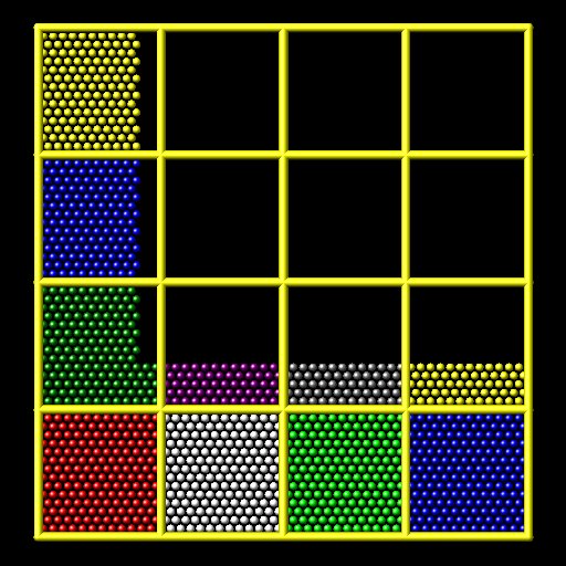
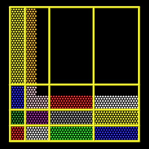
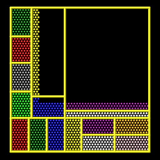
The rcb style is a “tiling” method which does not produce a logical 3d grid of processors. Rather it tiles the simulation domain with rectangular sub-boxes of varying size and shape in an irregular fashion so as to have equal numbers of particles in each sub-box, as in the rightmost diagram above.
The “grid” methods can be used with either of the comm_style command options, brick or tiled. The “tiling” methods can only be used with comm_style tiled. Note that it can be useful to use a “grid” method with comm_style tiled to return the domain partitioning to a logical 3d grid of processors so that “comm_style brick” can afterwords be specified for subsequent run commands.
When a “grid” method is specified, the current domain partitioning can be either a logical 3d grid or a tiled partitioning. In the former case, the current logical 3d grid is used as a starting point and changes are made to improve the imbalance factor. In the latter case, the tiled partitioning is discarded and a logical 3d grid is created with uniform spacing in all dimensions. This becomes the starting point for the balancing operation.
When a “tiling” method is specified, the current domain partitioning (“grid” or “tiled”) is ignored, and a new partitioning is computed from scratch.
The x, y, and z styles invoke a “grid” method for balancing, as described above. Note that any or all of these 3 styles can be specified together, one after the other, but they cannot be used with any other style. This style adjusts the position of cutting planes between processor sub-domains in specific dimensions. Only the specified dimensions are altered.
The uniform argument spaces the planes evenly, as in the left diagrams above. The numeric argument requires listing Ps-1 numbers that specify the position of the cutting planes. This requires knowing Ps = Px or Py or Pz = the number of processors assigned by LAMMPS to the relevant dimension. This assignment is made (and the Px, Py, Pz values printed out) when the simulation box is created by the “create_box” or “read_data” or “read_restart” command and is influenced by the settings of the processors command.
Each of the numeric values must be between 0 and 1, and they must be listed in ascending order. They represent the fractional position of the cutting place. The left (or lower) edge of the box is 0.0, and the right (or upper) edge is 1.0. Neither of these values is specified. Only the interior Ps-1 positions are specified. Thus is there are 2 procesors in the x dimension, you specify a single value such as 0.75, which would make the left processor’s sub-domain 3x larger than the right processor’s sub-domain.
The shift style invokes a “grid” method for balancing, as described above. It changes the positions of cutting planes between processors in an iterative fashion, seeking to reduce the imbalance factor, similar to how the fix balance shift command operates.
The dimstr argument is a string of characters, each of which must be an “x” or “y” or “z”. Eacn character can appear zero or one time, since there is no advantage to balancing on a dimension more than once. You should normally only list dimensions where you expect there to be a density variation in the particles.
Balancing proceeds by adjusting the cutting planes in each of the dimensions listed in dimstr, one dimension at a time. For a single dimension, the balancing operation (described below) is iterated on up to Niter times. After each dimension finishes, the imbalance factor is re-computed, and the balancing operation halts if the stopthresh criterion is met.
A rebalance operation in a single dimension is performed using a recursive multisectioning algorithm, where the position of each cutting plane (line in 2d) in the dimension is adjusted independently. This is similar to a recursive bisectioning for a single value, except that the bounds used for each bisectioning take advantage of information from neighboring cuts if possible. At each iteration, the count of particles on either side of each plane is tallied. If the counts do not match the target value for the plane, the position of the cut is adjusted to be halfway between a low and high bound. The low and high bounds are adjusted on each iteration, using new count information, so that they become closer together over time. Thus as the recustion progresses, the count of particles on either side of the plane gets closer to the target value.
Once the rebalancing is complete and final processor sub-domains assigned, particles are migrated to their new owning processor, and the balance procedure ends.
Note
At each rebalance operation, the bisectioning for each cutting plane (line in 2d) typcially starts with low and high bounds separated by the extent of a processor’s sub-domain in one dimension. The size of this bracketing region shrinks by 1/2 every iteration. Thus if Niter is specified as 10, the cutting plane will typically be positioned to 1 part in 1000 accuracy (relative to the perfect target position). For Niter = 20, it will be accurate to 1 part in a million. Thus there is no need ot set Niter to a large value. LAMMPS will check if the threshold accuracy is reached (in a dimension) is less iterations than Niter and exit early. However, Niter should also not be set too small, since it will take roughly the same number of iterations to converge even if the cutting plane is initially close to the target value.
The rcb style invokes a “tiled” method for balancing, as described above. It performs a recursive coordinate bisectioning (RCB) of the simulation domain. The basic idea is as follows.
The simulation domain is cut into 2 boxes by an axis-aligned cut in the longest dimension, leaving one new box on either side of the cut. All the processors are also partitioned into 2 groups, half assigned to the box on the lower side of the cut, and half to the box on the upper side. (If the processor count is odd, one side gets an extra processor.) The cut is positioned so that the number of atoms in the lower box is exactly the number that the processors assigned to that box should own for load balance to be perfect. This also makes load balance for the upper box perfect. The positioning is done iteratively, by a bisectioning method. Note that counting atoms on either side of the cut requires communication between all processors at each iteration.
That is the procedure for the first cut. Subsequent cuts are made recursively, in exactly the same manner. The subset of processors assigned to each box make a new cut in the longest dimension of that box, splitting the box, the subset of processsors, and the atoms in the box in two. The recursion continues until every processor is assigned a sub-box of the entire simulation domain, and owns the atoms in that sub-box.
The out keyword writes a text file to the specified filename with the results of the balancing operation. The file contains the bounds of the sub-domain for each processor after the balancing operation completes. The format of the file is compatible with the Pizza.py mdump tool which has support for manipulating and visualizing mesh files. An example is shown here for a balancing by 4 processors for a 2d problem:
ITEM: TIMESTEP
0
ITEM: NUMBER OF NODES
16
ITEM: BOX BOUNDS
0 10
0 10
0 10
ITEM: NODES
1 1 0 0 0
2 1 5 0 0
3 1 5 5 0
4 1 0 5 0
5 1 5 0 0
6 1 10 0 0
7 1 10 5 0
8 1 5 5 0
9 1 0 5 0
10 1 5 5 0
11 1 5 10 0
12 1 10 5 0
13 1 5 5 0
14 1 10 5 0
15 1 10 10 0
16 1 5 10 0
ITEM: TIMESTEP
0
ITEM: NUMBER OF SQUARES
4
ITEM: SQUARES
1 1 1 2 3 4
2 1 5 6 7 8
3 1 9 10 11 12
4 1 13 14 15 16
The coordinates of all the vertices are listed in the NODES section, 5 per processor. Note that the 4 sub-domains share vertices, so there will be duplicate nodes in the list.
The “SQUARES” section lists the node IDs of the 4 vertices in a rectangle for each processor (1 to 4).
For a 3d problem, the syntax is similar with 8 vertices listed for each processor, instead of 4, and “SQUARES” replaced by “CUBES”.
Restrictions
For 2d simulations, the z style cannot be used. Nor can a “z” appear in dimstr for the shift style.