 \n",
"\n",
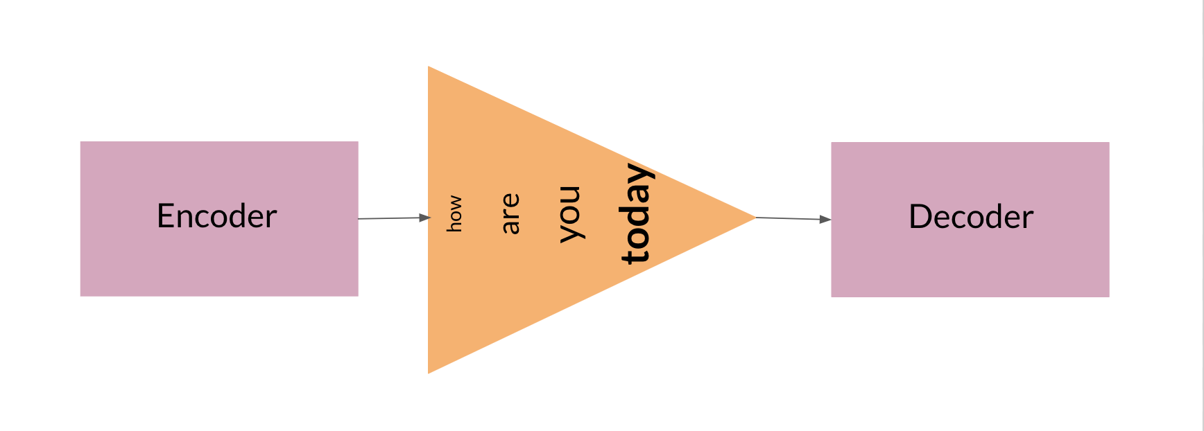
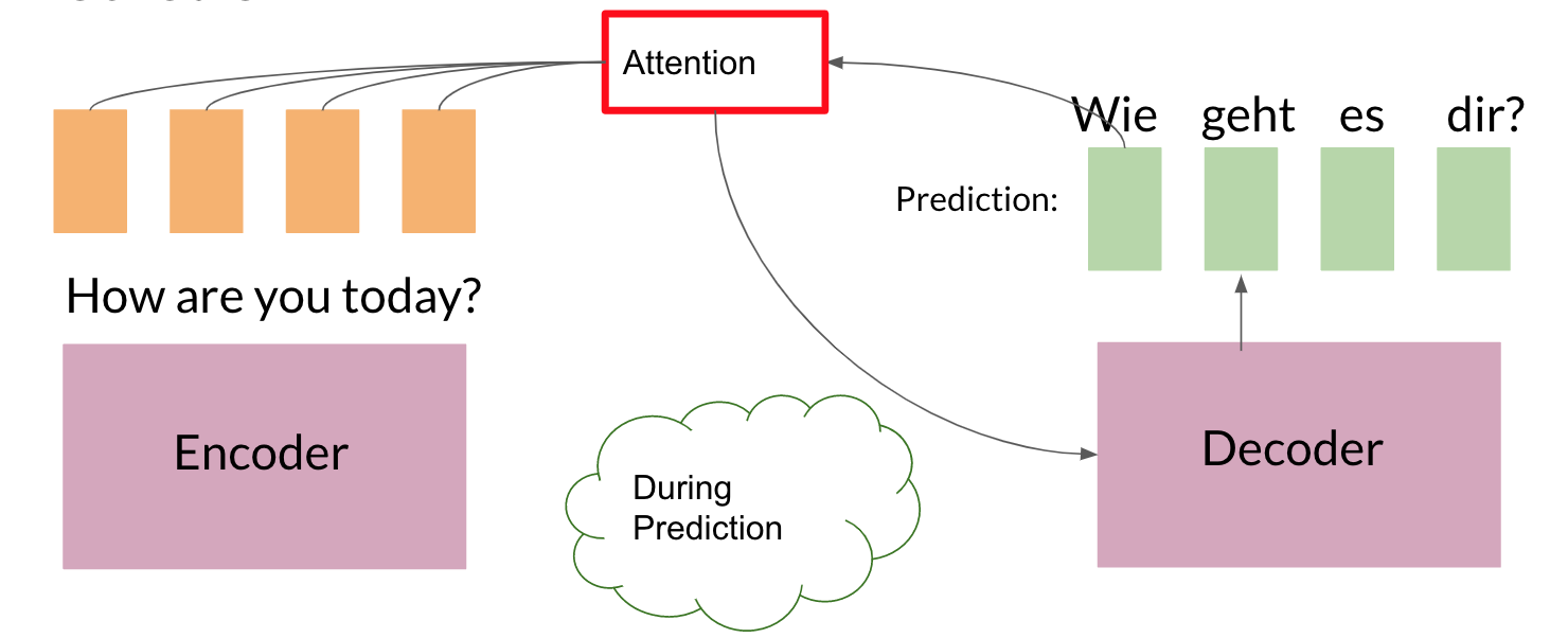
"Adding an attention layer to this model avoids this problem by giving the decoder access to all parts of the input sentence. To illustrate, let's just use a 4-word input sentence as shown below. Remember that a hidden state is produced at each timestep of the encoder (represented by the orange rectangles). These are all passed to the attention layer and each are given a score given the current activation (i.e. hidden state) of the decoder. For instance, let's consider the figure below where the first prediction \"Wie\" is already made. To produce the next prediction, the attention layer will first receive all the encoder hidden states (i.e. orange rectangles) as well as the decoder hidden state when producing the word \"Wie\" (i.e. first green rectangle). Given these information, it will score each of the encoder hidden states to know which one the decoder should focus on to produce the next word. The result of the model training might have learned that it should align to the second encoder hidden state and subsequently assigns a high probability to the word \"geht\". If we are using greedy decoding, we will output the said word as the next symbol, then restart the process to produce the next word until we reach an end-of-sentence prediction.\n",
"\n",
"
\n",
"\n",
"Adding an attention layer to this model avoids this problem by giving the decoder access to all parts of the input sentence. To illustrate, let's just use a 4-word input sentence as shown below. Remember that a hidden state is produced at each timestep of the encoder (represented by the orange rectangles). These are all passed to the attention layer and each are given a score given the current activation (i.e. hidden state) of the decoder. For instance, let's consider the figure below where the first prediction \"Wie\" is already made. To produce the next prediction, the attention layer will first receive all the encoder hidden states (i.e. orange rectangles) as well as the decoder hidden state when producing the word \"Wie\" (i.e. first green rectangle). Given these information, it will score each of the encoder hidden states to know which one the decoder should focus on to produce the next word. The result of the model training might have learned that it should align to the second encoder hidden state and subsequently assigns a high probability to the word \"geht\". If we are using greedy decoding, we will output the said word as the next symbol, then restart the process to produce the next word until we reach an end-of-sentence prediction.\n",
"\n",
" \n",
"\n",
"\n",
"There are different ways to implement attention and the one we'll use for this assignment is the Scaled Dot Product Attention which has the form:\n",
"\n",
"$$Attention(Q, K, V) = softmax(\\frac{QK^T}{\\sqrt{d_k}})V$$\n",
"\n",
"You will dive deeper into this equation in the next week but for now, you can think of it as computing scores using queries (Q) and keys (K), followed by a multiplication of values (V) to get a context vector at a particular timestep of the decoder. This context vector is fed to the decoder RNN to get a set of probabilities for the next predicted word. The division by square root of the keys dimensionality ($\\sqrt{d_k}$) is for improving model performance and you'll also learn more about it next week. For our machine translation application, the encoder activations (i.e. encoder hidden states) will be the keys and values, while the decoder activations (i.e. decoder hidden states) will be the queries.\n",
"\n",
"You will see in the upcoming sections that this complex architecture and mechanism can be implemented with just a few lines of code. Let's get started!"
]
},
{
"cell_type": "markdown",
"metadata": {},
"source": [
"\n",
"## 2.2 Helper functions\n",
"\n",
"We will first implement a few functions that we will use later on. These will be for the input encoder, pre-attention decoder, and preparation of the queries, keys, values, and mask.\n",
"\n",
"### 2.2.1 Input encoder\n",
"\n",
"The input encoder runs on the input tokens, creates its embeddings, and feeds it to an LSTM network. This outputs the activations that will be the keys and values for attention. It is a [Serial](https://trax-ml.readthedocs.io/en/latest/trax.layers.html#trax.layers.combinators.Serial) network which uses:\n",
"\n",
" - [tl.Embedding](https://trax-ml.readthedocs.io/en/latest/trax.layers.html#trax.layers.core.Embedding): Converts each token to its vector representation. In this case, it is the the size of the vocabulary by the dimension of the model: `tl.Embedding(vocab_size, d_model)`. `vocab_size` is the number of entries in the given vocabulary. `d_model` is the number of elements in the word embedding.\n",
" \n",
" - [tl.LSTM](https://trax-ml.readthedocs.io/en/latest/trax.layers.html#trax.layers.rnn.LSTM): LSTM layer of size `d_model`. We want to be able to configure how many encoder layers we have so remember to create LSTM layers equal to the number of the `n_encoder_layers` parameter.\n",
" \n",
"
\n",
"\n",
"\n",
"There are different ways to implement attention and the one we'll use for this assignment is the Scaled Dot Product Attention which has the form:\n",
"\n",
"$$Attention(Q, K, V) = softmax(\\frac{QK^T}{\\sqrt{d_k}})V$$\n",
"\n",
"You will dive deeper into this equation in the next week but for now, you can think of it as computing scores using queries (Q) and keys (K), followed by a multiplication of values (V) to get a context vector at a particular timestep of the decoder. This context vector is fed to the decoder RNN to get a set of probabilities for the next predicted word. The division by square root of the keys dimensionality ($\\sqrt{d_k}$) is for improving model performance and you'll also learn more about it next week. For our machine translation application, the encoder activations (i.e. encoder hidden states) will be the keys and values, while the decoder activations (i.e. decoder hidden states) will be the queries.\n",
"\n",
"You will see in the upcoming sections that this complex architecture and mechanism can be implemented with just a few lines of code. Let's get started!"
]
},
{
"cell_type": "markdown",
"metadata": {},
"source": [
"\n",
"## 2.2 Helper functions\n",
"\n",
"We will first implement a few functions that we will use later on. These will be for the input encoder, pre-attention decoder, and preparation of the queries, keys, values, and mask.\n",
"\n",
"### 2.2.1 Input encoder\n",
"\n",
"The input encoder runs on the input tokens, creates its embeddings, and feeds it to an LSTM network. This outputs the activations that will be the keys and values for attention. It is a [Serial](https://trax-ml.readthedocs.io/en/latest/trax.layers.html#trax.layers.combinators.Serial) network which uses:\n",
"\n",
" - [tl.Embedding](https://trax-ml.readthedocs.io/en/latest/trax.layers.html#trax.layers.core.Embedding): Converts each token to its vector representation. In this case, it is the the size of the vocabulary by the dimension of the model: `tl.Embedding(vocab_size, d_model)`. `vocab_size` is the number of entries in the given vocabulary. `d_model` is the number of elements in the word embedding.\n",
" \n",
" - [tl.LSTM](https://trax-ml.readthedocs.io/en/latest/trax.layers.html#trax.layers.rnn.LSTM): LSTM layer of size `d_model`. We want to be able to configure how many encoder layers we have so remember to create LSTM layers equal to the number of the `n_encoder_layers` parameter.\n",
" \n",
" \n",
"\n",
"\n",
"### Exercise 01\n",
"\n",
"**Instructions:** Implement the `input_encoder_fn` function."
]
},
{
"cell_type": "code",
"execution_count": 12,
"metadata": {},
"outputs": [],
"source": [
"# UNQ_C1\n",
"# GRADED FUNCTION\n",
"def input_encoder_fn(input_vocab_size, d_model, n_encoder_layers):\n",
" \"\"\" Input encoder runs on the input sentence and creates\n",
" activations that will be the keys and values for attention.\n",
" \n",
" Args:\n",
" input_vocab_size: int: vocab size of the input\n",
" d_model: int: depth of embedding (n_units in the LSTM cell)\n",
" n_encoder_layers: int: number of LSTM layers in the encoder\n",
" Returns:\n",
" tl.Serial: The input encoder\n",
" \"\"\"\n",
" \n",
" # create a serial network\n",
" input_encoder = tl.Serial( \n",
" \n",
" ### START CODE HERE (REPLACE INSTANCES OF `None` WITH YOUR CODE) ###\n",
" # create an embedding layer to convert tokens to vectors\n",
" tl.Embedding(vocab_size=input_vocab_size, d_feature=d_model),\n",
" \n",
" # feed the embeddings to the LSTM layers. It is a stack of n_encoder_layers LSTM layers\n",
" [tl.LSTM(n_units=d_model) for _ in range(n_encoder_layers)]\n",
" ### END CODE HERE ###\n",
" )\n",
"\n",
" return input_encoder"
]
},
{
"cell_type": "markdown",
"metadata": {},
"source": [
"*Note: To make this notebook more neat, we moved the unit tests to a separate file called `w1_unittest.py`. Feel free to open it from your workspace if needed. We have placed comments in that file to indicate which functions are testing which part of the assignment (e.g. `test_input_encoder_fn()` has the unit tests for UNQ_C1).*"
]
},
{
"cell_type": "code",
"execution_count": 13,
"metadata": {},
"outputs": [
{
"name": "stdout",
"output_type": "stream",
"text": [
"\u001b[92m All tests passed\n"
]
}
],
"source": [
"# BEGIN UNIT TEST\n",
"import w1_unittest\n",
"\n",
"w1_unittest.test_input_encoder_fn(input_encoder_fn)\n",
"# END UNIT TEST"
]
},
{
"cell_type": "markdown",
"metadata": {},
"source": [
"### 2.2.2 Pre-attention decoder\n",
"\n",
"The pre-attention decoder runs on the targets and creates activations that are used as queries in attention. This is a Serial network which is composed of the following:\n",
"\n",
" - [tl.ShiftRight](https://trax-ml.readthedocs.io/en/latest/trax.layers.html#trax.layers.attention.ShiftRight): This pads a token to the beginning of your target tokens (e.g. `[8, 34, 12]` shifted right is `[0, 8, 34, 12]`). This will act like a start-of-sentence token that will be the first input to the decoder. During training, this shift also allows the target tokens to be passed as input to do teacher forcing.\n",
"\n",
" - [tl.Embedding](https://trax-ml.readthedocs.io/en/latest/trax.layers.html#trax.layers.core.Embedding): Like in the previous function, this converts each token to its vector representation. In this case, it is the the size of the vocabulary by the dimension of the model: `tl.Embedding(vocab_size, d_model)`. `vocab_size` is the number of entries in the given vocabulary. `d_model` is the number of elements in the word embedding.\n",
" \n",
" - [tl.LSTM](https://trax-ml.readthedocs.io/en/latest/trax.layers.html#trax.layers.rnn.LSTM): LSTM layer of size `d_model`.\n",
"\n",
"
\n",
"\n",
"\n",
"### Exercise 01\n",
"\n",
"**Instructions:** Implement the `input_encoder_fn` function."
]
},
{
"cell_type": "code",
"execution_count": 12,
"metadata": {},
"outputs": [],
"source": [
"# UNQ_C1\n",
"# GRADED FUNCTION\n",
"def input_encoder_fn(input_vocab_size, d_model, n_encoder_layers):\n",
" \"\"\" Input encoder runs on the input sentence and creates\n",
" activations that will be the keys and values for attention.\n",
" \n",
" Args:\n",
" input_vocab_size: int: vocab size of the input\n",
" d_model: int: depth of embedding (n_units in the LSTM cell)\n",
" n_encoder_layers: int: number of LSTM layers in the encoder\n",
" Returns:\n",
" tl.Serial: The input encoder\n",
" \"\"\"\n",
" \n",
" # create a serial network\n",
" input_encoder = tl.Serial( \n",
" \n",
" ### START CODE HERE (REPLACE INSTANCES OF `None` WITH YOUR CODE) ###\n",
" # create an embedding layer to convert tokens to vectors\n",
" tl.Embedding(vocab_size=input_vocab_size, d_feature=d_model),\n",
" \n",
" # feed the embeddings to the LSTM layers. It is a stack of n_encoder_layers LSTM layers\n",
" [tl.LSTM(n_units=d_model) for _ in range(n_encoder_layers)]\n",
" ### END CODE HERE ###\n",
" )\n",
"\n",
" return input_encoder"
]
},
{
"cell_type": "markdown",
"metadata": {},
"source": [
"*Note: To make this notebook more neat, we moved the unit tests to a separate file called `w1_unittest.py`. Feel free to open it from your workspace if needed. We have placed comments in that file to indicate which functions are testing which part of the assignment (e.g. `test_input_encoder_fn()` has the unit tests for UNQ_C1).*"
]
},
{
"cell_type": "code",
"execution_count": 13,
"metadata": {},
"outputs": [
{
"name": "stdout",
"output_type": "stream",
"text": [
"\u001b[92m All tests passed\n"
]
}
],
"source": [
"# BEGIN UNIT TEST\n",
"import w1_unittest\n",
"\n",
"w1_unittest.test_input_encoder_fn(input_encoder_fn)\n",
"# END UNIT TEST"
]
},
{
"cell_type": "markdown",
"metadata": {},
"source": [
"### 2.2.2 Pre-attention decoder\n",
"\n",
"The pre-attention decoder runs on the targets and creates activations that are used as queries in attention. This is a Serial network which is composed of the following:\n",
"\n",
" - [tl.ShiftRight](https://trax-ml.readthedocs.io/en/latest/trax.layers.html#trax.layers.attention.ShiftRight): This pads a token to the beginning of your target tokens (e.g. `[8, 34, 12]` shifted right is `[0, 8, 34, 12]`). This will act like a start-of-sentence token that will be the first input to the decoder. During training, this shift also allows the target tokens to be passed as input to do teacher forcing.\n",
"\n",
" - [tl.Embedding](https://trax-ml.readthedocs.io/en/latest/trax.layers.html#trax.layers.core.Embedding): Like in the previous function, this converts each token to its vector representation. In this case, it is the the size of the vocabulary by the dimension of the model: `tl.Embedding(vocab_size, d_model)`. `vocab_size` is the number of entries in the given vocabulary. `d_model` is the number of elements in the word embedding.\n",
" \n",
" - [tl.LSTM](https://trax-ml.readthedocs.io/en/latest/trax.layers.html#trax.layers.rnn.LSTM): LSTM layer of size `d_model`.\n",
"\n",
" \n",
"\n",
"\n",
"### Exercise 02\n",
"\n",
"**Instructions:** Implement the `pre_attention_decoder_fn` function.\n"
]
},
{
"cell_type": "code",
"execution_count": 14,
"metadata": {},
"outputs": [],
"source": [
"# UNQ_C2\n",
"# GRADED FUNCTION\n",
"def pre_attention_decoder_fn(mode, target_vocab_size, d_model):\n",
" \"\"\" Pre-attention decoder runs on the targets and creates\n",
" activations that are used as queries in attention.\n",
" \n",
" Args:\n",
" mode: str: 'train' or 'eval'\n",
" target_vocab_size: int: vocab size of the target\n",
" d_model: int: depth of embedding (n_units in the LSTM cell)\n",
" Returns:\n",
" tl.Serial: The pre-attention decoder\n",
" \"\"\"\n",
" \n",
" # create a serial network\n",
" pre_attention_decoder = tl.Serial(\n",
" \n",
" ### START CODE HERE (REPLACE INSTANCES OF `None` WITH YOUR CODE) ###\n",
" # shift right to insert start-of-sentence token and implement\n",
" # teacher forcing during training\n",
" tl.ShiftRight(mode=mode),\n",
"\n",
" # run an embedding layer to convert tokens to vectors\n",
" tl.Embedding(vocab_size=target_vocab_size, d_feature=d_model),\n",
"\n",
" # feed to an LSTM layer\n",
" tl.LSTM(n_units=d_model)\n",
" ### END CODE HERE ###\n",
" )\n",
" \n",
" return pre_attention_decoder"
]
},
{
"cell_type": "code",
"execution_count": 15,
"metadata": {},
"outputs": [
{
"name": "stdout",
"output_type": "stream",
"text": [
"\u001b[92m All tests passed\n"
]
}
],
"source": [
"# BEGIN UNIT TEST\n",
"\n",
"w1_unittest.test_pre_attention_decoder_fn(pre_attention_decoder_fn)\n",
"\n",
"# END UNIT TEST"
]
},
{
"cell_type": "markdown",
"metadata": {},
"source": [
"### 2.2.3 Preparing the attention input\n",
"\n",
"This function will prepare the inputs to the attention layer. We want to take in the encoder and pre-attention decoder activations and assign it to the queries, keys, and values. In addition, another output here will be the mask to distinguish real tokens from padding tokens. This mask will be used internally by Trax when computing the softmax so padding tokens will not have an effect on the computated probabilities. From the data preparation steps in Section 1 of this assignment, you should know which tokens in the input correspond to padding.\n",
"\n",
"We have filled the last two lines in composing the mask for you because it includes a concept that will be discussed further next week. This is related to *multiheaded attention* which you can think of right now as computing the attention multiple times to improve the model's predictions. It is required to consider this additional axis in the output so we've included it already but you don't need to analyze it just yet. What's important now is for you to know which should be the queries, keys, and values, as well as to initialize the mask.\n",
"\n",
"\n",
"### Exercise 03\n",
"\n",
"**Instructions:** Implement the `prepare_attention_input` function\n"
]
},
{
"cell_type": "code",
"execution_count": 16,
"metadata": {},
"outputs": [],
"source": [
"# UNQ_C3\n",
"# GRADED FUNCTION\n",
"def prepare_attention_input(encoder_activations, decoder_activations, inputs):\n",
" \"\"\"Prepare queries, keys, values and mask for attention.\n",
" \n",
" Args:\n",
" encoder_activations fastnp.array(batch_size, padded_input_length, d_model): output from the input encoder\n",
" decoder_activations fastnp.array(batch_size, padded_input_length, d_model): output from the pre-attention decoder\n",
" inputs fastnp.array(batch_size, padded_input_length): padded input tokens\n",
" \n",
" Returns:\n",
" queries, keys, values and mask for attention.\n",
" \"\"\"\n",
" \n",
" ### START CODE HERE (REPLACE INSTANCES OF `None` WITH YOUR CODE) ###\n",
" \n",
" # set the keys and values to the encoder activations\n",
" keys = encoder_activations\n",
" values = encoder_activations\n",
"\n",
" \n",
" # set the queries to the decoder activations\n",
" queries = decoder_activations\n",
" \n",
" # generate the mask to distinguish real tokens from padding\n",
" # hint: inputs is 1 for real tokens and 0 where they are padding\n",
" mask = inputs != 0\n",
" \n",
" ### END CODE HERE ###\n",
" \n",
" # add axes to the mask for attention heads and decoder length.\n",
" mask = fastnp.reshape(mask, (mask.shape[0], 1, 1, mask.shape[1]))\n",
" \n",
" # broadcast so mask shape is [batch size, attention heads, decoder-len, encoder-len].\n",
" # note: for this assignment, attention heads is set to 1.\n",
" mask = mask + fastnp.zeros((1, 1, decoder_activations.shape[1], 1))\n",
" \n",
" \n",
" return queries, keys, values, mask"
]
},
{
"cell_type": "code",
"execution_count": 17,
"metadata": {},
"outputs": [
{
"name": "stdout",
"output_type": "stream",
"text": [
"\u001b[92m All tests passed\n"
]
}
],
"source": [
"# BEGIN UNIT TEST\n",
"w1_unittest.test_prepare_attention_input(prepare_attention_input)\n",
"# END UNIT TEST"
]
},
{
"cell_type": "markdown",
"metadata": {},
"source": [
"\n",
"## 2.3 Implementation Overview\n",
"\n",
"We are now ready to implement our sequence-to-sequence model with attention. This will be a Serial network and is illustrated in the diagram below. It shows the layers you'll be using in Trax and you'll see that each step can be implemented quite easily with one line commands. We've placed several links to the documentation for each relevant layer in the discussion after the figure below.\n",
"\n",
"
\n",
"\n",
"\n",
"### Exercise 02\n",
"\n",
"**Instructions:** Implement the `pre_attention_decoder_fn` function.\n"
]
},
{
"cell_type": "code",
"execution_count": 14,
"metadata": {},
"outputs": [],
"source": [
"# UNQ_C2\n",
"# GRADED FUNCTION\n",
"def pre_attention_decoder_fn(mode, target_vocab_size, d_model):\n",
" \"\"\" Pre-attention decoder runs on the targets and creates\n",
" activations that are used as queries in attention.\n",
" \n",
" Args:\n",
" mode: str: 'train' or 'eval'\n",
" target_vocab_size: int: vocab size of the target\n",
" d_model: int: depth of embedding (n_units in the LSTM cell)\n",
" Returns:\n",
" tl.Serial: The pre-attention decoder\n",
" \"\"\"\n",
" \n",
" # create a serial network\n",
" pre_attention_decoder = tl.Serial(\n",
" \n",
" ### START CODE HERE (REPLACE INSTANCES OF `None` WITH YOUR CODE) ###\n",
" # shift right to insert start-of-sentence token and implement\n",
" # teacher forcing during training\n",
" tl.ShiftRight(mode=mode),\n",
"\n",
" # run an embedding layer to convert tokens to vectors\n",
" tl.Embedding(vocab_size=target_vocab_size, d_feature=d_model),\n",
"\n",
" # feed to an LSTM layer\n",
" tl.LSTM(n_units=d_model)\n",
" ### END CODE HERE ###\n",
" )\n",
" \n",
" return pre_attention_decoder"
]
},
{
"cell_type": "code",
"execution_count": 15,
"metadata": {},
"outputs": [
{
"name": "stdout",
"output_type": "stream",
"text": [
"\u001b[92m All tests passed\n"
]
}
],
"source": [
"# BEGIN UNIT TEST\n",
"\n",
"w1_unittest.test_pre_attention_decoder_fn(pre_attention_decoder_fn)\n",
"\n",
"# END UNIT TEST"
]
},
{
"cell_type": "markdown",
"metadata": {},
"source": [
"### 2.2.3 Preparing the attention input\n",
"\n",
"This function will prepare the inputs to the attention layer. We want to take in the encoder and pre-attention decoder activations and assign it to the queries, keys, and values. In addition, another output here will be the mask to distinguish real tokens from padding tokens. This mask will be used internally by Trax when computing the softmax so padding tokens will not have an effect on the computated probabilities. From the data preparation steps in Section 1 of this assignment, you should know which tokens in the input correspond to padding.\n",
"\n",
"We have filled the last two lines in composing the mask for you because it includes a concept that will be discussed further next week. This is related to *multiheaded attention* which you can think of right now as computing the attention multiple times to improve the model's predictions. It is required to consider this additional axis in the output so we've included it already but you don't need to analyze it just yet. What's important now is for you to know which should be the queries, keys, and values, as well as to initialize the mask.\n",
"\n",
"\n",
"### Exercise 03\n",
"\n",
"**Instructions:** Implement the `prepare_attention_input` function\n"
]
},
{
"cell_type": "code",
"execution_count": 16,
"metadata": {},
"outputs": [],
"source": [
"# UNQ_C3\n",
"# GRADED FUNCTION\n",
"def prepare_attention_input(encoder_activations, decoder_activations, inputs):\n",
" \"\"\"Prepare queries, keys, values and mask for attention.\n",
" \n",
" Args:\n",
" encoder_activations fastnp.array(batch_size, padded_input_length, d_model): output from the input encoder\n",
" decoder_activations fastnp.array(batch_size, padded_input_length, d_model): output from the pre-attention decoder\n",
" inputs fastnp.array(batch_size, padded_input_length): padded input tokens\n",
" \n",
" Returns:\n",
" queries, keys, values and mask for attention.\n",
" \"\"\"\n",
" \n",
" ### START CODE HERE (REPLACE INSTANCES OF `None` WITH YOUR CODE) ###\n",
" \n",
" # set the keys and values to the encoder activations\n",
" keys = encoder_activations\n",
" values = encoder_activations\n",
"\n",
" \n",
" # set the queries to the decoder activations\n",
" queries = decoder_activations\n",
" \n",
" # generate the mask to distinguish real tokens from padding\n",
" # hint: inputs is 1 for real tokens and 0 where they are padding\n",
" mask = inputs != 0\n",
" \n",
" ### END CODE HERE ###\n",
" \n",
" # add axes to the mask for attention heads and decoder length.\n",
" mask = fastnp.reshape(mask, (mask.shape[0], 1, 1, mask.shape[1]))\n",
" \n",
" # broadcast so mask shape is [batch size, attention heads, decoder-len, encoder-len].\n",
" # note: for this assignment, attention heads is set to 1.\n",
" mask = mask + fastnp.zeros((1, 1, decoder_activations.shape[1], 1))\n",
" \n",
" \n",
" return queries, keys, values, mask"
]
},
{
"cell_type": "code",
"execution_count": 17,
"metadata": {},
"outputs": [
{
"name": "stdout",
"output_type": "stream",
"text": [
"\u001b[92m All tests passed\n"
]
}
],
"source": [
"# BEGIN UNIT TEST\n",
"w1_unittest.test_prepare_attention_input(prepare_attention_input)\n",
"# END UNIT TEST"
]
},
{
"cell_type": "markdown",
"metadata": {},
"source": [
"\n",
"## 2.3 Implementation Overview\n",
"\n",
"We are now ready to implement our sequence-to-sequence model with attention. This will be a Serial network and is illustrated in the diagram below. It shows the layers you'll be using in Trax and you'll see that each step can be implemented quite easily with one line commands. We've placed several links to the documentation for each relevant layer in the discussion after the figure below.\n",
"\n",
" "
]
},
{
"cell_type": "markdown",
"metadata": {},
"source": [
"\n",
"### Exercise 04\n",
"**Instructions:** Implement the `NMTAttn` function below to define your machine translation model which uses attention. We have left hyperlinks below pointing to the Trax documentation of the relevant layers. Remember to consult it to get tips on what parameters to pass.\n",
"\n",
"**Step 0:** Prepare the input encoder and pre-attention decoder branches. You have already defined this earlier as helper functions so it's just a matter of calling those functions and assigning it to variables.\n",
"\n",
"**Step 1:** Create a Serial network. This will stack the layers in the next steps one after the other. Like the earlier exercises, you can use [tl.Serial](https://trax-ml.readthedocs.io/en/latest/trax.layers.html#trax.layers.combinators.Serial).\n",
"\n",
"**Step 2:** Make a copy of the input and target tokens. As you see in the diagram above, the input and target tokens will be fed into different layers of the model. You can use [tl.Select](https://trax-ml.readthedocs.io/en/latest/trax.layers.html#trax.layers.combinators.Select) layer to create copies of these tokens. Arrange them as `[input tokens, target tokens, input tokens, target tokens]`.\n",
"\n",
"**Step 3:** Create a parallel branch to feed the input tokens to the `input_encoder` and the target tokens to the `pre_attention_decoder`. You can use [tl.Parallel](https://trax-ml.readthedocs.io/en/latest/trax.layers.html#trax.layers.combinators.Parallel) to create these sublayers in parallel. Remember to pass the variables you defined in Step 0 as parameters to this layer.\n",
"\n",
"**Step 4:** Next, call the `prepare_attention_input` function to convert the encoder and pre-attention decoder activations to a format that the attention layer will accept. You can use [tl.Fn](https://trax-ml.readthedocs.io/en/latest/trax.layers.html#trax.layers.base.Fn) to call this function. Note: Pass the `prepare_attention_input` function as the `f` parameter in `tl.Fn` without any arguments or parenthesis.\n",
"\n",
"**Step 5:** We will now feed the (queries, keys, values, and mask) to the [tl.AttentionQKV](https://trax-ml.readthedocs.io/en/latest/trax.layers.html#trax.layers.attention.AttentionQKV) layer. This computes the scaled dot product attention and outputs the attention weights and mask. Take note that although it is a one liner, this layer is actually composed of a deep network made up of several branches. We'll show the implementation taken [here](https://github.com/google/trax/blob/master/trax/layers/attention.py#L61) to see the different layers used. \n",
"\n",
"```python\n",
"def AttentionQKV(d_feature, n_heads=1, dropout=0.0, mode='train'):\n",
" \"\"\"Returns a layer that maps (q, k, v, mask) to (activations, mask).\n",
"\n",
" See `Attention` above for further context/details.\n",
"\n",
" Args:\n",
" d_feature: Depth/dimensionality of feature embedding.\n",
" n_heads: Number of attention heads.\n",
" dropout: Probababilistic rate for internal dropout applied to attention\n",
" activations (based on query-key pairs) before dotting them with values.\n",
" mode: Either 'train' or 'eval'.\n",
" \"\"\"\n",
" return cb.Serial(\n",
" cb.Parallel(\n",
" core.Dense(d_feature),\n",
" core.Dense(d_feature),\n",
" core.Dense(d_feature),\n",
" ),\n",
" PureAttention( # pylint: disable=no-value-for-parameter\n",
" n_heads=n_heads, dropout=dropout, mode=mode),\n",
" core.Dense(d_feature),\n",
" )\n",
"```\n",
"\n",
"Having deep layers pose the risk of vanishing gradients during training and we would want to mitigate that. To improve the ability of the network to learn, we can insert a [tl.Residual](https://trax-ml.readthedocs.io/en/latest/trax.layers.html#trax.layers.combinators.Residual) layer to add the output of AttentionQKV with the `queries` input. You can do this in trax by simply nesting the `AttentionQKV` layer inside the `Residual` layer. The library will take care of branching and adding for you.\n",
"\n",
"**Step 6:** We will not need the mask for the model we're building so we can safely drop it. At this point in the network, the signal stack currently has `[attention activations, mask, target tokens]` and you can use [tl.Select](https://trax-ml.readthedocs.io/en/latest/trax.layers.html#trax.layers.combinators.Select) to output just `[attention activations, target tokens]`.\n",
"\n",
"**Step 7:** We can now feed the attention weighted output to the LSTM decoder. We can stack multiple [tl.LSTM](https://trax-ml.readthedocs.io/en/latest/trax.layers.html#trax.layers.rnn.LSTM) layers to improve the output so remember to append LSTMs equal to the number defined by `n_decoder_layers` parameter to the model.\n",
"\n",
"**Step 8:** We want to determine the probabilities of each subword in the vocabulary and you can set this up easily with a [tl.Dense](https://trax-ml.readthedocs.io/en/latest/trax.layers.html#trax.layers.core.Dense) layer by making its size equal to the size of our vocabulary.\n",
"\n",
"**Step 9:** Normalize the output to log probabilities by passing the activations in Step 8 to a [tl.LogSoftmax](https://trax-ml.readthedocs.io/en/latest/trax.layers.html#trax.layers.core.LogSoftmax) layer."
]
},
{
"cell_type": "code",
"execution_count": 18,
"metadata": {},
"outputs": [],
"source": [
"# UNQ_C4\n",
"# GRADED FUNCTION\n",
"def NMTAttn(input_vocab_size=33300,\n",
" target_vocab_size=33300,\n",
" d_model=1024,\n",
" n_encoder_layers=2,\n",
" n_decoder_layers=2,\n",
" n_attention_heads=4,\n",
" attention_dropout=0.0,\n",
" mode='train'):\n",
" \"\"\"Returns an LSTM sequence-to-sequence model with attention.\n",
"\n",
" The input to the model is a pair (input tokens, target tokens), e.g.,\n",
" an English sentence (tokenized) and its translation into German (tokenized).\n",
"\n",
" Args:\n",
" input_vocab_size: int: vocab size of the input\n",
" target_vocab_size: int: vocab size of the target\n",
" d_model: int: depth of embedding (n_units in the LSTM cell)\n",
" n_encoder_layers: int: number of LSTM layers in the encoder\n",
" n_decoder_layers: int: number of LSTM layers in the decoder after attention\n",
" n_attention_heads: int: number of attention heads\n",
" attention_dropout: float, dropout for the attention layer\n",
" mode: str: 'train', 'eval' or 'predict', predict mode is for fast inference\n",
"\n",
" Returns:\n",
" A LSTM sequence-to-sequence model with attention.\n",
" \"\"\"\n",
"\n",
" ### START CODE HERE (REPLACE INSTANCES OF `None` WITH YOUR CODE) ###\n",
" \n",
" # Step 0: call the helper function to create layers for the input encoder\n",
" input_encoder = input_encoder_fn(input_vocab_size, d_model, n_encoder_layers)\n",
"\n",
" # Step 0: call the helper function to create layers for the pre-attention decoder\n",
" pre_attention_decoder = pre_attention_decoder_fn(mode, target_vocab_size, d_model)\n",
"\n",
" # Step 1: create a serial network\n",
" model = tl.Serial( \n",
" \n",
" # Step 2: copy input tokens and target tokens as they will be needed later.\n",
" tl.Select([0,1,0,1]),\n",
" \n",
" # Step 3: run input encoder on the input and pre-attention decoder the target.\n",
" tl.Parallel(input_encoder, pre_attention_decoder),\n",
" \n",
" # Step 4: prepare queries, keys, values and mask for attention.\n",
" tl.Fn('PrepareAttentionInput', prepare_attention_input, n_out=4),\n",
" \n",
" # Step 5: run the AttentionQKV layer\n",
" # nest it inside a Residual layer to add to the pre-attention decoder activations(i.e. queries)\n",
" tl.Residual(tl.AttentionQKV(d_model, n_heads=n_attention_heads, dropout=attention_dropout, mode=mode)),\n",
" \n",
" # Step 6: drop attention mask (i.e. index = None\n",
" tl.Select([0,2]),\n",
" \n",
" # Step 7: run the rest of the RNN decoder\n",
" [tl.LSTM(n_units=d_model) for _ in range(n_decoder_layers)],\n",
" \n",
" # Step 8: prepare output by making it the right size\n",
" tl.Dense(target_vocab_size),\n",
" \n",
" # Step 9: Log-softmax for output\n",
" tl.LogSoftmax()\n",
" )\n",
" \n",
" ### END CODE HERE\n",
" \n",
" return model"
]
},
{
"cell_type": "code",
"execution_count": 19,
"metadata": {},
"outputs": [
{
"name": "stdout",
"output_type": "stream",
"text": [
"\u001b[92m All tests passed\n"
]
}
],
"source": [
"# BEGIN UNIT TEST\n",
"w1_unittest.test_NMTAttn(NMTAttn)\n",
"# END UNIT TEST"
]
},
{
"cell_type": "code",
"execution_count": 20,
"metadata": {},
"outputs": [
{
"name": "stdout",
"output_type": "stream",
"text": [
"Serial_in2_out2[\n",
" Select[0,1,0,1]_in2_out4\n",
" Parallel_in2_out2[\n",
" Serial[\n",
" Embedding_33300_1024\n",
" LSTM_1024\n",
" LSTM_1024\n",
" ]\n",
" Serial[\n",
" ShiftRight(1)\n",
" Embedding_33300_1024\n",
" LSTM_1024\n",
" ]\n",
" ]\n",
" PrepareAttentionInput_in3_out4\n",
" Serial_in4_out2[\n",
" Branch_in4_out3[\n",
" None\n",
" Serial_in4_out2[\n",
" Parallel_in3_out3[\n",
" Dense_1024\n",
" Dense_1024\n",
" Dense_1024\n",
" ]\n",
" PureAttention_in4_out2\n",
" Dense_1024\n",
" ]\n",
" ]\n",
" Add_in2\n",
" ]\n",
" Select[0,2]_in3_out2\n",
" LSTM_1024\n",
" LSTM_1024\n",
" Dense_33300\n",
" LogSoftmax\n",
"]\n"
]
}
],
"source": [
"# print your model\n",
"model = NMTAttn()\n",
"print(model)"
]
},
{
"cell_type": "markdown",
"metadata": {},
"source": [
"**Expected Output:**\n",
"\n",
"```\n",
"Serial_in2_out2[\n",
" Select[0,1,0,1]_in2_out4\n",
" Parallel_in2_out2[\n",
" Serial[\n",
" Embedding_33300_1024\n",
" LSTM_1024\n",
" LSTM_1024\n",
" ]\n",
" Serial[\n",
" ShiftRight(1)\n",
" Embedding_33300_1024\n",
" LSTM_1024\n",
" ]\n",
" ]\n",
" PrepareAttentionInput_in3_out4\n",
" Serial_in4_out2[\n",
" Branch_in4_out3[\n",
" None\n",
" Serial_in4_out2[\n",
" Parallel_in3_out3[\n",
" Dense_1024\n",
" Dense_1024\n",
" Dense_1024\n",
" ]\n",
" PureAttention_in4_out2\n",
" Dense_1024\n",
" ]\n",
" ]\n",
" Add_in2\n",
" ]\n",
" Select[0,2]_in3_out2\n",
" LSTM_1024\n",
" LSTM_1024\n",
" Dense_33300\n",
" LogSoftmax\n",
"]\n",
"```"
]
},
{
"cell_type": "markdown",
"metadata": {},
"source": [
"\n",
"# Part 3: Training\n",
"\n",
"We will now be training our model in this section. Doing supervised training in Trax is pretty straightforward (short example [here](https://trax-ml.readthedocs.io/en/latest/notebooks/trax_intro.html#Supervised-training)). We will be instantiating three classes for this: `TrainTask`, `EvalTask`, and `Loop`. Let's take a closer look at each of these in the sections below.\n"
]
},
{
"cell_type": "markdown",
"metadata": {},
"source": [
"\n",
"## 3.1 TrainTask\n",
"\n",
"The [TrainTask](https://trax-ml.readthedocs.io/en/latest/trax.supervised.html#trax.supervised.training.TrainTask) class allows us to define the labeled data to use for training and the feedback mechanisms to compute the loss and update the weights. \n",
"\n",
"\n",
"### Exercise 05\n",
"\n",
"**Instructions:** Instantiate a train task."
]
},
{
"cell_type": "code",
"execution_count": 21,
"metadata": {},
"outputs": [],
"source": [
"# UNQ_C5\n",
"# GRADED \n",
"train_task = training.TrainTask(\n",
" \n",
" ### START CODE HERE (REPLACE INSTANCES OF `None` WITH YOUR CODE) ###\n",
" \n",
" # use the train batch stream as labeled data\n",
" labeled_data= train_batch_stream,\n",
" \n",
" # use the cross entropy loss\n",
" loss_layer= tl.CrossEntropyLoss(),\n",
" \n",
" # use the Adam optimizer with learning rate of 0.01\n",
" optimizer= trax.optimizers.Adam(0.01),\n",
" \n",
" # use the `trax.lr.warmup_and_rsqrt_decay` as the learning rate schedule\n",
" # have 1000 warmup steps with a max value of 0.01\n",
" lr_schedule= trax.lr.warmup_and_rsqrt_decay(1000, 0.01),\n",
" \n",
" # have a checkpoint every 10 steps\n",
" n_steps_per_checkpoint= 10,\n",
" \n",
" ### END CODE HERE ###\n",
")"
]
},
{
"cell_type": "code",
"execution_count": 22,
"metadata": {
"lines_to_next_cell": 2
},
"outputs": [
{
"name": "stdout",
"output_type": "stream",
"text": [
"\u001b[92m All tests passed\n"
]
}
],
"source": [
"# BEGIN UNIT TEST\n",
"w1_unittest.test_train_task(train_task)\n",
"# END UNIT TEST"
]
},
{
"cell_type": "markdown",
"metadata": {},
"source": [
"\n",
"## 3.2 EvalTask\n",
"\n",
"The [EvalTask](https://trax-ml.readthedocs.io/en/latest/trax.supervised.html#trax.supervised.training.EvalTask) on the other hand allows us to see how the model is doing while training. For our application, we want it to report the cross entropy loss and accuracy."
]
},
{
"cell_type": "code",
"execution_count": 23,
"metadata": {},
"outputs": [],
"source": [
"eval_task = training.EvalTask(\n",
" \n",
" ## use the eval batch stream as labeled data\n",
" labeled_data=eval_batch_stream,\n",
" \n",
" ## use the cross entropy loss and accuracy as metrics\n",
" metrics=[tl.CrossEntropyLoss(), tl.Accuracy()],\n",
")"
]
},
{
"cell_type": "markdown",
"metadata": {},
"source": [
"\n",
"## 3.3 Loop\n",
"\n",
"The [Loop](https://trax-ml.readthedocs.io/en/latest/trax.supervised.html#trax.supervised.training.Loop) class defines the model we will train as well as the train and eval tasks to execute. Its `run()` method allows us to execute the training for a specified number of steps."
]
},
{
"cell_type": "code",
"execution_count": 24,
"metadata": {
"lines_to_next_cell": 2
},
"outputs": [],
"source": [
"# define the output directory\n",
"output_dir = 'output_dir/'\n",
"\n",
"# remove old model if it exists. restarts training.\n",
"!rm -f ~/output_dir/model.pkl.gz \n",
"\n",
"# define the training loop\n",
"training_loop = training.Loop(NMTAttn(mode='train'),\n",
" train_task,\n",
" eval_tasks=[eval_task],\n",
" output_dir=output_dir)"
]
},
{
"cell_type": "code",
"execution_count": 25,
"metadata": {},
"outputs": [
{
"name": "stdout",
"output_type": "stream",
"text": [
"\n",
"Step 30: Ran 10 train steps in 425.93 secs\n",
"Step 30: train CrossEntropyLoss | 7.76968527\n",
"Step 30: eval CrossEntropyLoss | 7.26577044\n",
"Step 30: eval Accuracy | 0.04535790\n"
]
}
],
"source": [
"# NOTE: Execute the training loop. This will take around 8 minutes to complete.\n",
"training_loop.run(10)"
]
},
{
"cell_type": "markdown",
"metadata": {},
"source": [
"\n",
"# Part 4: Testing\n",
"\n",
"We will now be using the model you just trained to translate English sentences to German. We will implement this with two functions: The first allows you to identify the next symbol (i.e. output token). The second one takes care of combining the entire translated string.\n",
"\n",
"We will start by first loading in a pre-trained copy of the model you just coded. Please run the cell below to do just that."
]
},
{
"cell_type": "code",
"execution_count": 26,
"metadata": {},
"outputs": [],
"source": [
"# instantiate the model we built in eval mode\n",
"model = NMTAttn(mode='eval')\n",
"\n",
"# initialize weights from a pre-trained model\n",
"model.init_from_file(\"model.pkl.gz\", weights_only=True)\n",
"model = tl.Accelerate(model)"
]
},
{
"cell_type": "markdown",
"metadata": {},
"source": [
"\n",
"## 4.1 Decoding\n",
"\n",
"As discussed in the lectures, there are several ways to get the next token when translating a sentence. For instance, we can just get the most probable token at each step (i.e. greedy decoding) or get a sample from a distribution. We can generalize the implementation of these two approaches by using the `tl.logsoftmax_sample()` method. Let's briefly look at its implementation:\n",
"\n",
"```python\n",
"def logsoftmax_sample(log_probs, temperature=1.0): # pylint: disable=invalid-name\n",
" \"\"\"Returns a sample from a log-softmax output, with temperature.\n",
"\n",
" Args:\n",
" log_probs: Logarithms of probabilities (often coming from LogSofmax)\n",
" temperature: For scaling before sampling (1.0 = default, 0.0 = pick argmax)\n",
" \"\"\"\n",
" # This is equivalent to sampling from a softmax with temperature.\n",
" u = np.random.uniform(low=1e-6, high=1.0 - 1e-6, size=log_probs.shape)\n",
" g = -np.log(-np.log(u))\n",
" return np.argmax(log_probs + g * temperature, axis=-1)\n",
"```\n",
"\n",
"The key things to take away here are: 1. it gets random samples with the same shape as your input (i.e. `log_probs`), and 2. the amount of \"noise\" added to the input by these random samples is scaled by a `temperature` setting. You'll notice that setting it to `0` will just make the return statement equal to getting the argmax of `log_probs`. This will come in handy later. \n",
"\n",
"\n",
"### Exercise 06\n",
"\n",
"**Instructions:** Implement the `next_symbol()` function that takes in the `input_tokens` and the `cur_output_tokens`, then return the index of the next word. You can click below for hints in completing this exercise.\n",
"\n",
"
"
]
},
{
"cell_type": "markdown",
"metadata": {},
"source": [
"\n",
"### Exercise 04\n",
"**Instructions:** Implement the `NMTAttn` function below to define your machine translation model which uses attention. We have left hyperlinks below pointing to the Trax documentation of the relevant layers. Remember to consult it to get tips on what parameters to pass.\n",
"\n",
"**Step 0:** Prepare the input encoder and pre-attention decoder branches. You have already defined this earlier as helper functions so it's just a matter of calling those functions and assigning it to variables.\n",
"\n",
"**Step 1:** Create a Serial network. This will stack the layers in the next steps one after the other. Like the earlier exercises, you can use [tl.Serial](https://trax-ml.readthedocs.io/en/latest/trax.layers.html#trax.layers.combinators.Serial).\n",
"\n",
"**Step 2:** Make a copy of the input and target tokens. As you see in the diagram above, the input and target tokens will be fed into different layers of the model. You can use [tl.Select](https://trax-ml.readthedocs.io/en/latest/trax.layers.html#trax.layers.combinators.Select) layer to create copies of these tokens. Arrange them as `[input tokens, target tokens, input tokens, target tokens]`.\n",
"\n",
"**Step 3:** Create a parallel branch to feed the input tokens to the `input_encoder` and the target tokens to the `pre_attention_decoder`. You can use [tl.Parallel](https://trax-ml.readthedocs.io/en/latest/trax.layers.html#trax.layers.combinators.Parallel) to create these sublayers in parallel. Remember to pass the variables you defined in Step 0 as parameters to this layer.\n",
"\n",
"**Step 4:** Next, call the `prepare_attention_input` function to convert the encoder and pre-attention decoder activations to a format that the attention layer will accept. You can use [tl.Fn](https://trax-ml.readthedocs.io/en/latest/trax.layers.html#trax.layers.base.Fn) to call this function. Note: Pass the `prepare_attention_input` function as the `f` parameter in `tl.Fn` without any arguments or parenthesis.\n",
"\n",
"**Step 5:** We will now feed the (queries, keys, values, and mask) to the [tl.AttentionQKV](https://trax-ml.readthedocs.io/en/latest/trax.layers.html#trax.layers.attention.AttentionQKV) layer. This computes the scaled dot product attention and outputs the attention weights and mask. Take note that although it is a one liner, this layer is actually composed of a deep network made up of several branches. We'll show the implementation taken [here](https://github.com/google/trax/blob/master/trax/layers/attention.py#L61) to see the different layers used. \n",
"\n",
"```python\n",
"def AttentionQKV(d_feature, n_heads=1, dropout=0.0, mode='train'):\n",
" \"\"\"Returns a layer that maps (q, k, v, mask) to (activations, mask).\n",
"\n",
" See `Attention` above for further context/details.\n",
"\n",
" Args:\n",
" d_feature: Depth/dimensionality of feature embedding.\n",
" n_heads: Number of attention heads.\n",
" dropout: Probababilistic rate for internal dropout applied to attention\n",
" activations (based on query-key pairs) before dotting them with values.\n",
" mode: Either 'train' or 'eval'.\n",
" \"\"\"\n",
" return cb.Serial(\n",
" cb.Parallel(\n",
" core.Dense(d_feature),\n",
" core.Dense(d_feature),\n",
" core.Dense(d_feature),\n",
" ),\n",
" PureAttention( # pylint: disable=no-value-for-parameter\n",
" n_heads=n_heads, dropout=dropout, mode=mode),\n",
" core.Dense(d_feature),\n",
" )\n",
"```\n",
"\n",
"Having deep layers pose the risk of vanishing gradients during training and we would want to mitigate that. To improve the ability of the network to learn, we can insert a [tl.Residual](https://trax-ml.readthedocs.io/en/latest/trax.layers.html#trax.layers.combinators.Residual) layer to add the output of AttentionQKV with the `queries` input. You can do this in trax by simply nesting the `AttentionQKV` layer inside the `Residual` layer. The library will take care of branching and adding for you.\n",
"\n",
"**Step 6:** We will not need the mask for the model we're building so we can safely drop it. At this point in the network, the signal stack currently has `[attention activations, mask, target tokens]` and you can use [tl.Select](https://trax-ml.readthedocs.io/en/latest/trax.layers.html#trax.layers.combinators.Select) to output just `[attention activations, target tokens]`.\n",
"\n",
"**Step 7:** We can now feed the attention weighted output to the LSTM decoder. We can stack multiple [tl.LSTM](https://trax-ml.readthedocs.io/en/latest/trax.layers.html#trax.layers.rnn.LSTM) layers to improve the output so remember to append LSTMs equal to the number defined by `n_decoder_layers` parameter to the model.\n",
"\n",
"**Step 8:** We want to determine the probabilities of each subword in the vocabulary and you can set this up easily with a [tl.Dense](https://trax-ml.readthedocs.io/en/latest/trax.layers.html#trax.layers.core.Dense) layer by making its size equal to the size of our vocabulary.\n",
"\n",
"**Step 9:** Normalize the output to log probabilities by passing the activations in Step 8 to a [tl.LogSoftmax](https://trax-ml.readthedocs.io/en/latest/trax.layers.html#trax.layers.core.LogSoftmax) layer."
]
},
{
"cell_type": "code",
"execution_count": 18,
"metadata": {},
"outputs": [],
"source": [
"# UNQ_C4\n",
"# GRADED FUNCTION\n",
"def NMTAttn(input_vocab_size=33300,\n",
" target_vocab_size=33300,\n",
" d_model=1024,\n",
" n_encoder_layers=2,\n",
" n_decoder_layers=2,\n",
" n_attention_heads=4,\n",
" attention_dropout=0.0,\n",
" mode='train'):\n",
" \"\"\"Returns an LSTM sequence-to-sequence model with attention.\n",
"\n",
" The input to the model is a pair (input tokens, target tokens), e.g.,\n",
" an English sentence (tokenized) and its translation into German (tokenized).\n",
"\n",
" Args:\n",
" input_vocab_size: int: vocab size of the input\n",
" target_vocab_size: int: vocab size of the target\n",
" d_model: int: depth of embedding (n_units in the LSTM cell)\n",
" n_encoder_layers: int: number of LSTM layers in the encoder\n",
" n_decoder_layers: int: number of LSTM layers in the decoder after attention\n",
" n_attention_heads: int: number of attention heads\n",
" attention_dropout: float, dropout for the attention layer\n",
" mode: str: 'train', 'eval' or 'predict', predict mode is for fast inference\n",
"\n",
" Returns:\n",
" A LSTM sequence-to-sequence model with attention.\n",
" \"\"\"\n",
"\n",
" ### START CODE HERE (REPLACE INSTANCES OF `None` WITH YOUR CODE) ###\n",
" \n",
" # Step 0: call the helper function to create layers for the input encoder\n",
" input_encoder = input_encoder_fn(input_vocab_size, d_model, n_encoder_layers)\n",
"\n",
" # Step 0: call the helper function to create layers for the pre-attention decoder\n",
" pre_attention_decoder = pre_attention_decoder_fn(mode, target_vocab_size, d_model)\n",
"\n",
" # Step 1: create a serial network\n",
" model = tl.Serial( \n",
" \n",
" # Step 2: copy input tokens and target tokens as they will be needed later.\n",
" tl.Select([0,1,0,1]),\n",
" \n",
" # Step 3: run input encoder on the input and pre-attention decoder the target.\n",
" tl.Parallel(input_encoder, pre_attention_decoder),\n",
" \n",
" # Step 4: prepare queries, keys, values and mask for attention.\n",
" tl.Fn('PrepareAttentionInput', prepare_attention_input, n_out=4),\n",
" \n",
" # Step 5: run the AttentionQKV layer\n",
" # nest it inside a Residual layer to add to the pre-attention decoder activations(i.e. queries)\n",
" tl.Residual(tl.AttentionQKV(d_model, n_heads=n_attention_heads, dropout=attention_dropout, mode=mode)),\n",
" \n",
" # Step 6: drop attention mask (i.e. index = None\n",
" tl.Select([0,2]),\n",
" \n",
" # Step 7: run the rest of the RNN decoder\n",
" [tl.LSTM(n_units=d_model) for _ in range(n_decoder_layers)],\n",
" \n",
" # Step 8: prepare output by making it the right size\n",
" tl.Dense(target_vocab_size),\n",
" \n",
" # Step 9: Log-softmax for output\n",
" tl.LogSoftmax()\n",
" )\n",
" \n",
" ### END CODE HERE\n",
" \n",
" return model"
]
},
{
"cell_type": "code",
"execution_count": 19,
"metadata": {},
"outputs": [
{
"name": "stdout",
"output_type": "stream",
"text": [
"\u001b[92m All tests passed\n"
]
}
],
"source": [
"# BEGIN UNIT TEST\n",
"w1_unittest.test_NMTAttn(NMTAttn)\n",
"# END UNIT TEST"
]
},
{
"cell_type": "code",
"execution_count": 20,
"metadata": {},
"outputs": [
{
"name": "stdout",
"output_type": "stream",
"text": [
"Serial_in2_out2[\n",
" Select[0,1,0,1]_in2_out4\n",
" Parallel_in2_out2[\n",
" Serial[\n",
" Embedding_33300_1024\n",
" LSTM_1024\n",
" LSTM_1024\n",
" ]\n",
" Serial[\n",
" ShiftRight(1)\n",
" Embedding_33300_1024\n",
" LSTM_1024\n",
" ]\n",
" ]\n",
" PrepareAttentionInput_in3_out4\n",
" Serial_in4_out2[\n",
" Branch_in4_out3[\n",
" None\n",
" Serial_in4_out2[\n",
" Parallel_in3_out3[\n",
" Dense_1024\n",
" Dense_1024\n",
" Dense_1024\n",
" ]\n",
" PureAttention_in4_out2\n",
" Dense_1024\n",
" ]\n",
" ]\n",
" Add_in2\n",
" ]\n",
" Select[0,2]_in3_out2\n",
" LSTM_1024\n",
" LSTM_1024\n",
" Dense_33300\n",
" LogSoftmax\n",
"]\n"
]
}
],
"source": [
"# print your model\n",
"model = NMTAttn()\n",
"print(model)"
]
},
{
"cell_type": "markdown",
"metadata": {},
"source": [
"**Expected Output:**\n",
"\n",
"```\n",
"Serial_in2_out2[\n",
" Select[0,1,0,1]_in2_out4\n",
" Parallel_in2_out2[\n",
" Serial[\n",
" Embedding_33300_1024\n",
" LSTM_1024\n",
" LSTM_1024\n",
" ]\n",
" Serial[\n",
" ShiftRight(1)\n",
" Embedding_33300_1024\n",
" LSTM_1024\n",
" ]\n",
" ]\n",
" PrepareAttentionInput_in3_out4\n",
" Serial_in4_out2[\n",
" Branch_in4_out3[\n",
" None\n",
" Serial_in4_out2[\n",
" Parallel_in3_out3[\n",
" Dense_1024\n",
" Dense_1024\n",
" Dense_1024\n",
" ]\n",
" PureAttention_in4_out2\n",
" Dense_1024\n",
" ]\n",
" ]\n",
" Add_in2\n",
" ]\n",
" Select[0,2]_in3_out2\n",
" LSTM_1024\n",
" LSTM_1024\n",
" Dense_33300\n",
" LogSoftmax\n",
"]\n",
"```"
]
},
{
"cell_type": "markdown",
"metadata": {},
"source": [
"\n",
"# Part 3: Training\n",
"\n",
"We will now be training our model in this section. Doing supervised training in Trax is pretty straightforward (short example [here](https://trax-ml.readthedocs.io/en/latest/notebooks/trax_intro.html#Supervised-training)). We will be instantiating three classes for this: `TrainTask`, `EvalTask`, and `Loop`. Let's take a closer look at each of these in the sections below.\n"
]
},
{
"cell_type": "markdown",
"metadata": {},
"source": [
"\n",
"## 3.1 TrainTask\n",
"\n",
"The [TrainTask](https://trax-ml.readthedocs.io/en/latest/trax.supervised.html#trax.supervised.training.TrainTask) class allows us to define the labeled data to use for training and the feedback mechanisms to compute the loss and update the weights. \n",
"\n",
"\n",
"### Exercise 05\n",
"\n",
"**Instructions:** Instantiate a train task."
]
},
{
"cell_type": "code",
"execution_count": 21,
"metadata": {},
"outputs": [],
"source": [
"# UNQ_C5\n",
"# GRADED \n",
"train_task = training.TrainTask(\n",
" \n",
" ### START CODE HERE (REPLACE INSTANCES OF `None` WITH YOUR CODE) ###\n",
" \n",
" # use the train batch stream as labeled data\n",
" labeled_data= train_batch_stream,\n",
" \n",
" # use the cross entropy loss\n",
" loss_layer= tl.CrossEntropyLoss(),\n",
" \n",
" # use the Adam optimizer with learning rate of 0.01\n",
" optimizer= trax.optimizers.Adam(0.01),\n",
" \n",
" # use the `trax.lr.warmup_and_rsqrt_decay` as the learning rate schedule\n",
" # have 1000 warmup steps with a max value of 0.01\n",
" lr_schedule= trax.lr.warmup_and_rsqrt_decay(1000, 0.01),\n",
" \n",
" # have a checkpoint every 10 steps\n",
" n_steps_per_checkpoint= 10,\n",
" \n",
" ### END CODE HERE ###\n",
")"
]
},
{
"cell_type": "code",
"execution_count": 22,
"metadata": {
"lines_to_next_cell": 2
},
"outputs": [
{
"name": "stdout",
"output_type": "stream",
"text": [
"\u001b[92m All tests passed\n"
]
}
],
"source": [
"# BEGIN UNIT TEST\n",
"w1_unittest.test_train_task(train_task)\n",
"# END UNIT TEST"
]
},
{
"cell_type": "markdown",
"metadata": {},
"source": [
"\n",
"## 3.2 EvalTask\n",
"\n",
"The [EvalTask](https://trax-ml.readthedocs.io/en/latest/trax.supervised.html#trax.supervised.training.EvalTask) on the other hand allows us to see how the model is doing while training. For our application, we want it to report the cross entropy loss and accuracy."
]
},
{
"cell_type": "code",
"execution_count": 23,
"metadata": {},
"outputs": [],
"source": [
"eval_task = training.EvalTask(\n",
" \n",
" ## use the eval batch stream as labeled data\n",
" labeled_data=eval_batch_stream,\n",
" \n",
" ## use the cross entropy loss and accuracy as metrics\n",
" metrics=[tl.CrossEntropyLoss(), tl.Accuracy()],\n",
")"
]
},
{
"cell_type": "markdown",
"metadata": {},
"source": [
"\n",
"## 3.3 Loop\n",
"\n",
"The [Loop](https://trax-ml.readthedocs.io/en/latest/trax.supervised.html#trax.supervised.training.Loop) class defines the model we will train as well as the train and eval tasks to execute. Its `run()` method allows us to execute the training for a specified number of steps."
]
},
{
"cell_type": "code",
"execution_count": 24,
"metadata": {
"lines_to_next_cell": 2
},
"outputs": [],
"source": [
"# define the output directory\n",
"output_dir = 'output_dir/'\n",
"\n",
"# remove old model if it exists. restarts training.\n",
"!rm -f ~/output_dir/model.pkl.gz \n",
"\n",
"# define the training loop\n",
"training_loop = training.Loop(NMTAttn(mode='train'),\n",
" train_task,\n",
" eval_tasks=[eval_task],\n",
" output_dir=output_dir)"
]
},
{
"cell_type": "code",
"execution_count": 25,
"metadata": {},
"outputs": [
{
"name": "stdout",
"output_type": "stream",
"text": [
"\n",
"Step 30: Ran 10 train steps in 425.93 secs\n",
"Step 30: train CrossEntropyLoss | 7.76968527\n",
"Step 30: eval CrossEntropyLoss | 7.26577044\n",
"Step 30: eval Accuracy | 0.04535790\n"
]
}
],
"source": [
"# NOTE: Execute the training loop. This will take around 8 minutes to complete.\n",
"training_loop.run(10)"
]
},
{
"cell_type": "markdown",
"metadata": {},
"source": [
"\n",
"# Part 4: Testing\n",
"\n",
"We will now be using the model you just trained to translate English sentences to German. We will implement this with two functions: The first allows you to identify the next symbol (i.e. output token). The second one takes care of combining the entire translated string.\n",
"\n",
"We will start by first loading in a pre-trained copy of the model you just coded. Please run the cell below to do just that."
]
},
{
"cell_type": "code",
"execution_count": 26,
"metadata": {},
"outputs": [],
"source": [
"# instantiate the model we built in eval mode\n",
"model = NMTAttn(mode='eval')\n",
"\n",
"# initialize weights from a pre-trained model\n",
"model.init_from_file(\"model.pkl.gz\", weights_only=True)\n",
"model = tl.Accelerate(model)"
]
},
{
"cell_type": "markdown",
"metadata": {},
"source": [
"\n",
"## 4.1 Decoding\n",
"\n",
"As discussed in the lectures, there are several ways to get the next token when translating a sentence. For instance, we can just get the most probable token at each step (i.e. greedy decoding) or get a sample from a distribution. We can generalize the implementation of these two approaches by using the `tl.logsoftmax_sample()` method. Let's briefly look at its implementation:\n",
"\n",
"```python\n",
"def logsoftmax_sample(log_probs, temperature=1.0): # pylint: disable=invalid-name\n",
" \"\"\"Returns a sample from a log-softmax output, with temperature.\n",
"\n",
" Args:\n",
" log_probs: Logarithms of probabilities (often coming from LogSofmax)\n",
" temperature: For scaling before sampling (1.0 = default, 0.0 = pick argmax)\n",
" \"\"\"\n",
" # This is equivalent to sampling from a softmax with temperature.\n",
" u = np.random.uniform(low=1e-6, high=1.0 - 1e-6, size=log_probs.shape)\n",
" g = -np.log(-np.log(u))\n",
" return np.argmax(log_probs + g * temperature, axis=-1)\n",
"```\n",
"\n",
"The key things to take away here are: 1. it gets random samples with the same shape as your input (i.e. `log_probs`), and 2. the amount of \"noise\" added to the input by these random samples is scaled by a `temperature` setting. You'll notice that setting it to `0` will just make the return statement equal to getting the argmax of `log_probs`. This will come in handy later. \n",
"\n",
"\n",
"### Exercise 06\n",
"\n",
"**Instructions:** Implement the `next_symbol()` function that takes in the `input_tokens` and the `cur_output_tokens`, then return the index of the next word. You can click below for hints in completing this exercise.\n",
"\n",
" \n",
") where\n",
" # None is a placeholder for the batch size\n",
" padded_with_batch = np.expand_dims(padded, axis=0)\n",
"\n",
" # get the model prediction (remember to use the `NMAttn` argument defined above)\n",
" output, _ = NMTAttn((input_tokens, padded_with_batch))\n",
" \n",
" # get log probabilities from the last token output\n",
" log_probs = output[0, token_length, :]\n",
"\n",
" # get the next symbol by getting a logsoftmax sample (*hint: cast to an int)\n",
" symbol = int(tl.logsoftmax_sample(log_probs, temperature))\n",
" \n",
" ### END CODE HERE ###\n",
"\n",
" return symbol, float(log_probs[symbol])"
]
},
{
"cell_type": "code",
"execution_count": 28,
"metadata": {},
"outputs": [
{
"name": "stdout",
"output_type": "stream",
"text": [
"\u001b[92m All tests passed\n"
]
}
],
"source": [
"# BEGIN UNIT TEST\n",
"w1_unittest.test_next_symbol(next_symbol, model)\n",
"# END UNIT TEST"
]
},
{
"cell_type": "markdown",
"metadata": {},
"source": [
"Now you will implement the `sampling_decode()` function. This will call the `next_symbol()` function above several times until the next output is the end-of-sentence token (i.e. `EOS`). It takes in an input string and returns the translated version of that string.\n",
"\n",
"\n",
"### Exercise 07\n",
"\n",
"**Instructions**: Implement the `sampling_decode()` function."
]
},
{
"cell_type": "code",
"execution_count": 29,
"metadata": {},
"outputs": [],
"source": [
"# UNQ_C7\n",
"# GRADED FUNCTION\n",
"def sampling_decode(input_sentence, NMTAttn = None, temperature=0.0, vocab_file=None, vocab_dir=None):\n",
" \"\"\"Returns the translated sentence.\n",
"\n",
" Args:\n",
" input_sentence (str): sentence to translate.\n",
" NMTAttn (tl.Serial): An LSTM sequence-to-sequence model with attention.\n",
" temperature (float): parameter for sampling ranging from 0.0 to 1.0.\n",
" 0.0: same as argmax, always pick the most probable token\n",
" 1.0: sampling from the distribution (can sometimes say random things)\n",
" vocab_file (str): filename of the vocabulary\n",
" vocab_dir (str): path to the vocabulary file\n",
"\n",
" Returns:\n",
" tuple: (list, str, float)\n",
" list of int: tokenized version of the translated sentence\n",
" float: log probability of the translated sentence\n",
" str: the translated sentence\n",
" \"\"\"\n",
" \n",
" ### START CODE HERE (REPLACE INSTANCES OF `None` WITH YOUR CODE) ###\n",
" \n",
" # encode the input sentence\n",
" input_tokens = tokenize(input_sentence,vocab_file,vocab_dir)\n",
" \n",
" # initialize the list of output tokens\n",
" cur_output_tokens = []\n",
" \n",
" # initialize an integer that represents the current output index\n",
" cur_output = 0\n",
" \n",
" # Set the encoding of the \"end of sentence\" as 1\n",
" EOS = 1\n",
" \n",
" # check that the current output is not the end of sentence token\n",
" while cur_output != EOS:\n",
" \n",
" # update the current output token by getting the index of the next word (hint: use next_symbol)\n",
" cur_output, log_prob = next_symbol(NMTAttn, input_tokens, cur_output_tokens, temperature)\n",
" \n",
" # append the current output token to the list of output tokens\n",
" cur_output_tokens.append(cur_output)\n",
" \n",
" # detokenize the output tokens\n",
" sentence = detokenize(cur_output_tokens, vocab_file, vocab_dir)\n",
" \n",
" ### END CODE HERE ###\n",
" \n",
" return cur_output_tokens, log_prob, sentence\n",
"\n"
]
},
{
"cell_type": "code",
"execution_count": 30,
"metadata": {},
"outputs": [
{
"data": {
"text/plain": [
"([161, 12202, 5112, 3, 1], -0.0001735687255859375, 'Ich liebe Sprachen.')"
]
},
"execution_count": 30,
"metadata": {},
"output_type": "execute_result"
}
],
"source": [
"# Test the function above. Try varying the temperature setting with values from 0 to 1.\n",
"# Run it several times with each setting and see how often the output changes.\n",
"sampling_decode(\"I love languages.\", model, temperature=0.0, vocab_file=VOCAB_FILE, vocab_dir=VOCAB_DIR)"
]
},
{
"cell_type": "code",
"execution_count": 31,
"metadata": {},
"outputs": [
{
"name": "stdout",
"output_type": "stream",
"text": [
"\u001b[92m All tests passed\n"
]
}
],
"source": [
"# BEGIN UNIT TEST\n",
"w1_unittest.test_sampling_decode(sampling_decode, model)\n",
"# END UNIT TEST"
]
},
{
"cell_type": "markdown",
"metadata": {},
"source": [
"We have set a default value of `0` to the temperature setting in our implementation of `sampling_decode()` above. As you may have noticed in the `logsoftmax_sample()` method, this setting will ultimately result in greedy decoding. As mentioned in the lectures, this algorithm generates the translation by getting the most probable word at each step. It gets the argmax of the output array of your model and then returns that index. See the testing function and sample inputs below. You'll notice that the output will remain the same each time you run it."
]
},
{
"cell_type": "code",
"execution_count": 32,
"metadata": {},
"outputs": [],
"source": [
"def greedy_decode_test(sentence, NMTAttn=None, vocab_file=None, vocab_dir=None):\n",
" \"\"\"Prints the input and output of our NMTAttn model using greedy decode\n",
"\n",
" Args:\n",
" sentence (str): a custom string.\n",
" NMTAttn (tl.Serial): An LSTM sequence-to-sequence model with attention.\n",
" vocab_file (str): filename of the vocabulary\n",
" vocab_dir (str): path to the vocabulary file\n",
"\n",
" Returns:\n",
" str: the translated sentence\n",
" \"\"\"\n",
" \n",
" _,_, translated_sentence = sampling_decode(sentence, NMTAttn, vocab_file=vocab_file, vocab_dir=vocab_dir)\n",
" \n",
" print(\"English: \", sentence)\n",
" print(\"German: \", translated_sentence)\n",
" \n",
" return translated_sentence"
]
},
{
"cell_type": "code",
"execution_count": 33,
"metadata": {},
"outputs": [
{
"name": "stdout",
"output_type": "stream",
"text": [
"English: I love languages.\n",
"German: Ich liebe Sprachen.\n"
]
}
],
"source": [
"# put a custom string here\n",
"your_sentence = 'I love languages.'\n",
"\n",
"greedy_decode_test(your_sentence, model, vocab_file=VOCAB_FILE, vocab_dir=VOCAB_DIR);"
]
},
{
"cell_type": "code",
"execution_count": 34,
"metadata": {},
"outputs": [
{
"name": "stdout",
"output_type": "stream",
"text": [
"English: You are almost done with the assignment!\n",
"German: Sie sind fast mit der Aufgabe fertig!\n"
]
}
],
"source": [
"greedy_decode_test('You are almost done with the assignment!', model, vocab_file=VOCAB_FILE, vocab_dir=VOCAB_DIR);"
]
},
{
"cell_type": "markdown",
"metadata": {},
"source": [
"\n",
"## 4.2 Minimum Bayes-Risk Decoding\n",
"\n",
"As mentioned in the lectures, getting the most probable token at each step may not necessarily produce the best results. Another approach is to do Minimum Bayes Risk Decoding or MBR. The general steps to implement this are:\n",
"\n",
"1. take several random samples\n",
"2. score each sample against all other samples\n",
"3. select the one with the highest score\n",
"\n",
"You will be building helper functions for these steps in the following sections."
]
},
{
"cell_type": "markdown",
"metadata": {},
"source": [
"\n",
"### 4.2.1 Generating samples\n",
"\n",
"First, let's build a function to generate several samples. You can use the `sampling_decode()` function you developed earlier to do this easily. We want to record the token list and log probability for each sample as these will be needed in the next step."
]
},
{
"cell_type": "code",
"execution_count": 35,
"metadata": {},
"outputs": [],
"source": [
"def generate_samples(sentence, n_samples, NMTAttn=None, temperature=0.6, vocab_file=None, vocab_dir=None):\n",
" \"\"\"Generates samples using sampling_decode()\n",
"\n",
" Args:\n",
" sentence (str): sentence to translate.\n",
" n_samples (int): number of samples to generate\n",
" NMTAttn (tl.Serial): An LSTM sequence-to-sequence model with attention.\n",
" temperature (float): parameter for sampling ranging from 0.0 to 1.0.\n",
" 0.0: same as argmax, always pick the most probable token\n",
" 1.0: sampling from the distribution (can sometimes say random things)\n",
" vocab_file (str): filename of the vocabulary\n",
" vocab_dir (str): path to the vocabulary file\n",
" \n",
" Returns:\n",
" tuple: (list, list)\n",
" list of lists: token list per sample\n",
" list of floats: log probability per sample\n",
" \"\"\"\n",
" # define lists to contain samples and probabilities\n",
" samples, log_probs = [], []\n",
"\n",
" # run a for loop to generate n samples\n",
" for _ in range(n_samples):\n",
" \n",
" # get a sample using the sampling_decode() function\n",
" sample, logp, _ = sampling_decode(sentence, NMTAttn, temperature, vocab_file=vocab_file, vocab_dir=vocab_dir)\n",
" \n",
" # append the token list to the samples list\n",
" samples.append(sample)\n",
" \n",
" # append the log probability to the log_probs list\n",
" log_probs.append(logp)\n",
" \n",
" return samples, log_probs"
]
},
{
"cell_type": "code",
"execution_count": 36,
"metadata": {},
"outputs": [
{
"data": {
"text/plain": [
"([[161, 12202, 10, 5112, 3, 1],\n",
" [161, 12202, 5112, 3, 1],\n",
" [161, 12202, 5112, 3, 1],\n",
" [161, 12202, 5112, 3, 1]],\n",
" [-0.0001087188720703125,\n",
" -0.0001735687255859375,\n",
" -0.0001735687255859375,\n",
" -0.0001735687255859375])"
]
},
"execution_count": 36,
"metadata": {},
"output_type": "execute_result"
}
],
"source": [
"# generate 4 samples with the default temperature (0.6)\n",
"generate_samples('I love languages.', 4, model, vocab_file=VOCAB_FILE, vocab_dir=VOCAB_DIR)"
]
},
{
"cell_type": "markdown",
"metadata": {},
"source": [
"### 4.2.2 Comparing overlaps\n",
"\n",
"Let us now build our functions to compare a sample against another. There are several metrics available as shown in the lectures and you can try experimenting with any one of these. For this assignment, we will be calculating scores for unigram overlaps. One of the more simple metrics is the [Jaccard similarity](https://en.wikipedia.org/wiki/Jaccard_index) which gets the intersection over union of two sets. We've already implemented it below for your perusal."
]
},
{
"cell_type": "code",
"execution_count": 37,
"metadata": {},
"outputs": [],
"source": [
"def jaccard_similarity(candidate, reference):\n",
" \"\"\"Returns the Jaccard similarity between two token lists\n",
"\n",
" Args:\n",
" candidate (list of int): tokenized version of the candidate translation\n",
" reference (list of int): tokenized version of the reference translation\n",
"\n",
" Returns:\n",
" float: overlap between the two token lists\n",
" \"\"\"\n",
" \n",
" # convert the lists to a set to get the unique tokens\n",
" can_unigram_set, ref_unigram_set = set(candidate), set(reference) \n",
" \n",
" # get the set of tokens common to both candidate and reference\n",
" joint_elems = can_unigram_set.intersection(ref_unigram_set)\n",
" \n",
" # get the set of all tokens found in either candidate or reference\n",
" all_elems = can_unigram_set.union(ref_unigram_set)\n",
" \n",
" # divide the number of joint elements by the number of all elements\n",
" overlap = len(joint_elems) / len(all_elems)\n",
" \n",
" return overlap"
]
},
{
"cell_type": "code",
"execution_count": 38,
"metadata": {},
"outputs": [
{
"data": {
"text/plain": [
"0.75"
]
},
"execution_count": 38,
"metadata": {},
"output_type": "execute_result"
}
],
"source": [
"# let's try using the function. remember the result here and compare with the next function below.\n",
"jaccard_similarity([1, 2, 3], [1, 2, 3, 4])"
]
},
{
"cell_type": "markdown",
"metadata": {},
"source": [
"One of the more commonly used metrics in machine translation is the ROUGE score. For unigrams, this is called ROUGE-1 and as shown in class, you can output the scores for both precision and recall when comparing two samples. To get the final score, you will want to compute the F1-score as given by:\n",
"\n",
"$$score = 2* \\frac{(precision * recall)}{(precision + recall)}$$\n",
"\n",
"\n",
"### Exercise 08\n",
"\n",
"**Instructions**: Implement the `rouge1_similarity()` function."
]
},
{
"cell_type": "code",
"execution_count": 39,
"metadata": {},
"outputs": [],
"source": [
"# UNQ_C8\n",
"# GRADED FUNCTION\n",
"\n",
"# for making a frequency table easily\n",
"from collections import Counter\n",
"\n",
"def rouge1_similarity(system, reference):\n",
" \"\"\"Returns the ROUGE-1 score between two token lists\n",
"\n",
" Args:\n",
" system (list of int): tokenized version of the system translation\n",
" reference (list of int): tokenized version of the reference translation\n",
"\n",
" Returns:\n",
" float: overlap between the two token lists\n",
" \"\"\" \n",
" \n",
" ### START CODE HERE (REPLACE INSTANCES OF `None` WITH YOUR CODE) ###\n",
" \n",
" # make a frequency table of the system tokens (hint: use the Counter class)\n",
" sys_counter = Counter(system)\n",
" \n",
" # make a frequency table of the reference tokens (hint: use the Counter class)\n",
" ref_counter = Counter(reference)\n",
" \n",
" # initialize overlap to 0\n",
" overlap = 0\n",
" \n",
" # run a for loop over the sys_counter object (can be treated as a dictionary)\n",
" for token in sys_counter:\n",
" \n",
" # lookup the value of the token in the sys_counter dictionary (hint: use the get() method)\n",
" token_count_sys = sys_counter.get(token,0)\n",
" \n",
" # lookup the value of the token in the ref_counter dictionary (hint: use the get() method)\n",
" token_count_ref = ref_counter.get(token,0)\n",
" \n",
" # update the overlap by getting the smaller number between the two token counts above\n",
" overlap += min(token_count_sys, token_count_ref)\n",
" \n",
" # get the precision (i.e. number of overlapping tokens / number of system tokens)\n",
" precision = overlap / sum(sys_counter.values())\n",
" \n",
" # get the recall (i.e. number of overlapping tokens / number of reference tokens)\n",
" recall = overlap / sum(ref_counter.values())\n",
" \n",
" if precision + recall != 0:\n",
" # compute the f1-score\n",
" rouge1_score = 2 * ((precision * recall)/(precision + recall))\n",
" else:\n",
" rouge1_score = 0 \n",
" ### END CODE HERE ###\n",
" \n",
" return rouge1_score\n",
" \n"
]
},
{
"cell_type": "code",
"execution_count": 40,
"metadata": {},
"outputs": [
{
"data": {
"text/plain": [
"0.8571428571428571"
]
},
"execution_count": 40,
"metadata": {},
"output_type": "execute_result"
}
],
"source": [
"# notice that this produces a different value from the jaccard similarity earlier\n",
"rouge1_similarity([1, 2, 3], [1, 2, 3, 4])"
]
},
{
"cell_type": "code",
"execution_count": 41,
"metadata": {},
"outputs": [
{
"name": "stdout",
"output_type": "stream",
"text": [
"\u001b[92m All tests passed\n"
]
}
],
"source": [
"# BEGIN UNIT TEST\n",
"w1_unittest.test_rouge1_similarity(rouge1_similarity)\n",
"# END UNIT TEST"
]
},
{
"cell_type": "markdown",
"metadata": {},
"source": [
"### 4.2.3 Overall score\n",
"\n",
"We will now build a function to generate the overall score for a particular sample. As mentioned earlier, we need to compare each sample with all other samples. For instance, if we generated 30 sentences, we will need to compare sentence 1 to sentences 2 to 30. Then, we compare sentence 2 to sentences 1 and 3 to 30, and so forth. At each step, we get the average score of all comparisons to get the overall score for a particular sample. To illustrate, these will be the steps to generate the scores of a 4-sample list.\n",
"\n",
"1. Get similarity score between sample 1 and sample 2\n",
"2. Get similarity score between sample 1 and sample 3\n",
"3. Get similarity score between sample 1 and sample 4\n",
"4. Get average score of the first 3 steps. This will be the overall score of sample 1.\n",
"5. Iterate and repeat until samples 1 to 4 have overall scores.\n",
"\n",
"We will be storing the results in a dictionary for easy lookups.\n",
"\n",
"\n",
"### Exercise 09\n",
"\n",
"**Instructions**: Implement the `average_overlap()` function."
]
},
{
"cell_type": "code",
"execution_count": 42,
"metadata": {},
"outputs": [],
"source": [
"# UNQ_C9\n",
"# GRADED FUNCTION\n",
"def average_overlap(similarity_fn, samples, *ignore_params):\n",
" \"\"\"Returns the arithmetic mean of each candidate sentence in the samples\n",
"\n",
" Args:\n",
" similarity_fn (function): similarity function used to compute the overlap\n",
" samples (list of lists): tokenized version of the translated sentences\n",
" *ignore_params: additional parameters will be ignored\n",
"\n",
" Returns:\n",
" dict: scores of each sample\n",
" key: index of the sample\n",
" value: score of the sample\n",
" \"\"\" \n",
" \n",
" # initialize dictionary\n",
" scores = {}\n",
" \n",
" # run a for loop for each sample\n",
" for index_candidate, candidate in enumerate(samples): \n",
" \n",
" ### START CODE HERE (REPLACE INSTANCES OF `None` WITH YOUR CODE) ###\n",
" \n",
" # initialize overlap to 0.0\n",
" overlap = 0.0\n",
" \n",
" # run a for loop for each sample\n",
" for index_sample, sample in enumerate(samples): \n",
"\n",
" # skip if the candidate index is the same as the sample index\n",
" if index_candidate == index_sample:\n",
" continue\n",
" \n",
" # get the overlap between candidate and sample using the similarity function\n",
" sample_overlap = similarity_fn(candidate,sample)\n",
" \n",
" # add the sample overlap to the total overlap\n",
" overlap += sample_overlap\n",
" \n",
" # get the score for the candidate by computing the average\n",
" score = overlap/index_sample\n",
" \n",
" # save the score in the dictionary. use index as the key.\n",
" scores[index_candidate] = score\n",
" \n",
" ### END CODE HERE ###\n",
" return scores"
]
},
{
"cell_type": "code",
"execution_count": 43,
"metadata": {},
"outputs": [
{
"data": {
"text/plain": [
"{0: 0.45, 1: 0.625, 2: 0.575}"
]
},
"execution_count": 43,
"metadata": {},
"output_type": "execute_result"
}
],
"source": [
"average_overlap(jaccard_similarity, [[1, 2, 3], [1, 2, 4], [1, 2, 4, 5]], [0.4, 0.2, 0.5])"
]
},
{
"cell_type": "code",
"execution_count": 44,
"metadata": {},
"outputs": [
{
"name": "stdout",
"output_type": "stream",
"text": [
"\u001b[92m All tests passed\n"
]
}
],
"source": [
"# BEGIN UNIT TEST\n",
"w1_unittest.test_average_overlap(average_overlap)\n",
"# END UNIT TEST"
]
},
{
"cell_type": "markdown",
"metadata": {},
"source": [
"In practice, it is also common to see the weighted mean being used to calculate the overall score instead of just the arithmetic mean. We have implemented it below and you can use it in your experiements to see which one will give better results."
]
},
{
"cell_type": "code",
"execution_count": 45,
"metadata": {},
"outputs": [],
"source": [
"def weighted_avg_overlap(similarity_fn, samples, log_probs):\n",
" \"\"\"Returns the weighted mean of each candidate sentence in the samples\n",
"\n",
" Args:\n",
" samples (list of lists): tokenized version of the translated sentences\n",
" log_probs (list of float): log probability of the translated sentences\n",
"\n",
" Returns:\n",
" dict: scores of each sample\n",
" key: index of the sample\n",
" value: score of the sample\n",
" \"\"\"\n",
" \n",
" # initialize dictionary\n",
" scores = {}\n",
" \n",
" # run a for loop for each sample\n",
" for index_candidate, candidate in enumerate(samples): \n",
" \n",
" # initialize overlap and weighted sum\n",
" overlap, weight_sum = 0.0, 0.0\n",
" \n",
" # run a for loop for each sample\n",
" for index_sample, (sample, logp) in enumerate(zip(samples, log_probs)):\n",
"\n",
" # skip if the candidate index is the same as the sample index \n",
" if index_candidate == index_sample:\n",
" continue\n",
" \n",
" # convert log probability to linear scale\n",
" sample_p = float(np.exp(logp))\n",
"\n",
" # update the weighted sum\n",
" weight_sum += sample_p\n",
"\n",
" # get the unigram overlap between candidate and sample\n",
" sample_overlap = similarity_fn(candidate, sample)\n",
" \n",
" # update the overlap\n",
" overlap += sample_p * sample_overlap\n",
" \n",
" # get the score for the candidate\n",
" score = overlap / weight_sum\n",
" \n",
" # save the score in the dictionary. use index as the key.\n",
" scores[index_candidate] = score\n",
" \n",
" return scores"
]
},
{
"cell_type": "code",
"execution_count": 46,
"metadata": {},
"outputs": [
{
"data": {
"text/plain": [
"{0: 0.44255574831883415, 1: 0.631244796869735, 2: 0.5575581009406329}"
]
},
"execution_count": 46,
"metadata": {},
"output_type": "execute_result"
}
],
"source": [
"weighted_avg_overlap(jaccard_similarity, [[1, 2, 3], [1, 2, 4], [1, 2, 4, 5]], [0.4, 0.2, 0.5])"
]
},
{
"cell_type": "markdown",
"metadata": {},
"source": [
"### 4.2.4 Putting it all together\n",
"\n",
"We will now put everything together and develop the `mbr_decode()` function. Please use the helper functions you just developed to complete this. You will want to generate samples, get the score for each sample, get the highest score among all samples, then detokenize this sample to get the translated sentence.\n",
"\n",
"\n",
"### Exercise 10\n",
"\n",
"**Instructions**: Implement the `mbr_overlap()` function."
]
},
{
"cell_type": "code",
"execution_count": 47,
"metadata": {},
"outputs": [],
"source": [
"# UNQ_C10\n",
"# GRADED FUNCTION\n",
"def mbr_decode(sentence, n_samples, score_fn, similarity_fn, NMTAttn=None, temperature=0.6, vocab_file=None, vocab_dir=None):\n",
" \"\"\"Returns the translated sentence using Minimum Bayes Risk decoding\n",
"\n",
" Args:\n",
" sentence (str): sentence to translate.\n",
" n_samples (int): number of samples to generate\n",
" score_fn (function): function that generates the score for each sample\n",
" similarity_fn (function): function used to compute the overlap between a pair of samples\n",
" NMTAttn (tl.Serial): An LSTM sequence-to-sequence model with attention.\n",
" temperature (float): parameter for sampling ranging from 0.0 to 1.0.\n",
" 0.0: same as argmax, always pick the most probable token\n",
" 1.0: sampling from the distribution (can sometimes say random things)\n",
" vocab_file (str): filename of the vocabulary\n",
" vocab_dir (str): path to the vocabulary file\n",
"\n",
" Returns:\n",
" str: the translated sentence\n",
" \"\"\"\n",
" \n",
" ### START CODE HERE (REPLACE INSTANCES OF `None` WITH YOUR CODE) ###\n",
" # generate samples\n",
" samples, log_probs = generate_samples(sentence, n_samples, NMTAttn, temperature, vocab_file, vocab_dir)\n",
" \n",
" # use the scoring function to get a dictionary of scores\n",
" # pass in the relevant parameters as shown in the function definition of \n",
" # the mean methods you developed earlier\n",
" scores = weighted_avg_overlap(jaccard_similarity, samples, log_probs)\n",
" \n",
" # find the key with the highest score\n",
" max_index = max(scores, key=scores.get)\n",
" \n",
" # detokenize the token list associated with the max_index\n",
" translated_sentence = detokenize(samples[max_index], vocab_file, vocab_dir)\n",
" \n",
" ### END CODE HERE ###\n",
" return (translated_sentence, max_index, scores)"
]
},
{
"cell_type": "code",
"execution_count": 48,
"metadata": {},
"outputs": [],
"source": [
"TEMPERATURE = 1.0\n",
"\n",
"# put a custom string here\n",
"your_sentence = 'She speaks English and German.'"
]
},
{
"cell_type": "code",
"execution_count": 49,
"metadata": {},
"outputs": [
{
"data": {
"text/plain": [
"'Sie spricht Englisch und Deutsch.'"
]
},
"execution_count": 49,
"metadata": {},
"output_type": "execute_result"
}
],
"source": [
"mbr_decode(your_sentence, 4, weighted_avg_overlap, jaccard_similarity, model, TEMPERATURE, vocab_file=VOCAB_FILE, vocab_dir=VOCAB_DIR)[0]"
]
},
{
"cell_type": "code",
"execution_count": 50,
"metadata": {},
"outputs": [
{
"data": {
"text/plain": [
"'Herzlichen Glückwunsch!'"
]
},
"execution_count": 50,
"metadata": {},
"output_type": "execute_result"
}
],
"source": [
"mbr_decode('Congratulations!', 4, average_overlap, rouge1_similarity, model, TEMPERATURE, vocab_file=VOCAB_FILE, vocab_dir=VOCAB_DIR)[0]"
]
},
{
"cell_type": "code",
"execution_count": 51,
"metadata": {
"scrolled": true
},
"outputs": [
{
"data": {
"text/plain": [
"'Sie müssen den Auftrag ausfüllen!'"
]
},
"execution_count": 51,
"metadata": {},
"output_type": "execute_result"
}
],
"source": [
"mbr_decode('You have completed the assignment!', 4, average_overlap, rouge1_similarity, model, TEMPERATURE, vocab_file=VOCAB_FILE, vocab_dir=VOCAB_DIR)[0]"
]
},
{
"cell_type": "markdown",
"metadata": {},
"source": [
"**This unit test take a while to run. Please be patient**"
]
},
{
"cell_type": "code",
"execution_count": 52,
"metadata": {},
"outputs": [
{
"name": "stdout",
"output_type": "stream",
"text": [
"\u001b[92m All tests passed\n"
]
}
],
"source": [
"# BEGIN UNIT TEST\n",
"w1_unittest.test_mbr_decode(mbr_decode, model)\n",
"# END UNIT TEST"
]
},
{
"cell_type": "markdown",
"metadata": {},
"source": [
"#### Congratulations! Next week, you'll dive deeper into attention models and study the Transformer architecture. You will build another network but without the recurrent part. It will show that attention is all you need! It should be fun!"
]
}
],
"metadata": {
"coursera": {
"schema_names": [
"NLPC4-1"
]
},
"jupytext": {
"encoding": "# -*- coding: utf-8 -*-",
"formats": "ipynb,py:percent"
},
"kernelspec": {
"display_name": "Python 3",
"language": "python",
"name": "python3"
},
"language_info": {
"codemirror_mode": {
"name": "ipython",
"version": 3
},
"file_extension": ".py",
"mimetype": "text/x-python",
"name": "python",
"nbconvert_exporter": "python",
"pygments_lexer": "ipython3",
"version": "3.7.6"
}
},
"nbformat": 4,
"nbformat_minor": 4
}
\n", " Click Here for Hints\n", "
\n", "\n", "
- \n",
"
- To get the next power of two, you can compute 2^log_2(token_length + 1) . We add 1 to avoid log(0). \n", "
- You can use np.ceil() to get the ceiling of a float. \n", "
- np.log2() will get the logarithm base 2 of a value \n", "
- int() will cast a value into an integer type \n", "
- From the model diagram in part 2, you know that it takes two inputs. You can feed these with this syntax to get the model outputs: model((input1, input2)). It's up to you to determine which variables below to substitute for input1 and input2. Remember also from the diagram that the output has two elements: [log probabilities, target tokens]. You won't need the target tokens so we assigned it to _ below for you. \n", "
- The log probabilities output will have the shape: (batch size, decoder length, vocab size). It will contain log probabilities for each token in the cur_output_tokens plus 1 for the start symbol introduced by the ShiftRight in the preattention decoder. For example, if cur_output_tokens is [1, 2, 5], the model will output an array of log probabilities each for tokens 0 (start symbol), 1, 2, and 5. To generate the next symbol, you just want to get the log probabilities associated with the last token (i.e. token 5 at index 3). You can slice the model output at [0, 3, :] to get this. It will be up to you to generalize this for any length of cur_output_tokens \n", "