---
title: "Introduction to strings, dates, and time"
subtitle: "EDUC 260A: Managing and Manipulating Data Using R"
author:
date:
urlcolor: blue
output:
html_document:
toc: true
toc_depth: 2
toc_float: true # toc_float option to float the table of contents to the left of the main document content. floating table of contents will always be visible even when the document is scrolled
#collapsed: false # collapsed (defaults to TRUE) controls whether the TOC appears with only the top-level (e.g., H2) headers. If collapsed initially, the TOC is automatically expanded inline when necessary
#smooth_scroll: true # smooth_scroll (defaults to TRUE) controls whether page scrolls are animated when TOC items are navigated to via mouse clicks
number_sections: true
fig_caption: true # ? this option doesn't seem to be working for figure inserted below outside of r code chunk
highlight: tango # Supported styles include "default", "tango", "pygments", "kate", "monochrome", "espresso", "zenburn", and "haddock" (specify null to prevent syntax
theme: default # theme specifies the Bootstrap theme to use for the page. Valid themes include default, cerulean, journal, flatly, readable, spacelab, united, cosmo, lumen, paper, sandstone, simplex, and yeti.
df_print: tibble #options: default, tibble, paged
---
```{r, echo=FALSE, include=FALSE}
knitr::opts_chunk$set(collapse = TRUE, comment = "#>", highlight = TRUE)
#comment = "#>" makes it so results from a code chunk start with "#>"; default is "##"
```
# Introduction
Load packages:
```{r, message=FALSE}
library(tidyverse)
library(stringr) # package for manipulating strings (part of tidyverse)
library(lubridate) # package for working with dates and times
#library(rvest) # package for reading and manipulating HTML
```
Resources used to create this lecture:
- https://r4ds.had.co.nz/strings.html
- https://www.tutorialspoint.com/r/r_strings.htm
- https://swcarpentry.github.io/r-novice-inflammation/13-supp-data-structures/
- https://www.statmethods.net/input/datatypes.html
- https://www.stat.berkeley.edu/~s133/dates.html
## Dataset we will use
We will use `rtweet` to pull Twitter data from the PAC-12 universities. We will use the university admissions Twitter handle if there is one, or the main Twitter handle for the university if there isn't one:
- We wrote a short tutorial on using `rtweet` in the Fall 2020 version of this class:
- [LINK](https://anyone-can-cook.github.io/rclass1/in_class/rtweet/intro_to_rtweet.html) to html file
- [LINK](https://anyone-can-cook.github.io/rclass1/in_class/rtweet/intro_to_rtweet.Rmd) to .Rmd file
```{r}
# library(rtweet)
#
# p12 <- c("uaadmissions", "FutureSunDevils", "caladmissions", "UCLAAdmission",
# "futurebuffs", "uoregon", "BeaverVIP", "USCAdmission",
# "engagestanford", "UtahAdmissions", "UW", "WSUPullman")
# p12_full_df <- search_tweets(paste0("from:", p12, collapse = " OR "), n = 500)
#
# saveRDS(p12_full_df, "p12_dataset.RDS")
# Load previously pulled Twitter data
# p12_full_df <- readRDS("p12_dataset.RDS")
p12_full_df <- readRDS(url("https://github.com/anyone-can-cook/rclass1/raw/master/data/twitter/p12_dataset.RDS", "rb"))
glimpse(p12_full_df)
p12_df <- p12_full_df %>% select("user_id", "created_at", "screen_name", "text", "location")
head(p12_df)
```
# Data structures and types
What is an **object**?
- Everything in R is an object
- We can classify objects based on their **class** and **type**
- `class()`: What kind of object is it (high-level)?
- The class of the object determines what kind of functions we can apply to it
- `typeof()`: What is the object's data type (low-level)?
- Objects may be combined to form **data structures**
[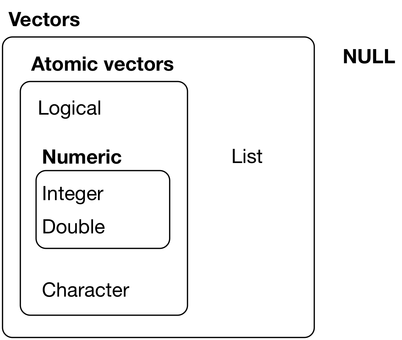{width=400px}](https://r4ds.had.co.nz/vectors.html)
*Credit: [R for Data Science](https://r4ds.had.co.nz/vectors.html)*
Basic **data types**:
- Logical (`TRUE`, `FALSE`)
- Numeric (e.g., `5`, `2.5`)
- Integer (e.g., `1L`, `4L`, where `L` tells R to store as `integer` type)
- Character (e.g., `"R is fun"`)
Basic **data structures**:
- [Atomic vectors](#atomtic-vectors)
- [Lists](#lists)
- [Dataframes](#dataframes)
## Atomtic vectors
What are **atomic vectors**?
- **Atomic vectors** are objects that contains elements
- Elements must be of the same data type (i.e., _homogeneous_)
- The `class()` and `typeof()` a vector describes the elements it contains
**Example**: Investigating logical vectors
```{r}
v <- c(TRUE, FALSE, FALSE, TRUE)
str(v)
class(v)
typeof(v)
```
**Example**: Investigating numeric vectors
```{r}
v <- c(1, 3, 5, 7)
str(v)
class(v)
typeof(v)
```
**Example**: Investigating integer vectors
```{r}
v <- c(1L, 3L, 5L, 7L)
str(v)
class(v)
typeof(v)
```
**Example**: Investigating character vectors
Each element in a `character` vector is a **string** (covered in next section):
```{r}
v <- c("a", "b", "c", "d")
str(v)
class(v)
typeof(v)
```
**Example**: Investigating heterogeneous lists
```{r}
l <- list(2.5, "abc", TRUE, c(1L, 2L, 3L))
str(l)
class(l)
typeof(l)
```
**Example**: Investigating nested lists
```{r}
l <- list(list(TRUE, c(1, 2, 3), list(c("a", "b", "c"))), FALSE, 10L)
str(l)
class(l)
typeof(l)
```
**Example**: Investigating dataframe
```{r}
df <- data.frame(
colA = c(1, 2, 3),
colB = c("a", "b", "c"),
colC = c(TRUE, FALSE, TRUE),
stringsAsFactors = FALSE
)
df
str(df)
class(df)
typeof(df)
```
**Example**: Using `as.logical()` to convert to `logical`
Character vector coerced to logical vector:
```{r}
# Only "TRUE"/"FALSE", "True"/"False", "T"/"F", "true"/"false" are able to be coerced to logical type
as.logical(c("TRUE", "FALSE", "True", "False", "true", "false", "T", "F", "t", "f", ""))
```
Numeric vector coerced to logical vector:
```{r}
# 0 is treated as FALSE, while all other numeric values are treated as TRUE
as.logical(c(0, 0.0, 1, -1, 20, 5.5))
```
**Example**: Using `as.numeric()` to convert to `numeric`
Logical vector coerced to numeric vector:
```{r}
# FALSE is mapped to 0 and TRUE is mapped to 1
as.numeric(c(FALSE, TRUE))
```
Character vector coerced to numeric vector:
```{r, warning = FALSE}
# Strings containing numeric values can be coerced to numeric (leading 0's are dropped)
# All other characters become NA
as.numeric(c("0", "007", "2.5", "abc", "."))
```
**Example**: Using `as.integer()` to convert to `integer`
Logical vector coerced to integer vector:
```{r}
# FALSE is mapped to 0 and TRUE is mapped to 1
as.integer(c(FALSE, TRUE))
```
Character vector coerced to integer vector:
```{r, warning = FALSE}
# Strings containing numeric values can be coerced to integer (leading 0's are dropped, decimals are truncated)
# All other characters become NA
as.integer(c("0", "007", "2.5", "abc", "."))
```
Numeric vector coerced to integer vector:
```{r, warning = FALSE}
# All decimal places are truncated
as.integer(c(0, 2.1, 10.5, 8.8, -1.8))
```
**Example**: Using `as.character()` to convert to `character`
Logical vector coerced to character vector:
```{r}
as.character(c(FALSE, TRUE))
```
Numeric vector coerced to character vector:
```{r, warning = FALSE}
as.character(c(-5, 0, 2.5))
```
Integer vector coerced to character vector:
```{r, warning = FALSE}
as.character(c(-2L, 0L, 10L))
```
**Example**: Using `as.list()` to convert to `list`
Atomic vectors coerced to list:
```{r}
# Logical vector
as.list(c(TRUE, FALSE))
# Character vector
as.list(c("a", "b", "c"))
# Numeric vector
as.list(1:3)
```
**Example**: Using `as.data.frame()` to convert to `data.frame`
Lists coerced to dataframe:
```{r}
# Create a list
l <- list(A = c("x", "y", "z"), B = c(1, 2, 3))
str(l)
# Convert to class `data.frame`
df <- as.data.frame(l, stringsAsFactors = F)
str(df)
```
**Example**: Practical example of converting type
When working with data, it may be helpful to label values for certain variables. Data files often come with a codebook that defines how values are coded. Let's look at an example of labeling values and how converting data type may come into play.
We'll look at the `FIPS` variable from the [Integrated Postsecondary Education Data System (IPEDS)](https://nces.ed.gov/ipeds/use-the-data) data. The [state FIPS code](https://en.wikipedia.org/wiki/Federal_Information_Processing_Standard_state_code#FIPS_state_codes) is a numeric code that identifies a state. For example, `1` is the FIPS code for `Alabama`, `2` is the FIPS code for `Alaska`, etc. We'll want to label each numeric value in the `FIPS` column with the corresponding state name.
```{r}
# Library for labeling variables and values in a dataframe
library(labelled)
# Read in IPEDS data and codebook
ipeds_df <- read.csv('https://raw.githubusercontent.com/cyouh95/recruiting-chapter/master/data/ipeds_hd2017.csv', header = TRUE, na.strings=c('', 'NA'), stringsAsFactors = F)
ipeds_values <- read.csv('https://raw.githubusercontent.com/cyouh95/recruiting-chapter/master/data/ipeds_hd2017_values.csv', header = TRUE, na.strings=c('', 'NA'), stringsAsFactors = F)
# The codebook defines how variables are coded, such as STABBR, FIPS, and other variables
head(ipeds_values)
# Filter codebook for just the values for the FIPS variable
fips_values <- ipeds_values %>% filter(varname == 'FIPS') %>% select(varname, codevalue, valuelabel)
head(fips_values)
```
When we read in the data from the CSV files, R automatically tries to determine the data type of each variable. As seen below, the `FIPS` column from the `ipeds_df` that we want to label is of type `integer`, while the `codevalue` column from the codebook is of type `character` (since not all values are numeric):
```{r}
# Type of `FIPS` column
str(ipeds_df$FIPS)
# Type of `codevalue` column
str(fips_values$codevalue)
```
This discrepancy becomes a problem when we try to label the value using the `labelled` library:
```{r, eval=F}
# Error: `x` and `labels` must be same type
val_label(ipeds_df$FIPS, fips_values[1, 'codevalue']) <- fips_values[1, 'valuelabel']
```
To resolve this, we can use `as.integer()` to convert the `codevalue` from `character` type to `integer` before trying to label the value:
```{r}
# This now works
val_label(ipeds_df$FIPS, as.integer(fips_values[1, 'codevalue'])) <- fips_values[1, 'valuelabel']
# Check value labels
val_labels(ipeds_df$FIPS)
# We can use as.integer() to convert the entire vector (ie. codevalue column) to integer
fips_values$codevalue <- as.integer(fips_values$codevalue)
# Type of `codevalue` column
str(fips_values$codevalue)
# Use loop to label the rest of the values
for (i in 1:nrow(fips_values)) {
val_label(ipeds_df$FIPS, fips_values[i, 'codevalue']) <- fips_values[i, 'valuelabel']
}
# Check value labels
val_labels(ipeds_df$FIPS)
```
**Example**: Creating string using single quotes
Notice how R stores strings using double quotes internally:
```{r}
my_string <- 'This is a string'
my_string
```
**Example**: Creating string using double quotes
```{r}
my_string <- "Strings can also contain numbers: 123"
my_string
```
**Example**: Checking class and type of strings
```{r}
class(my_string)
typeof(my_string)
```
**Note**: To include quotes as part of the string, we can either use the other type of quotes to surround the string (i.e., `'` or `"`) or escape the quote using a backslash (`\`). _We won't be going in-depth into escaping characters for this class, but see appendix for more details if you are interested._
```{r}
# Include quote by using the other type of quotes to surround the string
my_string <- "There's no issues with this string."
my_string
# Include quote of the same type by escaping it with a backslash
my_string <- 'There\'s no issues with this string.'
my_string
```
```{r, eval=F}
# This would not work
my_string <- 'There's an issue with this string.'
my_string
```
# `stringr` package
> "A consistent, simple and easy to use set of wrappers around the fantastic `stringi` package. All function and argument names (and positions) are consistent, all functions deal with `NA`'s and zero length vectors in the same way, and the output from one function is easy to feed into the input of another."
*Credit: `stringr` [R documentation](https://www.rdocumentation.org/packages/stringr/versions/1.4.0)*
The `stringr` package:
- The `stringr` package is based off the `stringi` package and is part of __Tidyverse__
- `stringr` contains functions to work with strings
- For many functions in the `stringr` package, there are equivalent "base R" functions
- But `stringr` functions all follow the same rules, while rules often differ across different "base R" string functions, so we will focus exclusively on `stringr` functions
- Most `stringr` functions start with `str_` (e.g., `str_length`)
## `str_length()`
__The `str_length()` function__:
```{r, eval = FALSE}
?str_length
# SYNTAX
str_length(string)
```
- Function: Find string length
- Arguments:
- `string`: Character vector (or vector coercible to character)
- Note that `str_length()` calculates the length of a string, whereas the `length()` function (which is not part of `stringr` package) calculates the number of elements in an object
**Example**: Using `str_length()` on string
```{r}
str_length("cats")
```
Compare to `length()`, which treats the string as a single object:
```{r}
length("cats")
```
**Example**: Using `str_length()` on character vector
```{r}
str_length(c("cats", "in", "hat"))
```
Compare to `length()`, which finds the number of elements in the vector:
```{r}
length(c("cats", "in", "hat"))
```
**Example**: Using `str_length()` on other vectors coercible to character
Logical vectors can be coerced to character vectors:
```{r}
str_length(c(TRUE, FALSE))
```
Numeric vectors can be coerced to character vectors:
```{r}
str_length(c(1, 2.5, 3000))
```
Integer vectors can be coerced to character vectors:
```{r}
str_length(c(2L, 100L))
```
**Example**: Using `str_length()` on dataframe column
Recall that the columns in a dataframe are just vectors, so we can use `str_length()` as long as the vector is coercible to character type. Let's look at the `screen_name` column from the `p12_df`:
```{r}
# `p12_df` is a dataframe object
str(p12_df)
# `screen_name` column is a character vector
str(p12_df$screen_name)
```
**[Base R method]** Use `str_length()` to calculate the length of each `screen_name`:
```{r}
# Let's focus on just the unique screen names
unique(p12_df$screen_name)
str_length(unique(p12_df$screen_name))
```
**[Tidyverse method]** Use `str_length()` to calculate the length of each `screen_name`:
```{r}
# Let's focus on just the unique screen names
p12_df %>% select(screen_name) %>% unique()
#p12_df %>% select(screen_name) %>% unique() %>% str_length()
```
Notice that the above line does not work as expected because we passed in a dataframe to `str_length()` and it is trying to coerce that to character:
```{r}
class(p12_df %>% select(screen_name) %>% unique())
```
An alternative way is to add a column to the dataframe that contains the result of applying `str_length()` to the `screen_name` vector:
```{r}
p12_df %>% select(screen_name) %>% unique() %>%
mutate(screen_name_len = str_length(screen_name))
```
__The `str_c()` function__:
```{r, eval = FALSE}
?str_c
# SYNTAX AND DEFAULT VALUES
str_c(..., sep = "", collapse = NULL)
```
- Function: Concatenate strings between vectors (element-wise)
- Arguments:
- The input is one or more character vectors (or vectors coercible to character)
- Zero length arguments are removed
- Short arguments are recycled to the length of the longest
- `sep`: String to insert between input vectors
- `collapse`: Optional string used to combine input vectors into single string
**Example**: Using `str_c()` on one vector
Since we only provided one input vector, it has nothing to concatenate with, so `str_c()` will just return the same vector:
```{r}
str_c(c("a", "b", "c"))
```
Note that specifying the `sep` argument will also not have any effect because we only have one input vector, and `sep` is the separator between multiple vectors:
```{r}
str_c(c("a", "b", "c"), sep = "~")
# Check length: Output is the original vector of 3 elements
str_c(c("a", "b", "c")) %>% length()
```
As seen above, `str_c()` returns a vector by default (because the default value for the `collapse` argument is `NULL`). But we can specify a string for `collapse` in order to collapse the elements of the output vector into a single string:
```{r}
str_c(c("a", "b", "c"), collapse = "|")
# Check length: Output vector of length 3 is collapsed into a single string
str_c(c("a", "b", "c"), collapse = "|") %>% length()
# Check str_length: This gives the length of the collapsed string, which is 5 characters long
str_c(c("a", "b", "c"), collapse = "|") %>% str_length()
```
**Example**: Using `str_c()` on more than one vector
When we provide multiple input vectors, we can see that the vectors get concatenated element-wise (i.e., 1st element from each vector are concatenated, 2nd element from each vector are concatenated, etc):
```{r}
str_c(c("a", "b", "c"), c("x", "y", "z"), c("!", "?", ";"))
```
The default separator for each element-wise concatenation is an empty string (`""`), but we can customize that by specifying the `sep` argument:
```{r}
str_c(c("a", "b", "c"), c("x", "y", "z"), c("!", "?", ";"), sep = "~")
# Check length: Output vector is same length as input vectors
str_c(c("a", "b", "c"), c("x", "y", "z"), c("!", "?", ";"), sep = "~") %>% length()
```
Again, we can specify the `collapse` argument in order to collapse the elements of the output vector into a single string:
```{r}
str_c(c("a", "b", "c"), c("x", "y", "z"), c("!", "?", ";"), collapse = "|")
# Check length: Output vector of length 3 is collapsed into a single string
str_c(c("a", "b", "c"), c("x", "y", "z"), c("!", "?", ";"), collapse = "|") %>% length()
# Specifying both `sep` and `collapse`
str_c(c("a", "b", "c"), c("x", "y", "z"), c("!", "?", ";"), sep = "~", collapse = "|")
```
**Example**: Using `str_c()` on "strings"
What do we mean by "strings"?
- Informally, We can think of a "string" as being a character vector with `length()` equal to 1 (i.e., one element).
- Another way to think of it, a "string" is anything you put in between quotes".
- Loosely, we can also think of individual elements within a character vector as strings
Below, passing 3 strings into `str_c()` is like passing in 3 vectors of size 1 each.
- Remember that vectors are concatenated element-wise, so these strings will be joined like this:
```{r}
str_c("a", "b", "c")
# Again, we can think of strings as being character vectors of size 1
str_c(c("a"), c("b"), c("c"))
```
We can use `sep` to specify how the elements are separated:
```{r}
str_c("a", "b", "c", sep = "~")
```
Since we only have 1 element in each vector, the output from `str_c()` is a vector of length 1. Thus, `collapse` will not be useful here since it works to collapse multiple elements in the output vector into a single string:
```{r}
str_c("a", "b", "c", collapse = "|")
```
**Example**: Using `str_c()` on types other than character
When we provide a non-character vector (such as a numeric or logical vector), it will get coerced into a character vector:
```{r}
str_c(c("a", "b", "c"), c(1, 2, 3), c(TRUE, FALSE, FALSE))
# Specifying both `sep` and `collapse`
str_c(c("a", "b", "c"), c(1, 2, 3), c(TRUE, FALSE, FALSE), sep = "~", collapse = "|")
```
Note that we can also use any other single element input (other than string) that can be coerced to character:
```{r}
str_c(TRUE, 1.5, 2L, "X")
```
**Example**: Using `str_c()` on vectors of different lengths
When multiple vectors are provided, they are joined together element-wise, recycling the elements of the shorter vectors:
```{r, warning = FALSE}
str_c("#", c("a", "b", "c", "d"), c(1, 2, 3), c(TRUE, FALSE))
# Specifying both `sep` and `collapse`
str_c("#", c("a", "b", "c", "d"), c(1, 2, 3), c(TRUE, FALSE), sep = "~", collapse = "|")
```
**Example**: Using `str_c()` on dataframe columns
Let's combine the `user_id` and `screen_name` columns from `p12_df`. We'll focus on unique Twitter handles:
```{r}
p12_unique_df <- p12_df %>% select(user_id, screen_name) %>% unique()
p12_unique_df
```
**[Base R method]** Use `str_c()` to combine `user_id` and `screen_name`:
```{r}
str_c(p12_unique_df$user_id, "=", p12_unique_df$screen_name, sep = " ", collapse = ", ")
str_c(p12_unique_df$user_id, "=", p12_unique_df$screen_name, sep = " ") # without collapsing to one element
```
**[Tidyverse method]** Use `str_c()` to combine `user_id` and `screen_name`:
```{r}
p12_unique_df %>% mutate(twitter_handle = str_c(user_id,screen_name))
p12_unique_df %>% mutate(twitter_handle = str_c("User #", user_id, " is @", screen_name))
```
__The `str_sub()` function__:
```{r, eval = FALSE}
?str_sub
# SYNTAX AND DEFAULT VALUES
str_sub(string, start = 1L, end = -1L)
str_sub(string, start = 1L, end = -1L, omit_na = FALSE) <- value
```
- Function: Subset strings
- Arguments:
- `string`: Character vector (or vector coercible to character)
- `start`: Position of first character to be included in substring (default: `1`)
- `end`: Position of last character to be included in substring (default: `-1`)
- Negative index means counting backwards from the end of the string
- If an element in the vector is shorter than the specified `end`, it will just include all the available characters that it does have
- `omit_na`: If `TRUE`, missing values in any of the arguments provided will result in an unchanged input
- When `str_sub()` is used in the assignment form, you can replace the subsetted part of the string with a `value` of your choice
- If an element in the vector is too short to meet the subset specification, the replacement `value` will be concatenated to the end of that element
- Note that this modifies your input vector directly, so you must have the vector saved to a variable (see example below)
**Example**: Using `str_sub()` to subset strings
If no `start` and `end` positions are specified, `str_sub()` will by default return the entire (original) string:
```{r}
str_sub(string = c("abcdefg", 123, TRUE))
```
Note that if an element is shorter than the specified `end` (i.e., `123` in the example below), it will just include all the available characters that it does have:
```{r}
str_sub(string = c("abcdefg", 123, TRUE), start = 2, end = 4)
```
Remember we can also use negative index to count the position starting from the back:
```{r}
str_sub(c("abcdefg", 123, TRUE), start = 2, end = -2)
```
**Example**: Using `str_sub()` to replace strings
If no `start` and `end` positions are specified, `str_sub()` will by default return the original string, so the entire string would be replaced:
```{r}
v <- c("A", "AB", "ABC", "ABCD", "ABCDE")
str_sub(v, start = 1,end =-1)
str_sub(v, start = 1,end =-1) <- "*"
v
```
If an element in the vector is too short to meet the subset specification, the replacement `value` will be concatenated to the end of that element:
```{r}
v <- c("A", "AB", "ABC", "ABCD", "ABCDE")
v
str_sub(v, start = 2, end = 3)
str_sub(v, start = 2, end = 3) <- "*"
v
```
Note that because the replacement form of `str_sub()` modifies the input vector directly, we need to save it in a variable first. Directly passing in the vector to `str_sub()` would give us an error:
```{r, eval = FALSE}
# Does not work
str_sub(c("A", "AB", "ABC", "ABCD", "ABCDE")) <- "*"
```
**Example**: Using `str_sub()` on dataframe column
We can use `as.character()` to turn the `created_at` value to a string, then use `str_sub()` to extract out various date/time components from the string:
```{r}
p12_datetime_df <- p12_df %>% select(created_at) %>%
mutate(
dt_chr = as.character(created_at),
date_chr = str_sub(dt_chr, 1, 10),
yr_chr = str_sub(dt_chr, 1, 4),
mth_chr = str_sub(dt_chr, 6, 7),
day_chr = str_sub(dt_chr, 9, 10),
hr_chr = str_sub(dt_chr, -8, -7),
min_chr = str_sub(dt_chr, -5, -4),
sec_chr = str_sub(dt_chr, -2, -1)
)
p12_datetime_df
```
**Example**: Using `str_to_upper()` to turn strings to uppercase
Turn column names of `p12_df` to uppercase:
```{r}
# Column names are originally lowercase
names(p12_df)
# Turn column names to uppercase
names(p12_df) <- str_to_upper(names(p12_df))
names(p12_df)
```
**Example**: Using `str_to_lower()` to turn strings to lowercase
Turn column names of `p12_df` to lowercase:
```{r}
# Column names are originally uppercase
names(p12_df)
# Turn column names to lowercase
names(p12_df) <- str_to_lower(names(p12_df))
names(p12_df)
```
**Example**: Using `str_sort()` to sort character vector
Sort the vector of `p12_df` column names:
```{r}
# Before sort
names(p12_df)
# Sort alphabetically (default)
str_sort(names(p12_df))
# Sort reverse alphabetically
str_sort(names(p12_df), decreasing = TRUE)
```
**Example**: Using `str_trim()` to trim whitespace from string
```{r}
# Trim whitespace from both left and right sides (default)
str_trim(c("\nABC ", " XYZ\t"))
# Trim whitespace from left side
str_trim(c("\nABC ", " XYZ\t"), side = "left")
# Trim whitespace from right side
str_trim(c("\nABC ", " XYZ\t"), side = "right")
```
**Example**: Using `str_pad()` to pad string with character
Let's say we have a vector of zip codes that has lost all leading 0's. We can use `str_pad()` to add that back in:
```{r}
# Pad the left side of strings with "0" until width of 5 is reached
str_pad(c(95035, 90024, 5009, 5030), width = 5, side = "left", pad = "0")
```
**Example**: Creating `Date` object from character or numeric input
The `lubridate` functions are flexible and can parse dates in various formats:
```{r}
d <- mdy("1/1/2020")
d
d <- mdy("1-1-2020")
d
d <- mdy("Jan. 1, 2020")
d
d <- ymd(20200101)
d
```
Investigate the `Date` object:
```{r}
class(d)
typeof(d)
# Number of days since January 1, 1970
as.numeric(d)
```
**Example**: Creating `POSIXct` object from character or numeric input
The `lubridate` functions are flexible and can parse AM/PM in various formats:
```{r}
dt <- mdy_h("12/31/2019 11pm")
dt
dt <- mdy_hm("12/31/2019 11:59 pm")
dt
dt <- mdy_hms("12/31/2019 11:59:59 PM")
dt
dt <- ymd_hms(20191231235959)
dt
```
Investigate the `POSIXct` object:
```{r}
class(dt)
typeof(dt)
# Number of seconds since January 1, 1970
as.numeric(dt)
```
We can also create a `POSIXct` object from a date function by providing a timezone. The time would default to midnight:
```{r}
dt <- mdy("1/1/2020", tz = "UTC")
dt
# Number of seconds since January 1, 1970
as.numeric(dt) # Note that this is indeed 1 sec after the previous example
```
**Example**: Creating `Date` objects from dataframe column
Using the `p12_datetime_df` we created earlier, we can create `Date` objects from the `date_chr` column:
```{r}
# Use `ymd()` to parse the string stored in the `date_chr` column
p12_datetime_df %>% select(created_at, dt_chr, date_chr) %>%
mutate(date_ymd = ymd(date_chr))
```
**Example**: Creating `POSIXct` objects from dataframe column
Using the `p12_datetime_df` we created earlier, we can recreate the `created_at` column (class `POSIXct`) from the `dt_chr` column (class `character`):
```{r}
# Use `ymd_hms()` to parse the string stored in the `dt_chr` column
p12_datetime_df %>% select(created_at, dt_chr) %>%
mutate(datetime_ymd_hms = ymd_hms(dt_chr))
```
**Example**: Creating `Date` object from individual components
There are various ways to pass in the inputs to create the same `Date` object:
```{r}
d <- make_date(2020, 1, 1)
d
# Characters can be coerced to integers
d <- make_date("2020", "01", "01")
d
# Remember that the default values for month and day would be 1L
d <- make_date(2020)
d
```
**Example**: Creating `POSIXct` object from individual components
```{r}
# Inputs should be numeric
d <- make_datetime(2019, 12, 31, 23, 59, 59)
d
```
**Example**: Creating `Date` objects from dataframe columns
Using the `p12_datetime_df` we created earlier, we can create `Date` objects from the various date component columns:
```{r}
# Use `make_date()` to create a `Date` object from the `yr_chr`, `mth_chr`, `day_chr` fields
p12_datetime_df %>% select(created_at, dt_chr, yr_chr, mth_chr, day_chr) %>%
mutate(date_make_date = make_date(year = yr_chr, month = mth_chr, day = day_chr))
```
**Example**: Creating `POSIXct` objects from dataframe columns
Using the `p12_datetime_df` we created earlier, we can recreate the `created_at` column (class `POSIXct`) from the various date and time component columns (class `character`):
```{r}
# Use `make_datetime()` to create a `POSIXct` object from the `yr_chr`, `mth_chr`, `day_chr`, `hr_chr`, `min_chr`, `sec_chr` fields
# Convert inputs to integers first
p12_datetime_df %>%
mutate(datetime_make_datetime = make_datetime(
as.integer(yr_chr), as.integer(mth_chr), as.integer(day_chr),
as.integer(hr_chr), as.integer(min_chr), as.integer(sec_chr)
)) %>%
select(datetime_make_datetime, yr_chr, mth_chr, day_chr, hr_chr, min_chr, sec_chr)
```
**Example**: Getting date/time components
```{r}
# Create datetime for New Year's Eve
dt <- make_datetime(2019, 12, 31, 23, 59, 59)
dt
dt %>% class()
# Get date
date(dt)
# Get hour
hour(dt)
# Is it pm?
pm(dt)
# Day of the week (3 = Tuesday)
wday(dt)
year(dt)
```
**Example**: Setting date/time components
```{r}
# Create datetime for New Year's Eve
dt <- make_datetime(2019, 12, 31, 23, 59, 59)
dt
# Get week of year
week(dt)
# Set week of year (move back 1 week)
week(dt) <- week(dt) - 1
# Date now moved from New Year's Eve to Christmas Eve
dt
# Set day to Christmas Day
day(dt) <- 25
# Date now moved from Christmas Eve to Christmas Day
dt
```
**Example**: Getting date/time components from dataframe column
Using the `p12_datetime_df` we created earlier, we can isolate the various date/time components from the `POSIXct` object in the `created_at` column:
```{r}
# The extracted date/time components will be of numeric type
p12_datetime_df %>% select(created_at) %>%
mutate(
yr_num = year(created_at),
mth_num = month(created_at),
day_num = day(created_at),
hr_num = hour(created_at),
min_num = minute(created_at),
sec_num = second(created_at),
ampm = ifelse(am(created_at), 'AM', 'PM') # am()/pm() returns TRUE/FALSE
)
```
**Example**: Working with interval
```{r}
# Use `Sys.timezone()` to get timezone for your location (time is midnight by default)
scorpio_start <- ymd("2019-10-23", tz = Sys.timezone())
scorpio_end <- ymd("2019-11-22", tz = Sys.timezone())
scorpio_start
# These datetime objects have class `POSIXct`
class(scorpio_start)
# Create interval for the datetimes
scorpio_interval <- scorpio_start %--% scorpio_end # or `interval(scorpio_start, scorpio_end)`
scorpio_interval <- interval(scorpio_start, scorpio_end)
scorpio_interval
# The object has class `Interval`
class(scorpio_interval)
as.numeric(scorpio_interval)
```
**Example**: Working with period
If we use `as.period()` to get the period of `scorpio_interval`, we see that it is a period of `30` days. We do not worry about the extra `1` hour gained due to daylight savings ending:
```{r}
# Period is 30 days
scorpio_period <- as.period(scorpio_interval)
scorpio_period
# The object has class `Period`
class(scorpio_period)
```
Because periods work with "human" times like days, it is more intuitive. For example, if we add a period of `30` days to the `scorpio_start` datetime object, we get the expected end datetime that is `30` days later:
```{r}
# Start datetime for Scorpio birthdays (time is midnight)
scorpio_start
# After adding 30 day period, we get the expected end datetime (time is midnight)
scorpio_start + days(30)
```
**Example**: Working with duration
If we use `as.duration()` to get the duration of `scorpio_interval`, we see that it is a duration of `2595600` seconds. It takes into account the extra `1` hour gained due to daylight savings ending:
```{r}
# Duration is 2595600 seconds, which is equivalent to 30 24-hr days + 1 additional hour
scorpio_duration <- as.duration(scorpio_interval)
scorpio_duration
# The object has class `Duration`
class(scorpio_duration)
# Using the standard 60s/min, 60min/hr, 24hr/day conversion,
# confirm duration is slightly more than 30 "standard" (ie. 24-hr) days
2595600 / (60 * 60 * 24)
# Specifically, it is 30 days + 1 hour, if we define a day to have 24 hours
seconds_to_period(scorpio_duration)
```
Because durations work with physical time, when we add a duration of `30` days to the `scorpio_start` datetime object, we do not get the end datetime we'd expect:
```{r}
# Start datetime for Scorpio birthdays (time is midnight)
scorpio_start
# After adding 30 day duration, we do not get the expected end datetime
# `ddays(30)` adds the number of seconds in 30 standard 24-hr days, but one of the days has 25 hours
scorpio_start + ddays(30)
# We need to add the additional 1 hour of physical time that elapsed during this time span
scorpio_start + ddays(30) + dhours(1)
```
# Appendix
## Special Characters
> "A sequence in a string that starts with a `\` is called an **escape sequence** and allows us to include special characters in our strings."
*Credit: [Escape sequences](https://campus.datacamp.com/courses/string-manipulation-with-stringr-in-r/string-basics?ex=4) from DataCamp*
**Special characters** are characters that will not be interpreted literally.
Common **special characters**:
- `\n`: newline
- `\t`: tab
- `\`: used for escaping purposes
- `\'`: literal single quote
- `\"`: literal double quote
- `\\`: literal backslash
These characters followed by a backslash `\` take on a new meaning. The `n` by itself is just an `n`. When you add a backslash to the `\n` you are escaping it and making it a special character where `\n` now represents a newline.
__The `writeLines()` function__:
```{r, eval = FALSE}
?writeLines
# SYNTAX AND DEFAULT VALUES
writeLines(text, con = stdout(), sep = "\n", useBytes = FALSE)
```
- "`writeLines()` displays quotes and backslashes as they would be read, rather than as R stores them." (From [writeLines](https://www.rdocumentation.org/packages/base/versions/3.6.2/topics/writeLines) documentation)
- When we include **escape sequences** in the string, it is helpful to use `writeLines()` to see how the escaped string looks
- `writeLines()` will also output the string without showing the outer pair of double quotes that R uses to store it, so we only see the content of the string
**Example**: Escaping single quotes
```{r}
my_string <- 'Escaping single quote \' within single quotes'
my_string
```
Alternatively, we could've just created the string using double quotes:
```{r}
my_string <- "Single quote ' within double quotes does not need escaping"
my_string
```
Using `writeLines()` shows us only the content of the string without the outer pair of double quotes that R uses to store strings:
```{r}
writeLines(my_string)
```
**Example**: Escaping double quotes
```{r}
my_string <- "Escaping double quote \" within double quotes"
my_string
```
Alternatively, we could've just created the string using single quotes:
```{r}
my_string <- 'Double quote " within single quotes does not need escaping'
my_string
```
Notice how the backslash still showed up in the above output to escape our double quote from the outer pair of double quotes that R uses to store the string. This is no longer an issue if we use `writeLines()` to only show the string content:
```{r}
writeLines(my_string)
```
**Example**: Escaping double quotes within double quotes
```{r}
my_string <- "I called my mom and she said \"Echale ganas!\""
my_string
```
Using `writeLines()` shows us only the content of the string without the backslashes:
```{r}
writeLines(my_string)
```
**Example**: Escaping backslashes
To include a literal backslash in the string, we need to escape the backslash with another backslash:
```{r}
my_string <- "The executable is located in C:\\Program Files\\Git\\bin"
my_string
```
Use `writeLines()` to see the escaped string:
```{r}
writeLines(my_string)
```
**Example**: Other special characters
```{r}
my_string <- "A\tB\nC\tD"
my_string
```
Use `writeLines()` to see the escaped string:
```{r}
writeLines(my_string)
```
### Escape special characters using Twitter data
Let's take a look at some tweets from our PAC-12 universities.
- Let's start by grabbing observations 1-3 from the `text` column.
```{r}
#Twitter example of \n newline special characters
p12_df$text[1:3]
```
- Using `writeLines()` we can see the contents of the strings as they would be read, rather than as R stores them.
```{r}
writeLines(p12_df$text[1:3])
```
**Example**: Escaping double quotes using Twitter data
- Using Twitter data you may encounter a lot of strings with double quotes.
- In the example below, our string includes special characters `\"` and `\n` to escape the double quotes and the newline character.
```{r}
#Twitter example of \" double quotes special characters
p12_df$text[24]
```
- Using `writeLines()` we can see the contents of the strings as they would be read, rather than as R stores them.
- We no longer see the escaped characters `\"` or `\n`
```{r}
writeLines(p12_df$text[24])
```