Awesome Spectral Indices in Python:
Numpy |
Pandas |
GeoPandas |
Xarray |
Earth Engine |
Planetary Computer |
Dask |
Cupy |
Cupy-Xarray












---
**GitHub**: [https://github.com/davemlz/spyndex](https://github.com/davemlz/spyndex)
**Documentation**: [https://spyndex.readthedocs.io/](https://spyndex.readthedocs.io/)
**Paper**: [https://doi.org/10.1038/s41597-023-02096-0](https://doi.org/10.1038/s41597-023-02096-0)
**PyPI**: [https://pypi.org/project/spyndex/](https://pypi.org/project/spyndex/)
**Conda-forge**: [https://anaconda.org/conda-forge/spyndex](https://anaconda.org/conda-forge/spyndex)
**Tutorials**: [https://spyndex.readthedocs.io/en/latest/tutorials.html](https://spyndex.readthedocs.io/en/latest/tutorials.html)
---
## Citation
If you use this work, please consider citing the following paper:
```bibtex
@article{montero2023standardized,
title={A standardized catalogue of spectral indices to advance the use of remote sensing in Earth system research},
author={Montero, David and Aybar, C{\'e}sar and Mahecha, Miguel D and Martinuzzi, Francesco and S{\"o}chting, Maximilian and Wieneke, Sebastian},
journal={Scientific Data},
volume={10},
number={1},
pages={197},
year={2023},
publisher={Nature Publishing Group UK London}
}
```
## Overview
The [Awesome Spectral Indices](https://github.com/davemlz/awesome-spectral-indices) is a standardized ready-to-use curated list of spectral indices
that can be used as expressions for computing spectral indices in remote sensing applications. The list was born initially to supply spectral
indices for [Google Earth Engine](https://earthengine.google.com/) through [eemont](https://github.com/davemlz/eemont) and
[spectral](https://github.com/davemlz/spectral), but given the necessity to compute spectral indices for other object classes outside the Earth
Engine ecosystem, a new package was required.
Spyndex is a python package that uses the spectral indices from the *Awesome Spectral Indices* list and creates an expression evaluation method that is
compatible with python object classes that support [overloaded operators](https://docs.python.org/3/reference/datamodel.html#emulating-numeric-types)
(e.g. [numpy.ndarray](https://github.com/numpy/numpy), [pandas.Series](https://github.com/pandas-dev/pandas),
[xarray.DataArray](https://github.com/pydata/xarray)).
Some of the `spyndex` features are listed here:
- Access to Spectral Indices from the Awesome Spectral Indices list.
- Multiple Spectral Indices computation.
- Kernel Indices computation.
- Parallel processing.
- Compatibility with a lot of python objects!
Check the simple usage of spyndex here:
```python
import spyndex
import numpy as np
import xarray as xr
N = np.random.normal(0.6,0.10,10000)
R = np.random.normal(0.1,0.05,10000)
da = xr.DataArray(
np.array([N,R]).reshape(2,100,100),
dims = ("band","x","y"),
coords = {"band": ["NIR","Red"]}
)
idx = spyndex.computeIndex(
index = ["NDVI","SAVI"],
params = {
"N": da.sel(band = "NIR"),
"R": da.sel(band = "Red"),
"L": 0.5
}
)
```
Bands can also be passed as keywords arguments:
```python
idx = spyndex.computeIndex(
index = ["NDVI","SAVI"],
N = da.sel(band = "NIR"),
R = da.sel(band = "Red"),
L = 0.5
)
```
And indices can be computed from their class:
```python
idx = spyndex.indices.NDVI.compute(
N = da.sel(band = "NIR"),
R = da.sel(band = "Red"),
)
```
## How does it work?
Any python object class that supports overloaded operators can be used with spyndex methods.
---
*"Hey... what do you mean by 'overloaded operators'?"*
---
That's the million dollars' question! An object class that supports overloaded operators is the one that allows you to compute mathematical
operations using common operators (`+`, `-`, `/`, `*`, `**`) like `a + b`, `a + b * c` or `(a - b) / (a + b)`. You know the last one, right? That's
the formula of the famous [NDVI](https://doi.org/10.1016/0034-4257(79)90013-0).
So, if you can use the overloaded operators with an object class, you can use that class with [spyndex](https://github.com/davemlz/spyndex)!
> BE CAREFUL! Not all overloaded operators work as mathematical operators. In a `list` object class, the addition operator (`+`) concatenates two objects instead of performing an addition operation! So you must convert the `list` into a `numpy.ndarray` before using spyndex!
Here is a little list of object classes that support mathematical overloaded operators:
- `float` (Python Built-in type) or `numpy.float*` (with [numpy](https://github.com/numpy/numpy))
- `int` (Python Built-in type) or `numpy.int*` (with [numpy](https://github.com/numpy/numpy))
- `numpy.ndarray` (with [numpy](https://github.com/numpy/numpy))
- `pandas.Series` (with [pandas](https://github.com/pandas-dev/pandas) or [geopandas](https://github.com/geopandas/geopandas))
- `xarray.DataArray` (with [xarray](https://github.com/pydata/xarray))
- `ee.Image` (with [earthengine-api](https://github.com/google/earthengine-api) and [eemont](https://github.com/davemlz/eemont))
- `ee.Number` (with [earthengine-api](https://github.com/google/earthengine-api) and [eemont](https://github.com/davemlz/eemont))
And wait, there is more! If objects that support overloaded operatores can be used in spyndex, that means that you can work in **parallel**
with [dask](https://docs.dask.org/en/latest/)!
Here is the list of the dask objects that you can use with spyndex:
- `dask.Array` (with the `dask-array` extra)
- `dask.Series` (with the `dask-dataframe` extra)
BUT WAIT! THERE IS EVEN MORE! If you want **GPU-accelerated computing**, you can use [cupy](https://cupy.dev/)!
- `cupy.ndarray` (with [cupy](https://cupy.dev/) or with [cupy-xarray](https://github.com/xarray-contrib/cupy-xarray))
This means that you can actually use spyndex in a lot of processes! For example, you can download a Sentinel-2 image with
[sentinelsat](https://github.com/sentinelsat/sentinelsat), open and read it with [rasterio](https://github.com/mapbox/rasterio) and then compute
the desired spectral indices with [spyndex](https://github.com/davemlz/spyndex). Or you can search through the Landsat-8 STAC in the
[Planetary Computer](https://planetarycomputer.microsoft.com/) ecosystem using [pystac-client](https://github.com/stac-utils/pystac-client),
convert it to an `xarray.DataArray` with [stackstac](https://github.com/gjoseph92/stackstac) and then compute spectral indices using
[spyndex](https://github.com/davemlz/spyndex) in parallel with [dask](https://docs.dask.org/en/latest/) or with GPU acceleration using [cupy](https://cupy.dev/)! Amazing, right!?
## Installation
Install the latest version from PyPI:
```
pip install spyndex
```
Install support for an optional array or dataframe library:
```
pip install "spyndex[numpy]"
pip install "spyndex[pandas]"
pip install "spyndex[xarray]"
pip install "spyndex[dask-array]"
pip install "spyndex[dask-dataframe]"
```
Plotting support is available with `pip install "spyndex[plot]"`, and Earth
Engine support with `pip install "spyndex[ee]"`.
Upgrade spyndex by running:
```
pip install -U spyndex
```
Install the latest version from conda-forge:
```
conda install -c conda-forge spyndex
```
Install the latest dev version from GitHub by running:
```
pip install git+https://github.com/davemlz/spyndex
```
## Features
### Exploring Spectral Indices
Spectral Indices from the Awesome Spectral Indices list can be accessed through
`spyndex.indices`. This is a `Box` object where each one of the indices in the list
can be accessed as well as their [attributes](https://github.com/davemlz/awesome-ee-spectral-indices#attributes):
```python
import spyndex
# All indices
spyndex.indices
# NDVI index
spyndex.indices["NDVI"]
# Or with dot notation
spyndex.indices.NDVI
# Formula of the NDVI
spyndex.indices["NDVI"]["formula"]
# Or with dot notation
spyndex.indices.NDVI.formula
# Reference of the NDVI
spyndex.indices["NDVI"]["reference"]
# Or with dot notation
spyndex.indices.NDVI.reference
```
### Default Values
Some Spectral Indices require constant values in order to be computed. Default values
can be accessed through `spyndex.constants`. This is a `Box` object where each one
of the [constants](https://github.com/davemlz/awesome-spectral-indices#expressions) can be
accessed:
```python
import spyndex
# All constants
spyndex.constants
# Canopy Background Adjustment
spyndex.constants["L"]
# Or with dot notation
spyndex.constants.L
# Default value
spyndex.constants["L"]["default"]
# Or with dot notation
spyndex.constants.L.default
```
### Band Parameters
The standard band parameters description can be accessed through `spyndex.bands`. This is
a `Box` object where each one of the [bands](https://github.com/davemlz/awesome-spectral-indices#expressions)
can be accessed:
```python
import spyndex
# All bands
spyndex.bands
# Blue band
spyndex.bands["B"]
# Or with dot notation
spyndex.bands.B
```
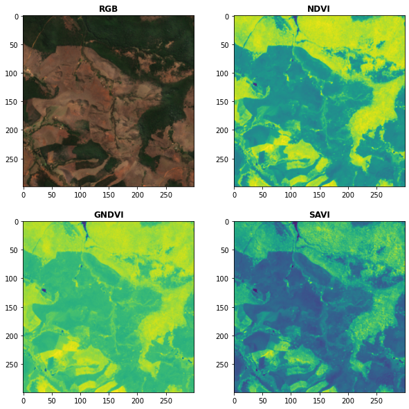
### One (or more) Spectral Indices Computation
Use the `computeIndex()` method to compute as many spectral indices as you want!
The `index` parameter receives the spectral index or a list of spectral indices to
compute, while the `params` parameter receives a dictionary with the
[required parameters](https://github.com/davemlz/awesome-ee-spectral-indices#expressions)
for the spectral indices computation.
```python
import spyndex
import xarray as xr
import matplotlib.pyplot as plt
from rasterio import plot
# Open a dataset (in this case a xarray.DataArray)
snt = spyndex.datasets.open("sentinel")
# Scale the data (remember that the valid domain for reflectance is [0,1])
snt = snt / 10000
# Compute the desired spectral indices
idx = spyndex.computeIndex(
index = ["NDVI","GNDVI","SAVI"],
params = {
"N": snt.sel(band = "B08"),
"R": snt.sel(band = "B04"),
"G": snt.sel(band = "B03"),
"L": 0.5
}
)
# Plot the indices (and the RGB image for comparison)
fig, ax = plt.subplots(2,2,figsize = (10,10))
plot.show(snt.sel(band = ["B04","B03","B02"]).data / 0.3,ax = ax[0,0],title = "RGB")
plot.show(idx.sel(index = "NDVI").data,ax = ax[0,1],title = "NDVI")
plot.show(idx.sel(index = "GNDVI").data,ax = ax[1,0],title = "GNDVI")
plot.show(idx.sel(index = "SAVI").data,ax = ax[1,1],title = "SAVI")
```
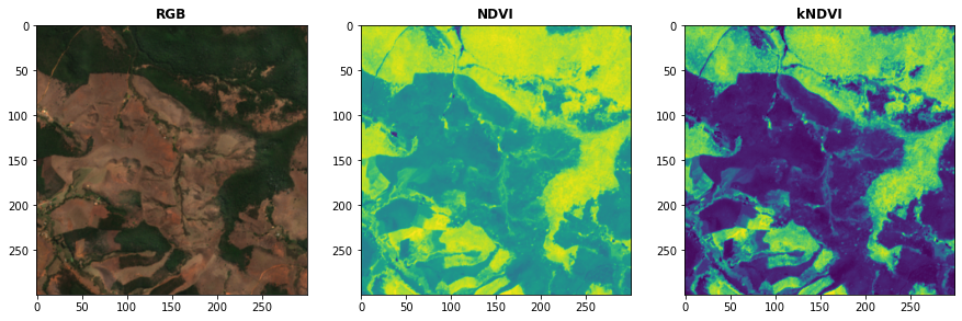
### Kernel Indices Computation
Use the `computeKernel()` method to compute the required kernel for kernel indices like
the kNDVI! The `kernel` parameter receives the kernel to compute, while the `params`
parameter receives a dictionary with the
[required parameters](https://github.com/davemlz/awesome-ee-spectral-indices#expressions)
for the kernel computation (e.g., `a`, `b` and `sigma` for the RBF kernel).
```python
import spyndex
import xarray as xr
import matplotlib.pyplot as plt
from rasterio import plot
# Open a dataset (in this case a xarray.DataArray)
snt = spyndex.datasets.open("sentinel")
# Scale the data (remember that the valid domain for reflectance is [0,1])
snt = snt / 10000
# Compute the kNDVI and the NDVI for comparison
idx = spyndex.computeIndex(
index = ["NDVI","kNDVI"],
params = {
# Parameters required for NDVI
"N": snt.sel(band = "B08"),
"R": snt.sel(band = "B04"),
# Parameters required for kNDVI
"kNN" : 1.0,
"kNR" : spyndex.computeKernel(
kernel = "RBF",
params = {
"a": snt.sel(band = "B08"),
"b": snt.sel(band = "B04"),
"sigma": snt.sel(band = ["B08","B04"]).mean("band")
}),
}
)
# Plot the indices (and the RGB image for comparison)
fig, ax = plt.subplots(1,3,figsize = (15,15))
plot.show(snt.sel(band = ["B04","B03","B02"]).data / 0.3,ax = ax[0],title = "RGB")
plot.show(idx.sel(index = "NDVI").data,ax = ax[1],title = "NDVI")
plot.show(idx.sel(index = "kNDVI").data,ax = ax[2],title = "kNDVI")
```
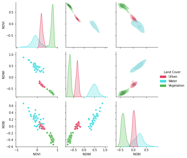
### A `pandas.DataFrame`? Sure!
No matter what kind of python object you're working with, it can be used with `spyndex` as long as it supports mathematical overloaded operators!
```python
import spyndex
import pandas as pd
import seaborn as sns
import matplotlib.pyplot as plt
# Open a dataset (in this case a pandas.DataFrame)
df = spyndex.datasets.open("spectral")
# Compute the desired spectral indices
idx = spyndex.computeIndex(
index = ["NDVI","NDWI","NDBI"],
params = {
"N": df["SR_B5"],
"R": df["SR_B4"],
"G": df["SR_B3"],
"S1": df["SR_B6"]
}
)
# Add the land cover column to the result
idx["Land Cover"] = df["class"]
# Create a color palette for plotting
colors = ["#E33F62","#3FDDE3","#4CBA4B"]
# Plot a pairplot to check the indices behaviour
plt.figure(figsize = (15,15))
g = sns.PairGrid(idx,hue = "Land Cover",palette = sns.color_palette(colors))
g.map_lower(sns.scatterplot)
g.map_upper(sns.kdeplot,fill = True,alpha = .5)
g.map_diag(sns.kdeplot,fill = True)
g.add_legend()
plt.show()
```
### Parallel Processing
Parallel processing is possible with `spyndex` and `dask`! You can use `dask.array` or `dask.dataframe` objects to compute spectral indices with spyndex!
If you're using `xarray`, you can also define a chunk size and work in parallel!
```python
import spyndex
import numpy as np
import dask.array as da
# Define the array shape
array_shape = (10000,10000)
# Define the chunk size
chunk_size = (1000,1000)
# Create a dask.array object
dask_array = da.array([
da.random.normal(0.6,0.10,array_shape,chunks = chunk_size),
da.random.normal(0.1,0.05,array_shape,chunks = chunk_size)
])
# "Compute" the desired spectral indices
idx = spyndex.computeIndex(
index = ["NDVI","SAVI"],
params = {
"N": dask_array[0],
"R": dask_array[1],
"L": 0.5
}
)
# Since dask works in lazy mode,
# you have to tell it that you want to compute the indices!
idx.compute()
```
### Using `cupy`
You want GPU-accelerated computing? Well, that's also possible with `spyndex` and `cupy` (and with `cupy-xarray` too!).
Try it with `cupy`:
```python
import spyndex
import cupy as cp
# cupy.ndarray objects
N = cp.random.normal(0.6,0.10,10000)
R = cp.random.normal(0.1,0.05,10000)
# Returns a cupy.ndarray object
idx = spyndex.computeIndex(
index = "NDVI",
N = N,
R = R
)
```
Try it with `cupy-xarray`:
```python
import spyndex
import xarray as xr
import cupy_xarray
# Open a dataset (in this case a xarray.DataArray)
snt = spyndex.datasets.open("sentinel")
# Convert it to a dataset of cupy.ndarray objects
snt_cupy = snt.cupy.as_cupy()
# Scale the data (remember that the valid domain for reflectance is [0,1])
snt_cupy = snt_cupy / 10000
# Compute the desired spectral indices
idx_cupy = spyndex.computeIndex(
index = ["NDVI","GNDVI","SAVI"],
params = {
"N": snt_cupy.sel(band = "B08"),
"R": snt_cupy.sel(band = "B04"),
"G": snt_cupy.sel(band = "B03"),
"L": 0.5
}
)
# Convert back to numpy!
idx = idx_cupy.as_numpy()
```
### Plotting Spectral Indices
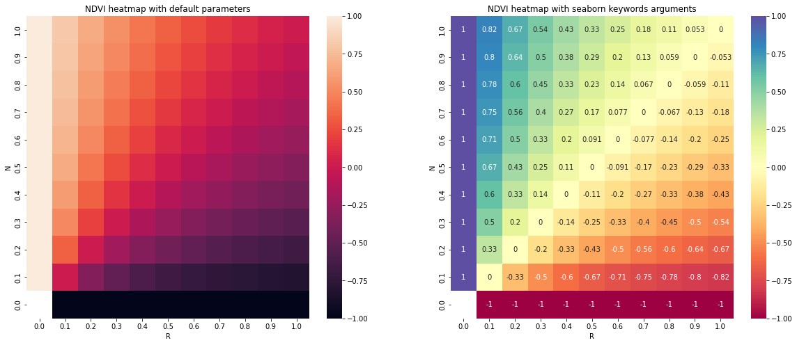
All posible values of a spectral index can be visualized using `spyndex.plot.heatmap()`! This is a module that doesn't require data,
just specify the index, the bands, and BOOM! Heatmap of all the possible values of the index!
```python
import spyndex
import matplotlib.pyplot as plt
import seaborn as sns
# Define subplots grid
fig, ax = plt.subplots(1,2,figsize = (20,8))
# Plot the NDVI with the Red values on the x-axis and the NIR on the y-axis
ax[0].set_title("NDVI heatmap with default parameters")
spyndex.plot.heatmap("NDVI","R","N",ax = ax[0])
# Keywords arguments can be passed for sns.heatmap()
ax[1].set_title("NDVI heatmap with seaborn keywords arguments")
spyndex.plot.heatmap("NDVI","R","N",annot = True,cmap = "Spectral",ax = ax[1])
plt.show()
```
## License
The project is licensed under the MIT license.
## Contributing
Check the [contributing page](https://spyndex.readthedocs.io/en/latest/contributing.html).