GEOG 172: INTERMEDIATE GEOGRAPHICAL ANALYSIS

Evgeny Noi

Lecture 07: Inferential Statistics and Hypothesis Testing

Statistical Testing

• We are broadly interested in mean of a neighborhood and comparing it to the overall mean of the city
• It is expensive to sample / survey entire city, so we would like to develop methdolology that could tell us how likely we are to find the values

Setting up our hypotheses

• Null hypothesis: the mean of the neighborhood $\mu=3.1$.
• Alternative
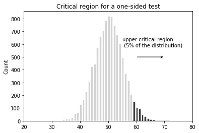
  • $\mu > 3.1$ (one sided test)
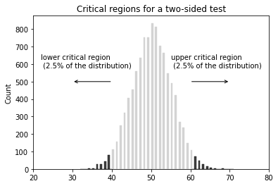
  • $\mu \neq 3.1$

Sample Probability

• We sample 10 households in the neighborhood and find that $\mu=11.1$
• How can we relate this value to our 'true' mean?
  • Null is TRUE, but we have obtained an unusual sample
  • Null is FALSE

The role of statistic is to quantify how unusual it would be to obtain our sample if the null hypothesis was true

Judge Analogy

• Think about a judge judging a defendant.
• Judge begins by presuming innocence. The judge must decide whether there is sufficient evidence to reject the presumed innocence of the defendant (beyond a reasonable doubt).
• A judge can err, however, by convicting a defendant who is innocent, or by failing to convict one who is actually guilty.
• In similar fashion, the investigator starts by presuming the null hypothesis, or no association between the predictor and outcome variables in the population.
• Based on the data collected in his sample, the investigator uses statistical tests to determine whether there is sufficient evidence to reject the null hypothesis in favor of the alternative hypothesis that there is an association in the population. The standard for these tests is shown as the level of statistical significance.

Source: Banerjee A, Chitnis UB, Jadhav SL, Bhawalkar JS, Chaudhury S. Hypothesis testing, type I and type II errors. Ind Psychiatry J. 2009 Jul;18(2):127-31. doi: 10.4103/0972-6748.62274. PMID: 21180491; PMCID: PMC2996198.

Error Types in Hypothesis Testing

• Type I - rejecting a true hypothesis (denoted by $\alpha$, typically set at 0.01, 0.05, and 0.1). False positive
• Type II - accepting a false hypothesis False negative

Errors

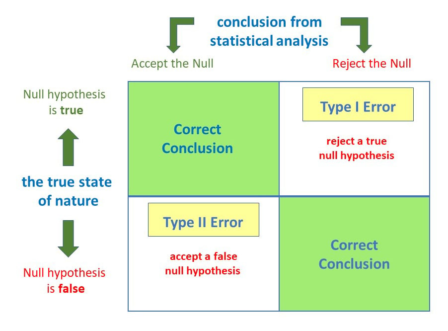
Errors (examples)

• Null is true, the mean in the urban area is indeed 3.1 (as demonstrated on the sample).
  • Reject true null (Type I error): $\alpha$ (False positive, i.e. 'falsely rejecting true null')
  • Accept true null: $1 - \alpha$ (True Positive)
• Null is false, the mean in the urban area is not 3.1 (biased sample, wrong conjecture in the first place, rare event).
  • Reject false null: $1 - \beta$ (True negative)
  • Accept false null (Type II error): $\beta$ (False negative, i.e. 'falsely accepting false null')

We can decrease the magnitude of errors by increasing a sample size!

Inferential Terminology

• Random variable (RV) - variable that takes on different values determined by chance.
• RVs can be discrete (countable) and continuous (line).
• Probability function - mathematical function that provides probabilities for possible outcomes of the RV ($f(x)$)
• The probability function for discrete RV is called Probability Mass Function (PMF). $f(x) = P(X=x)$ and $f(x)>0$ and $\sum f(x)=1$ (sum of probs sum to 1).
• The probability function for continuous RV is called Probability Density Function (PDF). $f(x) \neq P(X=x)$. and $f(x)>0$ with area under curve equal to 1.
• Cumulative Density Function ($F(x)$) - probability that RV, $X \leq x$.

Expected Value and Variance

• Expected value (mean) and variance. $\mu = E(X) = \sum x_i f(x_i)$. Multiply each value $x$ in the support by its respective probability ($f(x)$) and add them up. Average value weighted by the likelihood.
• Variance: $\sigma^2 = Var(X) = \sum(x_i - \mu)^2 f(x_i) = \sum x_i^2 f(x_i) - \mu^2$
• Standard deviation: $\sigma = SD(X) = \sqrt{VAR}(X) = \sqrt{\sigma^2}$

In statistics, we use $\sigma$ to denote population SD and $s$ to denote sample SD.

Distributions

• Each distribution can be defined based on its PMF/PDF.

Binomial Distribution

RV with two outcomes. We have $n$ trials and $p/\pi$ - success probability.

• $f(x) = \frac{n!}{x!(n-x)!}p^x(1-p)^{n-x} \quad for \quad x = 0,1,2,...,n$
• Mean: $\mu=np$,
• Variance: $\sigma^2=np(1-p)$

# A company drills 9 wild-cat oil exploration wells, each with an estimated probability 
# of success of 0.1. All nine wells fail. What is the probability of that happening?
import numpy as np

n, p, sample = 9, .1, 20000 
pct = np.sum(np.random.binomial(n, p, sample) == 0)/20000

print(f'The probability that all 9 wells fail: {round(pct,3)*100}%')

The probability that all 9 wells fail: 39.0%

PMF for Binomial Distribution

Normal Distribution

• $N(\mu, \sigma^2)$. A standard normal distibution is parameterized by $N(0,1$ and is also known as the $z$ distribution.
• $f(x) = \frac{1}{\sigma \sqrt{2\pi}}e^{-\frac{1}{2}(\frac{x-\mu}{\sigma})^2}$
• Any normal RV can be transformed into a standard normal RV by finding the z-score. Then use stasndard normal tables.
• Z-score can be positive, negative. We can use $z$ to identify outliers (+/-3), max possible $z=\frac{n-1}{\sqrt{n}}$

$$ Z = \frac{\text{Observed value - mean}}{SD} $$

Plotted PDF for Normal Distribution

Exercise 1

According to Center for Disease Control, heights for US adult males and females are approximately normal

• Females ($\mu=64$ inches and $SD=2$ inches)
• Males ($\mu=69$ inches and $SD=3$ inches)

1. Convert your height to $z$-score
2. What is the probability of a randomly selected US adult female being shorted than 65 inches?

Answer

Find $P(X<65)$

$$ z = \frac{65-64}{2} = 0.5 $$

Equivalently, find $P(Z<0.50)$ from the table (0.6915). So, roughly there this a 69% chance that a randomly selected U.S. adult female would be shorter than 65 inches.

Sampling Distribution

The sampling distribution of a statistic is a probability distribution based on a large number of samples of size from a given population.

---

Consider a situation. We need to measure the average length of fish in the hatchery. We a certain number of fish into the tank and sample randomly from the tank, measuring and recording mean at each attempt ($\bar{x_1}, \bar{x_2}, \bar{x_3}, ... \bar{x_n}$).

from numpy.random import default_rng
rng = default_rng(12345) # ensure replicability with seed
list_of_means, list_of_data = [], []

for i in np.arange(0,100):
    vals = rng.uniform(low=0.5, high=6.0, size=1000)
    list_of_means.append(np.mean(vals))
    list_of_data.append(vals)
    
plt.hist(list_of_means);
plt.axvline(np.mean(list_of_means), color='red', lw=3, linestyle='dashed', label='mean of means')
plt.title('Sampling Distribution of Means \n drawn from Uniform Distribution', fontsize=16);
plt.legend();

import seaborn as sns
import pandas as pd

dff = pd.DataFrame(list_of_data)
dff = dff.T#.to_numpy().flatten()

fig, ax=plt.subplots(1,2, figsize=(12,4))

dff.plot(kind='hist', color='b', alpha=.1, ax=ax[0], legend=False);
sns.histplot(list_of_means,ax=ax[1]);

Test Statistic

• Test statistic will be normally distributed for samples drawn from normal or near normal distribution

$$ z = \frac{\bar{x}-\mu}{\frac{\sigma}{\sqrt{n}}} $$

where $SD = \frac{\sigma}{\sqrt{n}}$

Exercise 2

The engines made by Ford for speedboats have an average power of 220 horsepower (HP) and standard deviation of 15 HP. You can assume the distribution of power follows a normal distribution.

Consumer Reports® is testing the engines and will dispute the company's claim if the sample mean is less than 215 HP. If they take a sample of 4 engines, what is the probability the mean is less than 215?

How to solve

1. Draw a normal distribution
2. Find the mean. Which direction do we need to explore?
3. Find the $z$ value, look up area under curve for $z$

Answer

$$ SD = \frac{15}{\sqrt{4}}=7.5 $$$$ P(\bar{X} < 215) = P \Big( Z < \frac{215-220}{7.5} \Big) = P(Z<-0.67) \approx 0.2514 $$

Central Limit Theorem (CLT)

For a large sample size $\bar{x}$ is approximately normally distributed, regardless of the distribution of the population one samples from. If the population has mean $\mu$ and standard deviation $\sigma$, then $\bar{x}$ has mean $\mu$ and standard deviation $\frac{\sigma}{\sqrt{n}}$

he Central Limit Theorem applies to a sample mean from any distribution. We could have a left-skewed or a right-skewed distribution. As long as the sample size is large, the distribution of the sample means will follow an approximate Normal distribution. Samples size of at least 30 is considered large.

Clear explanation at StatQuest

Types of Statistical Inferences

• Estimation - using information from the sample to estimate / predict parameters of interest (estimate median income in urban area)
  • point estimates (one value)
  • interval estimates (confidence intervals) - An interval of values computed from sample data that is likely to cover the true parameter of interest. Including a measure of confidence with our estimate forms a margin of error (the median income in the area is 33,450 $\pm$ 1,532.
• Statistical (Hypothesis) tests - using information from the sample to determine whether a certain statement about the parameter of interest is true (find out if the median income in urban area is above \$30,000).

General form of a confidence intervals and MOE

$$ \text{sample statistic} \pm \text{margin of error} $$$$ \text{Margin of Error} = M \times \hat{SE}\text{(estimate)} $$

where $M$ is a multiplier, based on how confidence we are in our estimate.

The interpretation of a confidence interval has the basic template of: "We are 'some level of percent confident' that the 'population of interest' is from 'lower bound to upper bound'.

Inference for the population mean

• We would like to derive a point estimate of the population mean $\mu$. For this, we need to calculate point estimate of the sample mean $\bar{x}$.

Constructing and interpreting CI

• When $\sigma$ is known
  • the $(1-\alpha)$100\% confidence interval for $\mu$ is: $\bar{x} \pm z_{\alpha/2} \frac{\sigma}{\sqrt{n}}$
• When $\sigma$ is unknown:
  • Estimate statistic via $t$-distribution $t = \frac{\bar{X}-\mu}{\frac{s}{\sqrt{n}}}$. t-Table
  • the $(1-\alpha)$100\% confidence interval for $\mu$ is: $\bar{x} \pm t_{\alpha/2} \frac{\sigma}{\sqrt{n}}$

Exercise 3

You are interested in the average emergency room (ER) wait time at your local hospital. You take a random sample of 50 patients who visit the ER over the past week. From this sample, the mean wait time was 30 minutes and the standard deviation was 20 minutes. Find a 95% confidence interval for the average ER wait time for the hospital.

1. Is the data normal and is the sample large enough?
2. Locate $t$-value in the table and plug into your formula for CI

Answer

Use $\alpha=0.05/2$ for columns in the table and df=40 for rows. The $t$-value is 2.021.

$$ \begin{align} CI &= \bar{x} \pm t{\alpha/2}\frac{s}{\sqrt{n}} \\ &= 30 \pm 2.021 \frac{20}{\sqrt{50}} \\ &= (24.28, 35.72) \end{align} $$

We are 95% confident that mean emergency room wait time at our local hospital is from 24.28 minutes to 35.72 minutes.

Checking Normality in Python

• Use tips dataset from Seaborn

One waiter recorded information about each tip he received over a period of a few months working in one restaurant. He collected several variables:

tips = sns.load_dataset("tips")
tips

	total_bill	tip	sex	smoker	day	time	size
0	16.99	1.01	Female	No	Sun	Dinner	2
1	10.34	1.66	Male	No	Sun	Dinner	3
2	21.01	3.50	Male	No	Sun	Dinner	3
3	23.68	3.31	Male	No	Sun	Dinner	2
4	24.59	3.61	Female	No	Sun	Dinner	4
...	...	...	...	...	...	...	...
239	29.03	5.92	Male	No	Sat	Dinner	3
240	27.18	2.00	Female	Yes	Sat	Dinner	2
241	22.67	2.00	Male	Yes	Sat	Dinner	2
242	17.82	1.75	Male	No	Sat	Dinner	2
243	18.78	3.00	Female	No	Thur	Dinner	2

244 rows × 7 columns

fig, ax = plt.subplots(1,2, figsize=(12,4))
sns.histplot(data=tips, x='total_bill', ax=ax[0]);
sns.histplot(data=tips, x='tip', ax=ax[1]);

import statsmodels.api as sm
import scipy

fig, ax = plt.subplots(1,2, figsize=(12,4))

sm.qqplot(tips.total_bill, line='45', ax=ax[0], fit=True);
sm.qqplot(rng.normal(size=1000), line='45', ax=ax[1]);

# calculating cofnidence intervals 
import statsmodels.stats.api as sms

ci = sms.DescrStatsW(tips.total_bill).tconfint_mean()

print(f"The confidence interval for tips is {ci}")

The confidence interval for tips is (18.663331704358473, 20.908553541543167)

Penguins Data

Source

pengs = sns.load_dataset("penguins")
pengs

	species	island	bill_length_mm	bill_depth_mm	flipper_length_mm	body_mass_g	sex
0	Adelie	Torgersen	39.1	18.7	181.0	3750.0	Male
1	Adelie	Torgersen	39.5	17.4	186.0	3800.0	Female
2	Adelie	Torgersen	40.3	18.0	195.0	3250.0	Female
3	Adelie	Torgersen	NaN	NaN	NaN	NaN	NaN
4	Adelie	Torgersen	36.7	19.3	193.0	3450.0	Female
...	...	...	...	...	...	...	...
339	Gentoo	Biscoe	NaN	NaN	NaN	NaN	NaN
340	Gentoo	Biscoe	46.8	14.3	215.0	4850.0	Female
341	Gentoo	Biscoe	50.4	15.7	222.0	5750.0	Male
342	Gentoo	Biscoe	45.2	14.8	212.0	5200.0	Female
343	Gentoo	Biscoe	49.9	16.1	213.0	5400.0	Male

344 rows × 7 columns

sns.pairplot(pengs, corner=True, diag_kind='kde')

<seaborn.axisgrid.PairGrid at 0x2b4118cab90>

from scipy import stats
def quantile_plot(x, **kwargs):
    quantiles, xr = stats.probplot(x, fit=False)
    plt.scatter(xr, quantiles, **kwargs)

g = sns.FacetGrid(pengs, height=4)
g.map(quantile_plot, "body_mass_g")

<seaborn.axisgrid.FacetGrid at 0x2b40f3a7610>

pengs.body_mass_g.mean()

4201.754385964912

Hypothesis Testing (Continued)

1. Check normality and sample size for tips (good on both)
2. Set up hypotheses
3. Decide on significance level $\alpha$
4. Calculate test statistic and/or $p$-value
5. Make decision about null hypothesis

P-value

$p$-value is defined to be the smallest Type I error rate ($\alpha$) that you have to be willing to tolerate if you want to reject the null hypothesis.

$p$-value (or probability value) is the probability that the test statistic equals the observed value or a more extreme value under the assumption that the null hypothesis is true.

If our p-value is less than or equal to $\alpha$, then there is enough evidence to reject the null hypothesis. If our p-value is greater than $\alpha$, there is not enough evidence to reject the null hypothesis.

Demo

• Check Normality
• Set-up hypotheses: $H_0$: $\mu = 4201$ AND $H_a$: $\mu \neq 4201$ (two-tailed test)
• $\alpha=0.05$

from scipy import stats

print(stats.ttest_1samp(pengs.body_mass_g.dropna(), popmean=4201))
print('Our p-value is not below alpha, thus we cannot reject the null hypothesis.')
print(f'We are 95% confident, that the population mean body weight of penguins is indeed 4201 grams')

Ttest_1sampResult(statistic=0.01739630065824133, pvalue=0.9861306342800811)
Our p-value is not below alpha, thus we cannot reject the null hypothesis.
We are 95% confident, that the population mean body weight of penguins is indeed 4201 grams

Demo 2

• $H_0$: $\mu \leq 1000$ AND $H_a$: $\mu > 1000$ (one-tailed test)
• $\alpha=0.05$

from scipy import stats

print(stats.ttest_1samp(pengs.body_mass_g.dropna(), popmean=1000, alternative='greater'))
print('Our p-value is below **alpha**, thus we cannot accept the null hypothesis.')
print('We are 95% confident, that the population mean body weight of penguins is greater than 1000 grams')

Ttest_1sampResult(statistic=73.83313651463514, pvalue=4.1249540274922355e-212)
Our p-value is below **alpha**, thus we cannot accept the null hypothesis.
We are 95% confident, that the population mean body weight of penguins is greater than 1000 grams

Independent Samples $t$-test

Use for comparing the mean of two groups

Does flipper length vary depending on the sex of the penguin?

sns.histplot(data=pengs, x="flipper_length_mm", hue="sex", element='step')

<AxesSubplot:xlabel='flipper_length_mm', ylabel='Count'>

import pingouin as pg

ax = pg.qqplot(pengs.flipper_length_mm, dist='norm')

from scipy.stats import shapiro

shapiro(pengs.flipper_length_mm.dropna()) # p-val<0.05 - departure from normality

ShapiroResult(statistic=0.9517050385475159, pvalue=5.392858604125195e-09)

sns.pointplot(x = 'sex', y = 'flipper_length_mm', data = pengs)
sns.despine()

from pingouin import ttest
pengs.dropna(inplace=True)

ttest(pengs.loc[pengs.sex=='Male', 'flipper_length_mm'], pengs.loc[pengs.sex=='Female', 'flipper_length_mm']) 

	T	dof	alternative	p-val	CI95%	cohen-d	BF10	power
T-test	4.807866	325.278352	two-sided	0.000002	[4.22, 10.06]	0.526244	5880.711	0.997654

# amend for normality via Wilcoxon
pg.mwu(pengs.loc[pengs.sex=='Male', 'flipper_length_mm'], pengs.loc[pengs.sex=='Female', 'flipper_length_mm'], alternative='two-sided')

	U-val	alternative	p-val	RBC	CLES
MWU	18173.0	two-sided	9.011341e-07	-0.311183	0.655592

Potential Problems

• Non-normality of data (bi-modal)
• Homogeneity of variance

References:

Banerjee, A., Chitnis, U. B., Jadhav, S. L., Bhawalkar, J. S., & Chaudhury, S. (2009). Hypothesis testing, type I and type II errors. Industrial psychiatry journal, 18(2), 127.

Rogerson, P. A. (2019). Statistical methods for geography: a student’s guide. Sage.

Penn State STAT 500: Applied Statistics Course Materials

Learning Statistics with Python