GEOG 172: INTERMEDIATE GEOGRAPHICAL ANALYSIS

Evgeny Noi

Lecture 8: Comparing Means (t-tests and ANOVA)

Last Lecture Review (Distributions)

• RV can be continuous (PDF) and discrete (PMF)
• Each distribution can be parametrized by their corresponding density functions

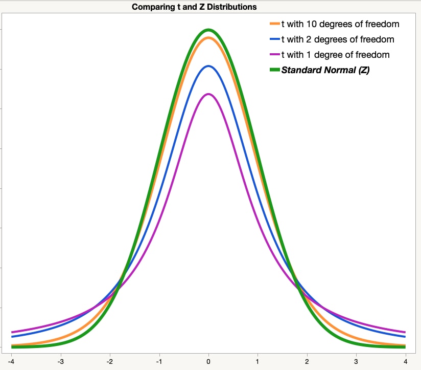
Last Lecture Review ($z$ and $t$)

• We can convert normally distributed RVs into standard normal distribution ($z$-score)
• We can use the $z$-score to assess probability of observing data at or below the $z$. Use the $z$-table to look up probability values.
• We use $t$ when the population SD is not known (most real-life situations) or when sample size is below 30. Use the $t$-table to look up probability values.

$z$-score

$$ z = \frac{\bar{x}-\mu}{\frac{\sigma}{\sqrt{n}}} $$

$t$-score

$$ t = \frac{\bar{x}-\mu}{\frac{s}{\sqrt{n}}} $$

where $s$ is the sample variance, $\sigma$ is the population variance, $\bar{x}$ is the sample mean, and $\mu$ is the population mean.

Last Lecture Review (CI)

• We can estimate population mean ($\mu$) and variance ($\sigma^2$) from sample mean ($\bar{x}$) and sample variance ($s^2$)
• We can provide confidence intervals for population mean using formulas $\bar{x} \pm t_{\alpha/2} \frac{s}{\sqrt{n}}$ with $df=n-1$
• Interpret the CI: We are $(1-\alpha)100%$ sure that the population mean, $\mu$, is between $\bar{x} - t_{\alpha/2} \frac{s}{\sqrt{n}}$ and $\bar{x} + t_{\alpha/2} \frac{s}{\sqrt{n}}$

Last Lecture Review (QQ-Plot)

In statistics, a Q–Q plot (quantile-quantile plot) is a probability plot, a graphical method for comparing two probability distributions by plotting their quantiles against each other. If the two distributions being compared are similar, the points in the Q–Q plot will approximately lie on the identity line $y = x$.

Last Lecture Review (Hypotheses)

• Null hypothesis - is assumed to be true until there is evidence to suggest otherwise.
• Alternative hypothesis - research hypotehsis.

The goal of hypothesis testing is to see if there is enough evidence against the null hypothesis. If there is not enough evidence, then we fail to reject the null hypothesis

Last Lecture Review (Errors)

• Null is true, the mean in the urban area is indeed 3.1 (as demonstrated on the sample).
  • Reject true null (Type I error): $\alpha$ (False positive, i.e. 'falsely rejecting true null')
  • Accept true null: $1 - \alpha$ (True Positive)
• Null is false, the mean in the urban area is not 3.1 (biased sample, wrong conjecture in the first place, rare event).
  • Reject false null: $1 - \beta$ (True negative)
  • Accept false null (Type II error): $\beta$ (False negative, i.e. 'falsely accepting false null')

We can decrease the magnitude of errors by increasing a sample size!

Six Steps of Hypothesis Tests

1. Set up hypothesis and check conditions (normality, independence)
2. Decide on the significance level $\alpha$ (probability cutoff for making decisions about null hypothesis). The probability we are willing to place on our test for making an incorrect decision rejecting the null hypothesis.
3. Calculate test statistic.

Six Steps of Hypothesis Tests

1. Calculate probability value ($p$-value) or find the rejection region
2. Make decision about the null (reject of fail to reject)
3. State overall conclusion.

Setting-up Hypothesis Tests

• Is the population mean different from $\mu_0$? (Two-tailed, non-directional)
  • $H_0$: $\mu = \mu_0$
  • $H_a$: $\mu \neq \mu_0$
• Is the population mean greater than $\mu_0$? (Right-tailed, directional)
  • $H_0$: $\mu = \mu_0$
  • $H_a$: $\mu > \mu_0$
• Is the population mean less than $\mu_0$? (Left-tailed, directional)
  • $H_0$: $\mu = \mu_0$
  • $H_a$: $\mu < \mu_0$

One Sample t-Tests

Steps 1-3

• Set up hypothesis (see previous slide) and set $\mu_0=8.5$ (hypothesized population mean). The data comes from normal distribution of size = 30
• $\alpha=0.05$
• Calculate the test statistic

Steps 4-6 (Critical Region)

• Find critical values (tables). Rejection regions:
  • left-handed: reject $H_0$ if $t^* \leq t_{\alpha}$
  • right-handed: reject $H_0$ if $t^* \geq t_{\alpha}$
  • two-tailed: reject $H_0$ if $|t^*| \geq |t_{\alpha/2}|$
• Make decision about the null
• State an overall conclusion

Steps 4-6 ($p$-values)

• Computing p-value
  • If $H_a$ is right-tailed, then the p-value is the probability the sample data produces a value equal to or greater than the observed test statistic. $P(t\leq t^*)$
  • If $H_a$ is left-tailed, then the p-value is the probability the sample data produces a value equal to or less than the observed test statistic. $P(t\geq t^*)$
  • If $H_a$ is two-tailed, then the p-value is two times the probability the sample data produces a value equal to or greater than the absolute value of the observed test statistic. $2 \times P(t\geq |t^*|)$
• Make decision about the null. If the p-value is less than the significance level, $\alpha$, then reject $H_0$ (and conclude $H_a$)
• State an overall conclusion

Example

The mean length of the lumber is supposed to be 8.5 feet. A builder wants to check whether the shipment of lumber she receives has a mean length different from 8.5 feet. If the builder observes that the sample mean of 61 pieces of lumber is 8.3 feet with a sample standard deviation of 1.2 feet. What will she conclude? Is 8.3 very different from 8.5?

$$ \begin{align} t^* &= \frac{\bar{x}-\mu}{\frac{s}{\sqrt{n}}} \\ &= \frac{8.3-8.5}{\frac{1.2}{\sqrt{61}}} \\ &= -1.3 \end{align} $$

Thus, we are asking if $-1.3$ is very far away from zero, since that corresponds to the case when $\bar{x}$ is equal to $\mu_0$. If it is far away, then it is unlikely that the null hypothesis is true and one rejects it. Otherwise, one cannot reject the null hypothesis.

1. $H_0$: $\mu = 8.5$; $H_a$: $\mu \neq 8.5$
2. $\alpha=.01$
3. $t^* = -1.3$

Rejection region approach

1. $df = 61-60 = 60$, the critical value is $t_{\alpha/2} = 2.660$, thus $t^*$ is not within $\pm 2.660$
2. $t^*$ is not within rejection region, we fail to reject null hypothesis.
3. With a test statistic of $-1.3$ and critical value of $\pm 2.660$ at a 1\% level of significance, we do not have enough statistical evidence to reject the null hypothesis. We conclude that there is not enough statistical evidence that indicates that the mean length of lumber differs from $8.5$ feet.

P-value approach

1. Without software to find a more exact probability, the best we can do from the t-table is find a range. We do see that the value falls between 1.296 and 1.671. These two t-values correspond to right-tail probabilities of 0.1 and 0.05, respectively. Since 1.3 is between these two t-values, then it stands to reason that the probability to the right of 1.3 would fall between 0.05 and 0.1. Therefore, the p-value would be = 2×(0.05 and 0.1) or from 0.1 to 0.2.
2. Fail to reject the null
3. With a test statistic of - 1.3 and p-value between 0.1 to 0.2, we fail to reject the null hypothesis at a 1% level of significance since the p-value would exceed our significance level. We conclude that there is not enough statistical evidence that indicates that the mean length of lumber differs from 8.5 feet.

P-value

$p$-value is defined to be the smallest Type I error rate ($\alpha$) that you have to be willing to tolerate if you want to reject the null hypothesis.

$p$-value (or probability value) is the probability that the test statistic equals the observed value or a more extreme value under the assumption that the null hypothesis is true.

If our p-value is less than or equal to $\alpha$, then there is enough evidence to reject the null hypothesis. If our p-value is greater than $\alpha$, there is not enough evidence to reject the null hypothesis.

Penguins Data

Source

import seaborn as sns
penguins = sns.load_dataset("penguins")
penguins

	species	island	bill_length_mm	bill_depth_mm	flipper_length_mm	body_mass_g	sex
0	Adelie	Torgersen	39.1	18.7	181.0	3750.0	MALE
1	Adelie	Torgersen	39.5	17.4	186.0	3800.0	FEMALE
2	Adelie	Torgersen	40.3	18.0	195.0	3250.0	FEMALE
3	Adelie	Torgersen	NaN	NaN	NaN	NaN	NaN
4	Adelie	Torgersen	36.7	19.3	193.0	3450.0	FEMALE
...	...	...	...	...	...	...	...
339	Gentoo	Biscoe	NaN	NaN	NaN	NaN	NaN
340	Gentoo	Biscoe	46.8	14.3	215.0	4850.0	FEMALE
341	Gentoo	Biscoe	50.4	15.7	222.0	5750.0	MALE
342	Gentoo	Biscoe	45.2	14.8	212.0	5200.0	FEMALE
343	Gentoo	Biscoe	49.9	16.1	213.0	5400.0	MALE

344 rows × 7 columns

import matplotlib.pyplot as plt
g = sns.pairplot(penguins, corner=True, diag_kind='kde')
g.fig.set_size_inches(4,4)

penguins.body_mass_g.dropna().plot(kind='hist')

<AxesSubplot: ylabel='Frequency'>

One sample test for penguins

• $H_0$: the mean body mass of penguins is 4201 grams
• $H_a$: the mean body mass of penguins is not 4201

What kind of t-test is this?

from scipy import stats

print(stats.ttest_1samp(penguins.body_mass_g.dropna(), popmean=4201))
print('Our p-value is not below alpha, thus we cannot reject the null hypothesis.')
print(f'We do not have enough statistical evidence to reject the null hypothesis.')
print('We conclude that there is not enough statistical evidence that indicates that the mean\n mass of penguins differs from  4201 g.')

Ttest_1sampResult(statistic=0.01739630065824133, pvalue=0.9861306342800811)
Our p-value is not below alpha, thus we cannot reject the null hypothesis.
We do not have enough statistical evidence to reject the null hypothesis.
We conclude that there is not enough statistical evidence that indicates that the mean
 mass of penguins differs from  4201 g.

One sample test for penguins (v2)

• $H_0$: the mean body mass of penguins is 4300 grams
• $H_a$: the mean body mass of penguins is less than 4300

What kind of t-test is this?

from scipy import stats

print(stats.ttest_1samp(penguins.body_mass_g.dropna(), popmean=4300, alternative='less'))
print('Our p-value is below **alpha**, thus we cannot accept the null hypothesis.')
print(f'We do not have enough statistical evidence to accept the null hypothesis.')
print('We conclude that there is enough statistical evidence that indicates that the mean\n mass of penguins is less than 4300 g.')

Ttest_1sampResult(statistic=-2.265564736887436, pvalue=0.012052359189978712)
Our p-value is below **alpha**, thus we cannot accept the null hypothesis.
We do not have enough statistical evidence to accept the null hypothesis.
We conclude that there is enough statistical evidence that indicates that the mean
 mass of penguins is less than 4300 g.

Independent Samples t-Test

• Let's assume that our penguins data is a combination of two independent samples: one for male penguins and another for female penguins.
• We can use a $t$-test to compare the means between the groups and state whether those are statistically different from one another.
• Be a good data scientist and check normality assumptions on the data sample.

BIG QUESTION: Does flipper length vary depending on the sex of the penguin?

# QQPLOT 
import pingouin as pg
ax = pg.qqplot(penguins.flipper_length_mm, dist='norm')

# Shapiro-Wilk test
from scipy.stats import shapiro
shapiro(penguins.flipper_length_mm.dropna()) # p-val<0.05 - departure from normality

ShapiroResult(statistic=0.9515460133552551, pvalue=3.541138271501154e-09)

Our data is not normal, but we will still proceed with the outlined tests to demonstrate Python functionality.

We will see later what tests to use when we see non-normal data

# visualize difference with a plot
sns.pointplot(x = 'sex', y = 'flipper_length_mm', data = penguins)
sns.despine()

Comparing means between independendent samples

SAMPLES ARE NOT PAIRED AND NOT RELATED IN ANY WAY TO ANOTHER!

Pooled standard deviation:

$$ s_p = \sqrt{\frac{(n_1-1)s_1^2 + (n_2-1)s_2^2}{n1+n2-2}} $$

Sample stastistic (Unpooled Variance)

$$ t = \frac{\bar{x_1} - \bar{x_2} - 0}{s_p \sqrt{\frac{1}{n_1} + \frac{1}{n_2}}} $$

Confidence intervals

$$ \bar{x}_1-\bar{x}_2\pm t_{\alpha/2}s_p\sqrt{\frac{1}{n_1}+\frac{1}{n_2}} $$

Hypothesis tests

• $H_0$: $\mu_1 - \mu_2 = 0$; $H_a$: $\mu_1 - \mu_2 \neq 0$, with $df=n_1+n_2 - 2$

penguins

	species	island	bill_length_mm	bill_depth_mm	flipper_length_mm	body_mass_g	sex
0	Adelie	Torgersen	39.1	18.7	181.0	3750.0	MALE
1	Adelie	Torgersen	39.5	17.4	186.0	3800.0	FEMALE
2	Adelie	Torgersen	40.3	18.0	195.0	3250.0	FEMALE
4	Adelie	Torgersen	36.7	19.3	193.0	3450.0	FEMALE
5	Adelie	Torgersen	39.3	20.6	190.0	3650.0	MALE
...	...	...	...	...	...	...	...
338	Gentoo	Biscoe	47.2	13.7	214.0	4925.0	FEMALE
340	Gentoo	Biscoe	46.8	14.3	215.0	4850.0	FEMALE
341	Gentoo	Biscoe	50.4	15.7	222.0	5750.0	MALE
342	Gentoo	Biscoe	45.2	14.8	212.0	5200.0	FEMALE
343	Gentoo	Biscoe	49.9	16.1	213.0	5400.0	MALE

333 rows × 7 columns

from pingouin import ttest, mwu
penguins.dropna(inplace=True) # drop null values 
males = penguins.loc[penguins.sex=='MALE', 'flipper_length_mm']
females = penguins.loc[penguins.sex=='FEMALE', 'flipper_length_mm'] 
print(males.shape, females.shape)
ttest(males, females) 

(168,) (165,)

	T	dof	alternative	p-val	CI95%	cohen-d	BF10	power
T-test	4.807866	325.278352	two-sided	0.000002	[4.22, 10.06]	0.526244	5880.711	0.997654

# use Mann-Whitney non-parametric test (to account for non-normal data)
mwu(males, females, alternative='two-sided')

	U-val	alternative	p-val	RBC	CLES
MWU	18173.0	two-sided	9.011341e-07	-0.311183	0.655592

Interpreting

With a $p$-value of 9.011e-07 we have enough evidence to reject null hypothesis. The average flipper length between male and female penguins is different.

Comparing two population variances

• $H_0$: $\frac{\sigma_1^2}{\sigma_2^2}=1$; $H_a$: $\frac{\sigma_1^2}{\sigma_2^2} \neq 1$
• F-test: assumes two samples come from populations that are normally distributed
• Bartlett's test
• Levene's test

from scipy.stats import bartlett
stat, p = bartlett(males, females)
print(f'the p-value: {p}')
print('populations have equal variances at alpha=0.05')

the p-value: 0.05197230787956047
populations have equal variances at alpha=0.05

ANOVA

Analysis of Variance

Hypothesis Testing

• We are ONCE AGAIN comparing MEANS from $t$ different samples
• $H_0$: $\mu_1 = \mu_2 = ... = \mu_k$
• at least one mean is different OR not all the means are equal

Test statistic for a One-Way ANOVA

$$ F = \frac{\text{between group variance}}{\text{within group variance}} = \frac{MS_{\text{effect}}}{MS_{\text{error}}} $$

Under the null, the $F$ should be close to 1, if the ratio is large, we have evidence against teh null.

Variance

$$ \mbox{Var}(Y) = \frac{1}{N} \sum_{k=1}^G \sum_{i=1}^{N_k} \left(Y_{ik} - \bar{Y} \right)^2 $$

where $G$ is the number of groups, $N$ is the number of observations (penguins), Y_{ik} is the total body mass of k-group (species) of an $i$th individual

Sum of Squares

$$ \mbox{SS}_{tot} = \sum_{k=1}^G \sum_{i=1}^{N_k} \left(Y_{ik} - \bar{Y} \right)^2 \quad \text{- total sum of squares} $$$$ \mbox{SS}_w = \sum_{k=1}^G \sum_{i=1}^{N_k} \left( Y_{ik} - \bar{Y}_k \right)^2 \quad \text{- within-group SS} $$$$ {SS}_{b} = \sum_{k=1}^{G} \sum_{k=1}^G N_k \left( \bar{Y}_k - \bar{Y} \right)^2 $$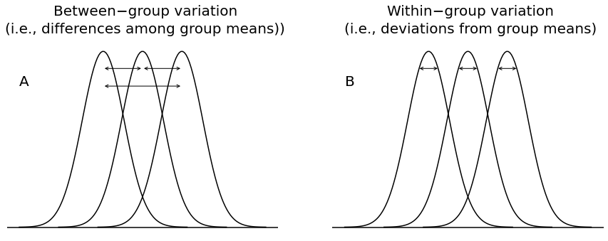

$$ \mbox{SS}_w + \mbox{SS}_{b} = \mbox{SS}_{tot} $$

From SS to an F-test

• $df_b = G-1$, $df_w = N-G$
• $MS_b = \frac{SS_b}{df_b}$, $MS_w = \frac{SS_w}{df_w}$
• $F=\frac{MS_b}{MS_w}$

ANOVA assumptions

• Responses for each factor level have normal population distribution
• the distributions have the same variance
• the data are independent!

penguins.groupby('species')['body_mass_g'].agg(['mean', 'std', 'size'])

	mean	std	size
species
Adelie	3706.164384	458.620135	146
Chinstrap	3733.088235	384.335081	68
Gentoo	5092.436975	501.476154	119

sns.boxplot(data=penguins, x='species', y='body_mass_g', hue='sex')

<AxesSubplot: xlabel='species', ylabel='body_mass_g'>

#ANOVA 
import pingouin as pg
penguins.anova(dv='body_mass_g', between='species', detailed=False)

C:\Users\barguzin\Anaconda3\envs\geo_env\lib\site-packages\pingouin\parametric.py:992: FutureWarning: Not prepending group keys to the result index of transform-like apply. In the future, the group keys will be included in the index, regardless of whether the applied function returns a like-indexed object.
To preserve the previous behavior, use

	>>> .groupby(..., group_keys=False)

To adopt the future behavior and silence this warning, use 

	>>> .groupby(..., group_keys=True)
  sserror = grp.apply(lambda x: (x - x.mean()) ** 2).sum()

	Source	ddof1	ddof2	F	p-unc	np2
0	species	2	330	341.894895	3.744505e-81	0.674489

# ANOVA VIA SCIPY 
import scipy.stats as stats
# stats f_oneway functions takes the groups as input and returns ANOVA F and p value
fvalue, pvalue = stats.f_oneway(penguins.loc[penguins.species=='Adelie', 'body_mass_g'], 
                                penguins.loc[penguins.species=='Chinstrap', 'body_mass_g'], 
                                penguins.loc[penguins.species=='Gentoo', 'body_mass_g'])
print(fvalue, pvalue)

341.8948949481461 3.74450512630046e-81

import statsmodels.api as sm
from statsmodels.formula.api import ols

model = ols('body_mass_g ~ C(species)', data=penguins).fit()
anova_table = sm.stats.anova_lm(model, typ=2)
anova_table

	sum_sq	df	F	PR(>F)
C(species)	1.451902e+08	2.0	341.894895	3.744505e-81
Residual	7.006945e+07	330.0	NaN	NaN

Questions?

References

Banerjee, A., Chitnis, U. B., Jadhav, S. L., Bhawalkar, J. S., & Chaudhury, S. (2009). Hypothesis testing, type I and type II errors. Industrial psychiatry journal, 18(2), 127.

Rogerson, P. A. (2019). Statistical methods for geography: a student’s guide. Sage.

Penn State STAT 500: Applied Statistics Course Materials

Learning Statistics with Python