GEOG 172: INTERMEDIATE GEOGRAPHICAL ANALYSIS

Evgeny Noi

Lecture 12: More on Clustering and Clusters

Review

• LISA separates the data into two groups:
  • local clusters
  • local outliers
• Motivating question: How can we assess spatial patterns in point data?
  • Point pattern analysis (centrography, quadrant analysis)
  • Clustering

Airbnb Data

Amsterdam

We will download the file from the website you've been working with to access the data for Lab 6. To be able to run the code below, you need to install a Python distribution of wget (e.g. pip install wget). Command 'wget' runs natively on Unix-based systems (e.g. Linux and MacOS), but if you are on Windows, we need to work around it.

!python -m wget http://data.insideairbnb.com/the-netherlands/north-holland/amsterdam/2022-09-07/visualisations/listings.csv

Saved under listings (1).csv

!python -m wget http://data.insideairbnb.com/the-netherlands/north-holland/amsterdam/2022-09-07/visualisations/neighbourhoods.geojson

Saved under neighbourhoods (1).geojson

import pandas as pd
import geopandas as gpd
import numpy as np 
import matplotlib.pyplot as plt
import contextily as cx
from pointpats import (
    distance_statistics,
    QStatistic,
    random,
    PointPattern,
)

geo = gpd.read_file('neighbourhoods.geojson') 
print(geo.shape) 
print(geo.crs) 
df = pd.read_csv('listings.csv') 
print(df.shape) 

(22, 3)
epsg:4979
(6893, 18)

df.head()

	id	name	host_id	host_name	neighbourhood_group	neighbourhood	latitude	longitude	room_type	price	minimum_nights	number_of_reviews	last_review	reviews_per_month	calculated_host_listings_count	availability_365	number_of_reviews_ltm	license
0	2818	Quiet Garden View Room & Super Fast WiFi	3159	Daniel	NaN	Oostelijk Havengebied - Indische Buurt	52.36435	4.94358	Private room	49	3	305	2022-08-30	1.86	1	14	25	0363 5F3A 5684 6750 D14D
1	20168	Studio with private bathroom in the centre 1	59484	Alexander	NaN	Centrum-Oost	52.36407	4.89393	Private room	106	1	339	2020-04-09	2.22	2	0	0	0363 CBB3 2C10 0C2A 1E29
2	27886	Romantic, stylish B&B houseboat in canal district	97647	Flip	NaN	Centrum-West	52.38761	4.89188	Private room	136	2	231	2022-04-24	1.78	1	121	8	0363 974D 4986 7411 88D8
3	28871	Comfortable double room	124245	Edwin	NaN	Centrum-West	52.36775	4.89092	Private room	75	2	428	2022-08-24	2.92	2	117	75	0363 607B EA74 0BD8 2F6F
4	29051	Comfortable single room	124245	Edwin	NaN	Centrum-Oost	52.36584	4.89111	Private room	55	2	582	2022-08-29	4.16	2	160	86	0363 607B EA74 0BD8 2F6F

# convert pd to gpd 
bnb_pts = gpd.GeoDataFrame(
    df, crs='epsg:4326', geometry=gpd.points_from_xy(df['longitude'], df['latitude']))

coordinates = df[['longitude', 'latitude']].values
random_pattern = random.poisson(coordinates, size=1000)

f, ax = plt.subplots()
plt.scatter(*random_pattern.T, color="r", marker="x", label="Random", alpha=.5)
bnb_pts.sample(1000).plot(markersize=5,ax=ax, alpha=.5, label='observed');
cx.add_basemap(ax, crs=bnb_pts.crs.to_string())
ax.legend();

qstat = QStatistic(coordinates)
print('P-value:', qstat.chi2_pvalue)
qstat.plot()

P-value: 0.0

qstat_null = QStatistic(random_pattern)
print('P-value:', qstat_null.chi2_pvalue)
qstat_null.plot()

P-value: 0.8502021603566939

Words of Caution with Quadrant Analysis

• Quadrat counts are measured in a regular tiling that is overlaid on top of the potentially irregular extent of our pattern. Thus, irregular but random patterns can be mistakenly found 'significant'

import libpysal

alpha_shape, alpha, circs = libpysal.cg.alpha_shape_auto(coordinates, return_circles=True)
random_pattern_ashape = random.poisson(alpha_shape, size=1000)

qstat_null_ashape = QStatistic(random_pattern_ashape)
print('P-value:', qstat_null_ashape.chi2_pvalue)
qstat_null_ashape.plot()

P-value: 2.4002518827238188e-57

Ripley's Functions

• Characterize clustering and co-location of point patterns
• Look at nearest neighbor distances between each point and their neighbors at different distance tresholds
• The plot denotes cumulative percentage against the increasing distance radii
• Observed cumulative distribution is compared against a reference (spatially random) distribution (Poisson point process)

Ripley's $G$ Function (event-to-event)

$$ G(d) = \sum_{i=1}^n \frac{ \phi_i^d}{n} $$

$G(d)$ is the proportion of nearest neighbor distances that are less than $d$.

$$ \phi_i^d = \begin{cases} 1 & \quad \text{if } d_{min}(s_i)<d \\ 0 & \quad \text{otherwise } \\ \end{cases} $$

# the dataset is large (we need to resample) for computational purposes 
n=500
index = np.random.choice(coordinates.shape[0], n, replace=False)  
print(index.shape)

g_test = distance_statistics.g_test(
    coordinates[index], support=40, keep_simulations=True
)

(500,)

Ripley's $G$ intuition

• Distance between points
• In distributions of distances, a clustered pattern must have more points near one another than a pattern that is dispersed; and a completely random pattern should have something in between.
• If the function increases rapidly with distance, we probably have a clustered pattern. If it increases slowly with distance, we have a dispersed pattern. Something in the middle will be difficult to distinguish from pure chance.

f, ax = plt.subplots(
    1, 2, figsize=(9, 3), gridspec_kw=dict(width_ratios=(6, 3))
)
# plot all the simulations with very fine lines
ax[0].plot(
    g_test.support, g_test.simulations.T, color="k", alpha=0.01
)
# and show the average of simulations
ax[0].plot(
    g_test.support,
    np.median(g_test.simulations, axis=0),
    color="cyan",
    label="median simulation",
)


# and the observed pattern's G function
ax[0].plot(
    g_test.support, g_test.statistic, label="observed", color="red"
)

# clean up labels and axes
ax[0].set_xlabel("distance")
ax[0].set_ylabel("% of nearest neighbor\ndistances shorter")
ax[0].legend()
#ax[0].set_xlim(0, 2000)
ax[0].set_title(r"Ripley's $G(d)$ function")

# plot the pattern itself on the next frame
ax[1].scatter(*coordinates[index].T)

# and clean up labels and axes there, too
ax[1].set_xticks([])
ax[1].set_yticks([])
ax[1].set_xticklabels([])
ax[1].set_yticklabels([])
ax[1].set_title("Pattern")
f.tight_layout()
f.savefig('Ripley_G.png')
plt.close()

from IPython.display import Image
Image(filename='Ripley_G.png') 

Ripley's $F$ function (point-event)

• analyzing the distance to points in the pattern from locations in empty space (the 'empty space function')
• $F$ accumulates, for a growing distance range, the percentage of points that can be found within that range from a random point pattern generated within the extent of the observed pattern
• If the pattern has large gaps or empty areas, the function will increase slowly. But, if the pattern is highly dispersed, then the function will increase rapidly.

f_test = distance_statistics.f_test(
    coordinates[index], support=40, keep_simulations=True
)

f, ax = plt.subplots(
    1, 2, figsize=(9, 3), gridspec_kw=dict(width_ratios=(6, 3))
)
# plot all the simulations with very fine lines
ax[0].plot(
    f_test.support, f_test.simulations.T, color="k", alpha=0.01
)
# and show the average of simulations
ax[0].plot(
    f_test.support,
    np.median(f_test.simulations, axis=0),
    color="cyan",
    label="median simulation",
)


# and the observed pattern's G function
ax[0].plot(
    f_test.support, f_test.statistic, label="observed", color="red"
)

# clean up labels and axes
ax[0].set_xlabel("distance")
ax[0].set_ylabel("% of nearest neighbor\ndistances shorter")
ax[0].legend()
#ax[0].set_xlim(0, 2000)
ax[0].set_title(r"Ripley's $F(d)$ function")

# plot the pattern itself on the next frame
ax[1].scatter(*coordinates[index].T)

# and clean up labels and axes there, too
ax[1].set_xticks([])
ax[1].set_yticks([])
ax[1].set_xticklabels([])
ax[1].set_yticklabels([])
ax[1].set_title("Pattern")
f.tight_layout()
f.savefig('Ripley_F.png')
plt.close()

from IPython.display import Image
Image(filename='Ripley_F.png') 

# alternatively 
from pointpats import PointPattern
print(pointpats.__version__)

pp = PointPattern(coordinates[index]) # creates a point pattern plot 
ffun = distance_statistics.F(pp, intervals=15)
gfun = distance_statistics.G(pp, intervals=15)

2.2.0

gfun.plot()

Ripley's $K$ function

• Considers distance to higher order neighbors (between all pairs of of event points)

$$ K(d) = \frac{\sum_{i=1}^n \sum_{j=1}^n \psi_{ij}(d)}{n \hat{\lambda}} $$

where

$$ \psi_{ij}(d) = \begin{cases} 1 & \quad \text{if } d_{ij}<d \\ 0 & \quad \text{otherwise } \\ \end{cases} $$

$\sum \psi_{id}(d)$ is the number of events within a circle of radius d centered on event si

kfun = distance_statistics.K(pp, intervals=15)

kfun.plot()

Identifying Clusters via Density

• DBSCAN (Density-Based Spatial Clustering of Applications) - algorithm from knowledge discovery and machine learning.
• DBSCAN is deterministic (there is no associated inferential framework as in LISA). Thus, we cannot relate it to CSR.

DBSCAN

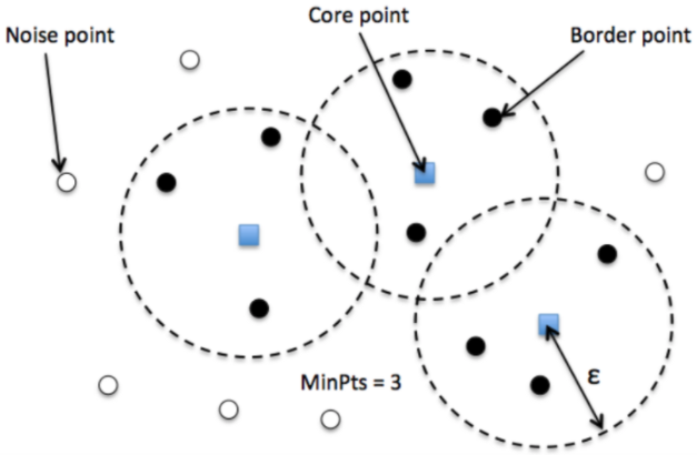
• Cluster is a concentration of at least $m$ points, each of them within a distance $r$ of at least another point in cluster (both $m$ and $r$ must be specified by a user).
• DBSCAN patterns:
  • Noise, for those points outside a cluster.
  • Cores, for those points inside a cluster with at least m points in the cluster within distance r.
  • Borders for points inside a cluster with less than m other points in the cluster within distance r.

from sklearn.cluster import DBSCAN

# Define DBSCAN
clusterer = DBSCAN(eps=0.009, min_samples=10)
# Fit to our data
clusterer.fit(df[["longitude", "latitude"]])

DBSCAN(eps=0.009, min_samples=10)

In a Jupyter environment, please rerun this cell to show the HTML representation or trust the notebook.
On GitHub, the HTML representation is unable to render, please try loading this page with nbviewer.org.

from collections import Counter 
Counter(clusterer.labels_)

Counter({0: 6429,
         1: 149,
         -1: 119,
         7: 27,
         2: 11,
         8: 37,
         3: 40,
         4: 31,
         5: 28,
         6: 11,
         9: 11})

lbls = pd.Series(clusterer.labels_, index=df.index)
categories = np.unique(clusterer.labels_)
colors = np.linspace(0, 1, len(categories))
colordict = dict(zip(categories, colors))  
df["color"] = lbls.apply(lambda x: colordict[x])

# Setup figure and axis
f, ax = plt.subplots(1, figsize=(9, 7))
# Subset points that are not part of any cluster (noise)
noise = df.loc[lbls == -1, ["longitude", "latitude"]]
# Plot noise in grey
ax.scatter(noise["longitude"], noise["latitude"], c="grey", s=5, linewidth=0)
# Plot all points that are not noise in red
# NOTE how this is done through some fancy indexing, where
#      we take the index of all points (tw) and substract from
#      it the index of those that are noise
ax.scatter(
    df.loc[df.index.difference(noise.index), "longitude"],
    df.loc[df.index.difference(noise.index), "latitude"],
    c=df.loc[df.index.difference(noise.index), "color"],
    linewidth=0, s=10,
)
# Add basemap
cx.add_basemap(ax, crs=bnb_pts.crs.to_string())
# Remove axes
ax.set_axis_off()
plt.tight_layout()
f.savefig('dbscan.png', bbox_inches='tight', pad_inches=0)
plt.close()

from IPython.display import Image
Image(filename='dbscan.png') 

Questions?

References

1. https://www.kdnuggets.com/2020/04/dbscan-clustering-algorithm-machine-learning.html
2. https://geographicdata.science/book/notebooks/08_point_pattern_analysis.html#randomness-clustering