GEOG 172: INTERMEDIATE GEOGRAPHICAL ANALYSIS
Evgeny Noi
Lecture 13: Clustering and Regionalization
Review
- Many of the techniques we covered had to do with either one variable (autocorrelation) or pairs of variables (correlation). Today from univariate to multivariate.
Clustering
- Part of unsupervised learning.
- Latent patterns in our data
- NO LABELS!
- Groups are not pre-determined (classification)
- DBSCAN - example of density-based clustering
Classical clustering tasks
- Online shoppers (segmentation)
- Spotify users who like similar music
- Hospital Patients
Clustering
Partition the observations into groups, where each observation is similar to another member of the group.
- Partitioning (pre-define number of clusters, pre-defined number of members in a group, pre-define radius)
- Similarity can be measured differently (attribute space - multidimensional, we can also add geography or spaital similarity to the clustering)
Regionalization
We can think of clusters as regions (similar groups of observations that have common attributes and spatial proximity)
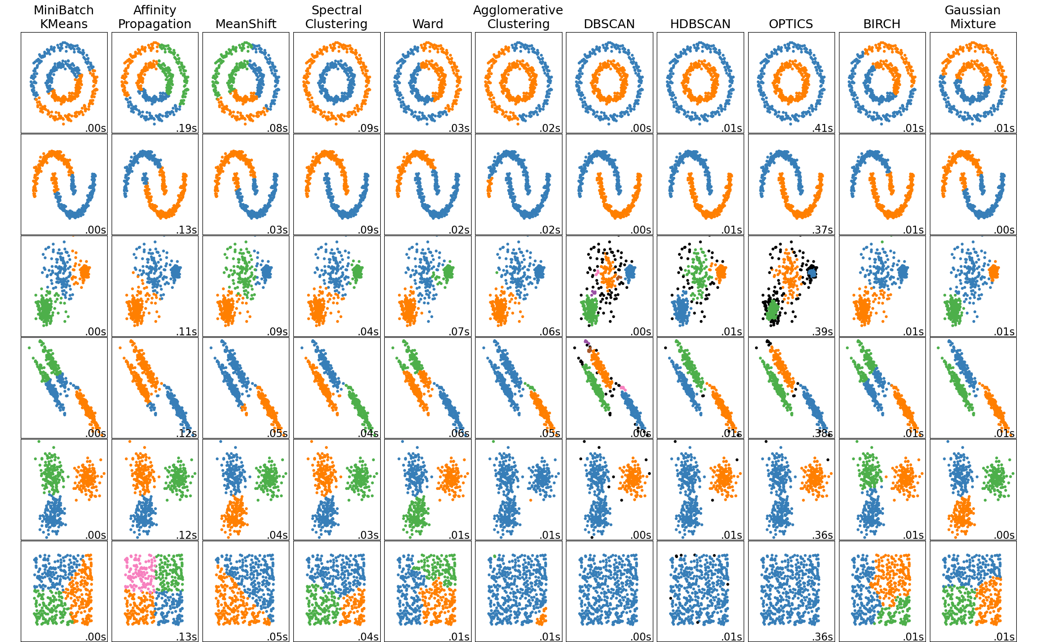
Types of Clustering Algorithms
- Connectivity-based (hierarchical)
- Centroid-based (k-means, k-medoid, c-means, etc.)
- Distribution-based (clusters are groups most likely belonging to the same distribution)
- Density-based (DBSCAN)
- Grid-based
In [1]:
import pandas as pd
import geopandas as gpd
from esda.moran import Moran
from libpysal.weights import Queen, KNN
import numpy as np
import matplotlib.pyplot as plt
import seaborn as sns
import pingouin as pg
C:\Users\barguzin\Anaconda3\envs\geo_env\lib\site-packages\outdated\utils.py:14: OutdatedPackageWarning: The package outdated is out of date. Your version is 0.2.1, the latest is 0.2.2.
Set the environment variable OUTDATED_IGNORE=1 to disable these warnings.
  return warn(
Using PySAL example data
In [2]:
from libpysal.examples import load_example, available

#[_ for _ in available().Name]

cin = load_example('Cincinnati')
cin.get_file_list()
Example not available: Cincinnati
Example not downloaded: Chicago parcels
Example not downloaded: Chile Migration
Example not downloaded: Spirals
Out[2]:
['C:\\Users\\barguzin\\pysal_data\\Cincinnati\\walnuthills_updated\\.DS_Store',
 'C:\\Users\\barguzin\\pysal_data\\Cincinnati\\walnuthills_updated\\cincinnati.dbf',
 'C:\\Users\\barguzin\\pysal_data\\Cincinnati\\walnuthills_updated\\cincinnati.prj',
 'C:\\Users\\barguzin\\pysal_data\\Cincinnati\\walnuthills_updated\\cincinnati.shp',
 'C:\\Users\\barguzin\\pysal_data\\Cincinnati\\walnuthills_updated\\cincinnati.shx',
 'C:\\Users\\barguzin\\pysal_data\\Cincinnati\\__MACOSX\\walnuthills_updated\\._.DS_Store']
In [3]:
cin_df = gpd.read_file(cin.get_path('cincinnati.shp'))
print(cin_df.shape)
cin_df.head()
(457, 73)
Out[3]:
| ID | AREA | BLOCK | BG | TRACT | COUNTY | MSA | POPULATION | MALE | FEMALE | ... | OWNER_SIZE | RENTER_SIZ | DENSITY | BURGLARY | ASSAULT | THEFT | BURG_D | ASSALT_D | THEFT_D | geometry | |
|---|---|---|---|---|---|---|---|---|---|---|---|---|---|---|---|---|---|---|---|---|---|
| 0 | 726907.0 | 0.09 | 390610042002001 | 390610042002 | 39061004200 | 39061 | 1640 | 479.0 | 221.0 | 258.0 | ... | 1.46 | 1.42 | 5384.7901 | 1 | 0 | 4 | 1.0 | 0.0 | 1.0 | POLYGON ((1407302.966 415693.734, 1407473.141 ... |
| 1 | 695744.0 | 0.01 | 390610022004003 | 390610022004 | 39061002200 | 39061 | 1640 | 85.0 | 39.0 | 46.0 | ... | 3.22 | 2.15 | 6643.1423 | 0 | 2 | 2 | 0.0 | 1.0 | 1.0 | POLYGON ((1398841.243 416718.444, 1399605.382 ... |
| 2 | 695762.0 | 0.01 | 390610033002017 | 390610033002 | 39061003300 | 39061 | 1640 | 29.0 | 18.0 | 11.0 | ... | 1.00 | 1.33 | 4326.5018 | 0 | 0 | 0 | 0.0 | 0.0 | 0.0 | POLYGON ((1398733.468 416975.853, 1398794.240 ... |
| 3 | 695780.0 | 0.01 | 390610022004002 | 390610022004 | 39061002200 | 39061 | 1640 | 117.0 | 59.0 | 58.0 | ... | 2.57 | 2.25 | 20784.6991 | 2 | 3 | 4 | 1.0 | 1.0 | 1.0 | POLYGON ((1399564.078 416046.633, 1399605.382 ... |
| 4 | 695798.0 | 0.02 | 390610033001009 | 390610033001 | 39061003300 | 39061 | 1640 | 96.0 | 51.0 | 45.0 | ... | 1.00 | 1.42 | 4019.0506 | 0 | 0 | 2 | 0.0 | 0.0 | 1.0 | POLYGON ((1398841.243 416718.444, 1398733.468 ... |
5 rows × 73 columns
In [4]:
cin_df[['WHITE', 'AP_WHITE']].describe()
Out[4]:
| WHITE | AP_WHITE | |
|---|---|---|
| count | 457.000000 | 457.000000 |
| mean | 23.954048 | 24.870897 |
| std | 65.200837 | 66.990628 |
| min | 0.000000 | 0.000000 |
| 25% | 0.000000 | 0.000000 |
| 50% | 3.000000 | 4.000000 |
| 75% | 19.000000 | 21.000000 |
| max | 634.000000 | 657.000000 |
In [5]:
cin_df[['OCCHU_OWNE', 'OCCHU_RENT']].describe()
Out[5]:
| OCCHU_OWNE | OCCHU_RENT | |
|---|---|---|
| count | 457.000000 | 457.000000 |
| mean | 8.617068 | 28.070022 |
| std | 18.680250 | 46.020203 |
| min | 0.000000 | 0.000000 |
| 25% | 0.000000 | 1.000000 |
| 50% | 4.000000 | 14.000000 |
| 75% | 10.000000 | 35.000000 |
| max | 245.000000 | 543.000000 |
In [6]:
cin_df.plot()
Out[6]:
<AxesSubplot:>

In [7]:
cin_df.info()
<class 'geopandas.geodataframe.GeoDataFrame'>
RangeIndex: 457 entries, 0 to 456
Data columns (total 73 columns):
 #   Column      Non-Null Count  Dtype
---  ------      --------------  -----
 0   ID          457 non-null    float64
 1   AREA        457 non-null    float64
 2   BLOCK       457 non-null    object
 3   BG          457 non-null    object
 4   TRACT       457 non-null    object
 5   COUNTY      457 non-null    object
 6   MSA         457 non-null    object
 7   POPULATION  457 non-null    float64
 8   MALE        457 non-null    float64
 9   FEMALE      457 non-null    float64
 10  AGE_0_5     457 non-null    float64
 11  AGE_5_9     457 non-null    float64
 12  AGE_10_14   457 non-null    float64
 13  AGE_15_19   457 non-null    float64
 14  AGE_20_24   457 non-null    float64
 15  AGE_25_34   457 non-null    float64
 16  AGE_35_44   457 non-null    float64
 17  AGE_45_54   457 non-null    float64
 18  AGE_55_59   457 non-null    float64
 19  AGE_60_64   457 non-null    float64
 20  AGE_65_74   457 non-null    float64
 21  AGE_75_84   457 non-null    float64
 22  AGE_85      457 non-null    float64
 23  MEDIAN_AGE  457 non-null    float64
 24  AGE_18      457 non-null    float64
 25  MALE_18     457 non-null    float64
 26  FEMALE_18   457 non-null    float64
 27  AGE_21      457 non-null    float64
 28  AGE_62      457 non-null    float64
 29  AGE_65      457 non-null    float64
 30  MALE_65     457 non-null    float64
 31  FEMALE_65   457 non-null    float64
 32  F1_RACE     457 non-null    float64
 33  WHITE       457 non-null    float64
 34  BLACK       457 non-null    float64
 35  AMINDIAN    457 non-null    float64
 36  ASIAN       457 non-null    float64
 37  HAWAIIAN    457 non-null    float64
 38  OTHER_RACE  457 non-null    float64
 39  F2_RACES    457 non-null    float64
 40  AP_WHITE    457 non-null    float64
 41  AP_BLACK    457 non-null    float64
 42  AP_AMINDIA  457 non-null    float64
 43  AP_ASIAN    457 non-null    float64
 44  AP_HAWAIIA  457 non-null    float64
 45  AP_OTHER    457 non-null    float64
 46  AP_HISPANI  457 non-null    float64
 47  NOT_HISPAN  457 non-null    float64
 48  NH_WHITE    457 non-null    float64
 49  IN_HOUSEHO  457 non-null    float64
 50  GROUP_QUAR  457 non-null    float64
 51  GQ_INSTITU  457 non-null    float64
 52  GQ_NONINST  457 non-null    float64
 53  HOUSEHOLDS  457 non-null    float64
 54  HH_FAMILY   457 non-null    float64
 55  HH_NONFAMI  457 non-null    float64
 56  AVG_HHSIZE  457 non-null    float64
 57  AVG_FAMSIZ  457 non-null    float64
 58  HSNG_UNITS  457 non-null    float64
 59  HU_OCCUPIE  457 non-null    float64
 60  HU_VACANT   457 non-null    float64
 61  OCCHU_OWNE  457 non-null    float64
 62  OCCHU_RENT  457 non-null    float64
 63  OWNER_SIZE  457 non-null    float64
 64  RENTER_SIZ  457 non-null    float64
 65  DENSITY     457 non-null    float64
 66  BURGLARY    457 non-null    int64
 67  ASSAULT     457 non-null    int64
 68  THEFT       457 non-null    int64
 69  BURG_D      457 non-null    float64
 70  ASSALT_D    457 non-null    float64
 71  THEFT_D     457 non-null    float64
 72  geometry    457 non-null    geometry
dtypes: float64(64), geometry(1), int64(3), object(5)
memory usage: 260.8+ KB
In [8]:
# consider only specific variables for clustering
# see variable description at GEODA lab
# https://geodacenter.github.io/data-and-lab/walnut_hills/
predictors = ['POPULATION', 'MEDIAN_AGE', 'AGE_65', 'WHITE', 'BLACK', 'ASIAN',
          'NH_WHITE', 'HOUSEHOLDS', 'AVG_HHSIZE', 'HU_VACANT', 'OCCHU_OWNE', 'OCCHU_RENT']

crime_vars = ['BURGLARY', 'ASSAULT', 'THEFT']

# more examples with plotting available from
# https://geographicdata.science/book/notebooks/10_clustering_and_regionalization.html
In [9]:
f, axs = plt.subplots(nrows=3, ncols=4, figsize=(16, 12))
# Make the axes accessible with single indexing
axs = axs.flatten()
# Start a loop over all the variables of interest
for i, col in enumerate(predictors):
    # select the axis where the map will go
    ax = axs[i]
    # Plot the map
    cin_df.plot(
        column=col,
        ax=ax,
        scheme="Quantiles",
        linewidth=0,
        cmap="BuPu",
    )
    # Remove axis clutter
    ax.set_axis_off()
    # Set the axis title to the name of variable being plotted
    ax.set_title(col)

f.savefig('crime_predictors.png')
plt.close()
C:\Users\barguzin\Anaconda3\envs\geo_env\lib\site-packages\mapclassify\classifiers.py:238: UserWarning: Warning: Not enough unique values in array to form k classes
  Warn(
C:\Users\barguzin\Anaconda3\envs\geo_env\lib\site-packages\mapclassify\classifiers.py:241: UserWarning: Warning: setting k to 3
  Warn("Warning: setting k to %d" % k_q, UserWarning)
In [10]:
from IPython.display import Image
Image(filename='crime_predictors.png')
Out[10]:

In [11]:
f, axs = plt.subplots(nrows=1, ncols=3, figsize=(16, 4))
# Make the axes accessible with single indexing
axs = axs.flatten()
# Start a loop over all the variables of interest
for i, col in enumerate(crime_vars):
    # select the axis where the map will go
    ax = axs[i]
    # Plot the map
    cin_df.plot(
        column=col,
        ax=ax,
        scheme="Quantiles",
        linewidth=0,
        cmap="BuPu",
    )
    # Remove axis clutter
    ax.set_axis_off()
    # Set the axis title to the name of variable being plotted
    ax.set_title(col)

f.savefig('crime_types.png')
plt.close()
C:\Users\barguzin\Anaconda3\envs\geo_env\lib\site-packages\mapclassify\classifiers.py:238: UserWarning: Warning: Not enough unique values in array to form k classes
  Warn(
C:\Users\barguzin\Anaconda3\envs\geo_env\lib\site-packages\mapclassify\classifiers.py:241: UserWarning: Warning: setting k to 3
  Warn("Warning: setting k to %d" % k_q, UserWarning)
C:\Users\barguzin\Anaconda3\envs\geo_env\lib\site-packages\mapclassify\classifiers.py:238: UserWarning: Warning: Not enough unique values in array to form k classes
  Warn(
C:\Users\barguzin\Anaconda3\envs\geo_env\lib\site-packages\mapclassify\classifiers.py:241: UserWarning: Warning: setting k to 4
  Warn("Warning: setting k to %d" % k_q, UserWarning)
In [12]:
from IPython.display import Image
Image(filename='crime_types.png')
Out[12]:

In [13]:
w = Queen.from_dataframe(cin_df)

# Calculate Moran's I for each variable
mi_results = [
    Moran(cin_df[variable], w) for variable in predictors
]
# Structure results as a list of tuples
mi_results = [
    (variable, res.I, res.p_sim)
    for variable, res in zip(predictors, mi_results)
]
# Display on table
table = pd.DataFrame(
    mi_results, columns=["Variable", "Moran's I", "P-value"]
).set_index("Variable")
table
C:\Users\barguzin\Anaconda3\envs\geo_env\lib\site-packages\libpysal\weights\_contW_lists.py:29: ShapelyDeprecationWarning: Iteration over multi-part geometries is deprecated and will be removed in Shapely 2.0. Use the `geoms` property to access the constituent parts of a multi-part geometry.
  return list(it.chain(*(list(zip(*shape.coords.xy)) for shape in shape)))
Out[13]:
| Moran's I | P-value | |
|---|---|---|
| Variable | ||
| POPULATION | 0.162529 | 0.001 |
| MEDIAN_AGE | 0.175654 | 0.001 |
| AGE_65 | 0.127756 | 0.002 |
| WHITE | 0.264340 | 0.001 |
| BLACK | 0.285679 | 0.001 |
| ASIAN | 0.057050 | 0.011 |
| NH_WHITE | 0.263554 | 0.001 |
| HOUSEHOLDS | 0.165267 | 0.001 |
| AVG_HHSIZE | 0.284141 | 0.001 |
| HU_VACANT | 0.198203 | 0.001 |
| OCCHU_OWNE | 0.245055 | 0.001 |
| OCCHU_RENT | 0.133238 | 0.001 |
Each of the variables displays significant positive spatial autocorrelation, suggesting clear spatial structure in the socioeconomic geography of San Diego. This means it is likely the clusters we find will have a non random spatial distribution.
In [14]:
xy_vars = predictors + ['BURGLARY']

corr_df = pg.pairwise_corr(cin_df[xy_vars], method='pearson')
corr_df.loc[corr_df.Y == 'BURGLARY'].sort_values(by='r', ascending=False)
Out[14]:
| X | Y | method | alternative | n | r | CI95% | p-unc | BF10 | power | |
|---|---|---|---|---|---|---|---|---|---|---|
| 67 | HOUSEHOLDS | BURGLARY | pearson | two-sided | 457 | 0.550126 | [0.48, 0.61] | 1.647029e-37 | 1.683e+34 | 1.000000 |
| 77 | OCCHU_RENT | BURGLARY | pearson | two-sided | 457 | 0.541269 | [0.47, 0.6] | 3.835054e-36 | 7.444e+32 | 1.000000 |
| 11 | POPULATION | BURGLARY | pearson | two-sided | 457 | 0.499936 | [0.43, 0.57] | 2.856307e-30 | 1.146e+27 | 1.000000 |
| 74 | HU_VACANT | BURGLARY | pearson | two-sided | 457 | 0.499887 | [0.43, 0.57] | 2.899383e-30 | 1.129e+27 | 1.000000 |
| 49 | BLACK | BURGLARY | pearson | two-sided | 457 | 0.492950 | [0.42, 0.56] | 2.351419e-29 | 1.424e+26 | 1.000000 |
| 76 | OCCHU_OWNE | BURGLARY | pearson | two-sided | 457 | 0.385024 | [0.3, 0.46] | 1.344824e-17 | 3.565e+14 | 1.000000 |
| 32 | AGE_65 | BURGLARY | pearson | two-sided | 457 | 0.377739 | [0.3, 0.45] | 6.014186e-17 | 8.173e+13 | 1.000000 |
| 62 | NH_WHITE | BURGLARY | pearson | two-sided | 457 | 0.240948 | [0.15, 0.33] | 1.850323e-07 | 4.481e+04 | 0.999485 |
| 41 | WHITE | BURGLARY | pearson | two-sided | 457 | 0.239724 | [0.15, 0.32] | 2.142888e-07 | 3.89e+04 | 0.999432 |
| 71 | AVG_HHSIZE | BURGLARY | pearson | two-sided | 457 | 0.144546 | [0.05, 0.23] | 1.949163e-03 | 6.998 | 0.873839 |
| 22 | MEDIAN_AGE | BURGLARY | pearson | two-sided | 457 | 0.115112 | [0.02, 0.2] | 1.380667e-02 | 1.202 | 0.693597 |
| 56 | ASIAN | BURGLARY | pearson | two-sided | 457 | 0.035869 | [-0.06, 0.13] | 4.443094e-01 | 0.078 | 0.119285 |
Similarity
- Absolute values will drown variables which have higher range of values (0-1 Vs 0-1000)
- Standardize values by mean and stdev
- For non-normal, skewed and bimodal distributions robust scaling may be required!
- Use sklearn package
Standardizing Variables
- scale(): $z = \frac{x_i - \bar{x}}{\sigma_x}$
- robust_scale(): $z = \frac{x_i - \tilde{x}}{\lceil x \rceil_{75} - \lceil x \rceil_{25}}$ (median and IQR)
- minmax_scale(): $z = \frac{x - min(x)}{max(x-min(x))}$
In [15]:
from sklearn.preprocessing import robust_scale

db_scaled = robust_scale(cin_df[predictors])
K-means Clustering
- Pre-specified number of clusters (groups)
- Each observation is closer to the mean of its own group than it is to the mean of any other group
K-means Clustering Algorithm
- Assign all observations to one of the $k$ labels
- Calculate multivariate mean over all covaraites for each cluster
- Reassign observations to the cluster with closest mean
- Repeat and update until there are no more changes
In [16]:
# Initialise KMeans instance
from sklearn.cluster import KMeans
# Initialise KMeans instance
kmeans = KMeans(n_clusters=5)
# Set the seed for reproducibility
np.random.seed(1234)
# Run K-Means algorithm
k5cls = kmeans.fit(db_scaled)
# Print first five labels
k5cls.labels_[:5]
C:\Users\barguzin\Anaconda3\envs\geo_env\lib\site-packages\sklearn\cluster\_kmeans.py:1334: UserWarning: KMeans is known to have a memory leak on Windows with MKL, when there are less chunks than available threads. You can avoid it by setting the environment variable OMP_NUM_THREADS=2.
  warnings.warn(
Out[16]:
array([3, 0, 0, 0, 0])
In [17]:
# Assign labels into a column
cin_df["k5cls"] = k5cls.labels_
# Setup figure and ax
f, ax = plt.subplots(1, figsize=(9, 9))
# Plot unique values choropleth including
# a legend and with no boundary lines
cin_df.plot(
    column="k5cls", categorical=True, legend=True, linewidth=0, ax=ax
)
# Remove axis
ax.set_axis_off()
f.savefig('kmeans.png')
plt.close()
In [18]:
Image(filename='kmeans.png')
Out[18]:

Characterizing Clusters
- Very imbalanced partitioning
- Some contiguity is noticeable, but the arrangement is patchy
In [19]:
# Group data table by cluster label and count observations
k5sizes = cin_df.groupby("k5cls").size()
k5sizes
Out[19]:
k5cls
0    417
1      1
2      1
3     10
4     28
dtype: int64
In [20]:
# Dissolve areas by Cluster, aggregate by summing,
# and keep column for area
areas = cin_df.dissolve(by="k5cls", aggfunc="sum")['geometry'].area
areas
Out[20]:
k5cls
0    9.993732e+07
1    1.116340e+06
2    6.673713e+05
3    1.572282e+07
4    3.126180e+07
dtype: float64
In [21]:
# Group table by cluster label, keep the variables used
# for clustering, and obtain their mean
k5means = cin_df.groupby("k5cls")[predictors].mean()
# Transpose the table and print it rounding each value
# to three decimals
k5means.T.round(3)
Out[21]:
| k5cls | 0 | 1 | 2 | 3 | 4 |
|---|---|---|---|---|---|
| POPULATION | 56.942 | 1108.00 | 361.00 | 420.400 | 331.893 |
| MEDIAN_AGE | 26.170 | 21.80 | 25.00 | 29.310 | 41.879 |
| AGE_65 | 4.851 | 6.00 | 16.00 | 35.400 | 72.179 |
| WHITE | 13.084 | 435.00 | 259.00 | 325.000 | 55.250 |
| BLACK | 41.806 | 244.00 | 5.00 | 61.300 | 268.821 |
| ASIAN | 0.518 | 372.00 | 85.00 | 21.900 | 1.250 |
| NH_WHITE | 12.926 | 422.00 | 258.00 | 322.300 | 54.464 |
| HOUSEHOLDS | 24.890 | 356.00 | 180.00 | 139.500 | 159.143 |
| AVG_HHSIZE | 1.830 | 1.92 | 1.87 | 1.548 | 1.915 |
| HU_VACANT | 5.309 | 6.00 | 13.00 | 17.900 | 22.393 |
| OCCHU_OWNE | 5.746 | 2.00 | 29.00 | 45.000 | 37.893 |
| OCCHU_RENT | 19.144 | 354.00 | 151.00 | 94.500 | 121.250 |
In [22]:
# Index db on cluster ID
tidy_db = cin_df.set_index("k5cls")
# Keep only variables used for clustering
tidy_db = tidy_db[predictors]
# Stack column names into a column, obtaining
# a "long" version of the dataset
tidy_db = tidy_db.stack()
# Take indices into proper columns
tidy_db = tidy_db.reset_index()
# Rename column names
tidy_db = tidy_db.rename(
    columns={"level_1": "Attribute", 0: "Values"}
)
# Check out result
tidy_db.head()
Out[22]:
| k5cls | Attribute | Values | |
|---|---|---|---|
| 0 | 3 | POPULATION | 479.0 |
| 1 | 3 | MEDIAN_AGE | 55.7 |
| 2 | 3 | AGE_65 | 174.0 |
| 3 | 3 | WHITE | 433.0 |
| 4 | 3 | BLACK | 32.0 |
In [23]:
# Scale fonts to make them more readable
sns.set(font_scale=1.5)
# Setup the facets
facets = sns.FacetGrid(
    data=tidy_db,
    col="Attribute",
    hue="k5cls",
    sharey=False,
    sharex=False,
    aspect=2,
    col_wrap=3
)
# Build the plot from `sns.kdeplot`
_ = facets.map(sns.kdeplot, "Values", fill=True, warn_singular=False).add_legend()

Hierarchical Clustering
- Agglomerative Hierarchical Clustering (AHC)
- Hierarchy of solutions (starts at singletons) and assign all observations into same cluster
- We are looking for in-between clustering solutions
AHC Algorithm
- Every observation is its own cluster
- Find two closest observations based on distance metric (Euclidean Distance)
- Join the closest into a new cluster
- Repeat 2 and 3 until reaching the desired degree of aggregation
In [24]:
from sklearn.cluster import AgglomerativeClustering

# Set seed for reproducibility
np.random.seed(0)
# Iniciate the algorithm
model = AgglomerativeClustering(linkage="ward", n_clusters=5)
# Run clustering
model.fit(db_scaled)
# Assign labels to main data table
cin_df["ward5"] = model.labels_
In [25]:
ward5sizes = cin_df.groupby("ward5").size()
ward5sizes
Out[25]:
ward5
0    442
1      5
2      8
3      1
4      1
dtype: int64
In [26]:
ward5means = cin_df.groupby("ward5")[predictors].mean()
ward5means.T.round(3)
Out[26]:
| ward5 | 0 | 1 | 2 | 3 | 4 |
|---|---|---|---|---|---|
| POPULATION | 70.152 | 583.600 | 414.625 | 1108.00 | 361.00 |
| MEDIAN_AGE | 26.969 | 52.520 | 24.462 | 21.80 | 25.00 |
| AGE_65 | 7.964 | 154.600 | 13.125 | 6.00 | 16.00 |
| WHITE | 14.760 | 244.400 | 313.375 | 435.00 | 259.00 |
| BLACK | 53.041 | 324.200 | 63.500 | 244.00 | 5.00 |
| ASIAN | 0.550 | 5.000 | 25.250 | 372.00 | 85.00 |
| NH_WHITE | 14.566 | 242.200 | 311.125 | 422.00 | 258.00 |
| HOUSEHOLDS | 31.260 | 317.200 | 103.375 | 356.00 | 180.00 |
| AVG_HHSIZE | 1.835 | 1.688 | 1.557 | 1.92 | 1.87 |
| HU_VACANT | 6.163 | 38.400 | 13.000 | 6.00 | 13.00 |
| OCCHU_OWNE | 7.165 | 125.000 | 14.375 | 2.00 | 29.00 |
| OCCHU_RENT | 24.095 | 192.200 | 89.000 | 354.00 | 151.00 |
In [27]:
# Index db on cluster ID
tidy_db = cin_df.set_index("ward5")
# Keep only variables used for clustering
tidy_db = tidy_db[predictors]
# Stack column names into a column, obtaining
# a "long" version of the dataset
tidy_db = tidy_db.stack()
# Take indices into proper columns
tidy_db = tidy_db.reset_index()
# Rename column names
tidy_db = tidy_db.rename(
    columns={"level_1": "Attribute", 0: "Values"}
)
# Check out result
tidy_db.head()
Out[27]:
| ward5 | Attribute | Values | |
|---|---|---|---|
| 0 | 1 | POPULATION | 479.0 |
| 1 | 1 | MEDIAN_AGE | 55.7 |
| 2 | 1 | AGE_65 | 174.0 |
| 3 | 1 | WHITE | 433.0 |
| 4 | 1 | BLACK | 32.0 |
In [28]:
# Setup the facets
facets = sns.FacetGrid(
    data=tidy_db,
    col="Attribute",
    hue="ward5",
    sharey=False,
    sharex=False,
    aspect=2,
    col_wrap=3,
)
# Build the plot as a `sns.kdeplot`
facets.map(sns.kdeplot, "Values", fill=True, warn_singular=False).add_legend()
Out[28]:
<seaborn.axisgrid.FacetGrid at 0x212a852c7f0>

In [29]:
# Setup figure and ax
f, axs = plt.subplots(1, 2, figsize=(12, 6))

### K-Means ###
ax = axs[0]
# Plot unique values choropleth including
# a legend and with no boundary lines
cin_df.plot(
    column="k5cls",
    categorical=True,
    cmap="Set2",
    legend=True,
    linewidth=0,
    ax=ax,
)
# Remove axis
ax.set_axis_off()
# Add title
ax.set_title("K-Means solution ($k=5$)")

### AHC ###
ax = axs[1]
# Plot unique values choropleth including
# a legend and with no boundary lines
cin_df.plot(
    column="ward5",
    categorical=True,
    cmap="Set3",
    legend=True,
    linewidth=0,
    ax=ax,
)
# Remove axis
ax.set_axis_off()
# Add title
ax.set_title("AHC solution ($k=5$)")

# Display the map
f.savefig('two_clust.png')
plt.close()
In [30]:
Image(filename='two_clust.png')
Out[30]:

Why Regionalization
- Clustering helps us investigate the structure of our data (spatial contiguity is not always a requirement)
- We impose spatial constraint on clusters (geographically coherent areas + coherent data profiles)
- Counties within states (administrative principles), clusters within out data (statistical similarity)
- Spatial weights matrix can be used as a measure of spatial similarity
In [31]:
# Set the seed for reproducibility
np.random.seed(123456)
# Specify cluster model with spatial constraint
regi = AgglomerativeClustering(
    linkage="ward", connectivity=w.sparse, n_clusters=5
)
# Fit algorithm to the data
regi.fit(db_scaled)
Out[31]:
AgglomerativeClustering(connectivity=<457x457 sparse matrix of type '<class 'numpy.float64'>'
	with 2970 stored elements in Compressed Sparse Row format>,
                        n_clusters=5)
In a Jupyter environment, please rerun this cell to show the HTML representation or trust the notebook. On GitHub, the HTML representation is unable to render, please try loading this page with nbviewer.org.
AgglomerativeClustering(connectivity=<457x457 sparse matrix of type '<class 'numpy.float64'>'
	with 2970 stored elements in Compressed Sparse Row format>,
                        n_clusters=5)
In [32]:
cin_df["ward5wq"] = regi.labels_
# Setup figure and ax
f, ax = plt.subplots(1, figsize=(5, 5))
# Plot unique values choropleth including a legend and with no boundary lines
cin_df.plot(
    column="ward5wq",
    categorical=True,
    legend=True,
    linewidth=0,
    ax=ax,
)
# Remove axis
ax.set_axis_off()
# Display the map
plt.show()

Why are we getting imbalanced clusters?
- Data is not normal
- Methods are not robust to outliers
In [33]:
cin_df[predictors].plot.hist(subplots=True, legend=True, layout=(4,3), figsize=(16,12), sharex=False);

K-Medoids Clustering (PAM)
- Partitioning around medoid (instead of 'mean', select most central actual observation).
- The medoid of a cluster is defined as the object in the cluster whose average dissimilarity to all the objects in the cluster is minimal, that is, it is a most centrally located point in the cluster.
- $k$-medoids minimizes a sum of pairwise dissimilarities instead of a sum of squared Euclidean distances (depends on implementation), it is more robust to noise and outliers than k-means
In [34]:
from sklearn_extra.cluster import KMedoids

kmedoids = KMedoids(n_clusters=5, random_state=0)

medo = kmedoids.fit(db_scaled)
In [35]:
cin_df["medo_k5"] = medo.labels_
# Setup figure and ax
f, ax = plt.subplots(1, figsize=(5, 5))
# Plot unique values choropleth including a legend and with no boundary lines
cin_df.plot(
    column="medo_k5",
    categorical=True,
    legend=True,
    linewidth=0,
    ax=ax,
)
# Remove axis
ax.set_axis_off()
# Display the map
plt.show()

Feature Engineering
- Get $X$ and $Y$ coordinates from block centroids
- Normalize absolute values into percentage points
- pct_elder
- pct_white
- pct_black
- pct_own
- pct_rent
- pct_vac
- fill missing values with zeroes (for any gaps in our data)
In [36]:
# add xy to clustering
cin_df2 = cin_df.copy()

# calculate centroid locs
cin_df2['lng'] = cin_df2.centroid.x
cin_df2['lat'] = cin_df2.centroid.y

# pct vars
cin_df2['pct_elder']  = cin_df2.AGE_65 / cin_df2.POPULATION
cin_df2['pct_white']  = cin_df2.WHITE / cin_df2.POPULATION
cin_df2['pct_black']  = cin_df2.BLACK / cin_df2.POPULATION
cin_df2['pct_own'] = cin_df2.OCCHU_OWNE / cin_df2.HSNG_UNITS
cin_df2['pct_rent'] = cin_df2.OCCHU_RENT / cin_df2.HSNG_UNITS
cin_df2['pct_vac'] = cin_df2.HU_VACANT / cin_df2.HSNG_UNITS

cin_df2 = cin_df2.fillna(0)

new_predictors = ['POPULATION', 'MEDIAN_AGE', 'lng', 'lat', 'pct_elder', 'pct_white', 'pct_black',
                 'pct_own', 'pct_rent', 'pct_vac']
In [37]:
db_scaled2 = robust_scale(cin_df2[new_predictors])
In [38]:
# Set the seed for reproducibility
np.random.seed(123456)
# Specify cluster model with spatial constraint
xy_norm_model = AgglomerativeClustering(
    linkage="ward",
    #connectivity=w.sparse,
    n_clusters=5
)
# Fit algorithm to the data
xy_norm_model.fit(db_scaled2)
Out[38]:
AgglomerativeClustering(n_clusters=5)In a Jupyter environment, please rerun this cell to show the HTML representation or trust the notebook.
On GitHub, the HTML representation is unable to render, please try loading this page with nbviewer.org.
AgglomerativeClustering(n_clusters=5)
In [39]:
cin_df2["xy_norm_model"] = xy_norm_model.labels_
# Setup figure and ax
f, ax = plt.subplots(1, figsize=(5, 5))
# Plot unique values choropleth including a legend and with no boundary lines
cin_df2.plot(
    column="xy_norm_model",
    categorical=True,
    legend=True,
    linewidth=0,
    ax=ax,
)
# Remove axis
ax.set_axis_off()
# Display the map
plt.show()

In [40]:
# Set the seed for reproducibility
np.random.seed(123456)
# Specify cluster model with spatial constraint
xy_norm_geo_model = AgglomerativeClustering(
    linkage="ward",
    connectivity=w.sparse,
    n_clusters=5
)
# Fit algorithm to the data
xy_norm_geo_model.fit(db_scaled2)
Out[40]:
AgglomerativeClustering(connectivity=<457x457 sparse matrix of type '<class 'numpy.float64'>'
	with 2970 stored elements in Compressed Sparse Row format>,
                        n_clusters=5)
In a Jupyter environment, please rerun this cell to show the HTML representation or trust the notebook. On GitHub, the HTML representation is unable to render, please try loading this page with nbviewer.org.
AgglomerativeClustering(connectivity=<457x457 sparse matrix of type '<class 'numpy.float64'>'
	with 2970 stored elements in Compressed Sparse Row format>,
                        n_clusters=5)
In [41]:
cin_df2["xy_norm_geo5"] = xy_norm_geo_model.labels_
# Setup figure and ax
f, ax = plt.subplots(1, figsize=(5, 5))
# Plot unique values choropleth including a legend and with no boundary lines
cin_df2.plot(
    column="xy_norm_geo5",
    categorical=True,
    legend=True,
    linewidth=0,
    ax=ax,
)
# Remove axis
ax.set_axis_off()
# Display the map
plt.show()

The Final View of Partitioning for Data
In [42]:
sns.set(font_scale=1)
fig, axs = plt.subplots(3, 2, figsize=(10, 16))

axs = axs.flatten();

cin_df2.plot(column="k5cls", categorical=True, legend=True, linewidth=0, ax=axs[0]);
axs[0].set_title('k-Means Clustering (k=5)', fontsize=14);

cin_df2.plot(column="ward5", categorical=True, legend=True, linewidth=0, ax=axs[1]);
axs[1].set_title('AHC Clustering (k=5)', fontsize=14);

cin_df2.plot(column="ward5wq", categorical=True, legend=True, linewidth=0, ax=axs[2]);
axs[2].set_title('Regionalized AHC Clustering (k=5)', fontsize=14);

cin_df2.plot(column="medo_k5", categorical=True, legend=True, linewidth=0, ax=axs[3]);
axs[3].set_title('k-Medoids Clustering (k=5)', fontsize=14);

cin_df2.plot(column="xy_norm_model", categorical=True, legend=True, linewidth=0, ax=axs[4]);
axs[4].set_title('AHC Clustering with Normalized Variables \n and Geographic Coordinates  (k=5)', fontsize=14);

cin_df2.plot(column="xy_norm_geo5", categorical=True, legend=True, linewidth=0, ax=axs[5]);
axs[5].set_title('AHC Clustering with Normalized Variables \n and Geographic Coordinates and Contiguity  (k=5)', fontsize=14);

[i.set_axis_off() for i in axs]
plt.subplots_adjust(hspace=-0.45)
fig.savefig('all_clust.png', bbox_inches='tight')
plt.close()
In [43]:
Image(filename='all_clust.png')
Out[43]:
