GEOG 172: INTERMEDIATE GEOGRAPHICAL ANALYSIS

Evgeny Noi

Lecture 15: Linear Regression

Correction

The optimal number of clusters on this plot is 3! (The closer to +1 the better).

Announcements

• No labs this week (STRIKE)
• Extended office hours (M:2-6pm, W:1-3pm)
• Interim report due W: midnight

Correlation Refresher

• Correlation - is linear relationship between two variables (bivariate).
• Standardized measure (+1 / -1)
• Slope of the line between scatter points on a scatter plot

Different Ways to Understand Regression

• Fancy correlation
• Optimization problem
• statistical framework for modeling

!python -m wget https://geographicdata.science/book/_downloads/dcd429d1761a2d0efdbc4532e141ba14/regression_db.geojson

Saved under regression_db.geojson

import pandas as pd
import geopandas as gpd
import matplotlib.pyplot as plt 
import seaborn as sns
import pingouin as pg

db = gpd.read_file("regression_db.geojson")
print(db.shape) 
db.head()

(6110, 20)

	accommodates	bathrooms	bedrooms	beds	neighborhood	pool	d2balboa	coastal	price	log_price	id	pg_Apartment	pg_Condominium	pg_House	pg_Other	pg_Townhouse	rt_Entire_home/apt	rt_Private_room	rt_Shared_room	geometry
0	5	2.0	2.0	2.0	North Hills	0	2.972077	0	425.0	6.052089	6	0	0	1	0	0	1	0	0	POINT (-117.12971 32.75399)
1	6	1.0	2.0	4.0	Mission Bay	0	11.501385	1	205.0	5.323010	5570	0	1	0	0	0	1	0	0	POINT (-117.25253 32.78421)
2	2	1.0	1.0	1.0	North Hills	0	2.493893	0	99.0	4.595120	9553	1	0	0	0	0	0	1	0	POINT (-117.14121 32.75327)
3	2	1.0	1.0	1.0	Mira Mesa	0	22.293757	0	72.0	4.276666	14668	0	0	1	0	0	0	1	0	POINT (-117.15269 32.93110)
4	2	1.0	1.0	1.0	Roseville	0	6.829451	0	55.0	4.007333	38245	0	0	1	0	0	0	1	0	POINT (-117.21870 32.74202)

variable_names = [
    "accommodates",  # Number of people it accommodates
    "bathrooms",  # Number of bathrooms
    "bedrooms",  # Number of bedrooms
    "beds",  # Number of beds
    # Below are binary variables, 1 True, 0 False
    "rt_Private_room",  # Room type: private room
    "rt_Shared_room",  # Room type: shared room
    "pg_Condominium",  # Property group: condo
    "pg_House",  # Property group: house
    "pg_Other",  # Property group: other
    "pg_Townhouse",  # Property group: townhouse
]

How do we do analysis on this data?

1. Visualize
2. Run pairwise correlations
3. Run Global Moran's I (and local if necessary)
4. Run clustering (to investigate any patterns in multivariate data)
5. RUN REGRESSION (today)

fig, ax = plt.subplots(figsize=(7,7))
sns.heatmap(db.corr(), annot=True, ax=ax, 
            fmt=".1f", annot_kws={"size": 8}, 
           cmap='vlag', vmin=db.corr().min().min(), vmax=db.corr().max().max());
#plt.gcf().subplots_adjust(left=0.15)
fig.savefig('corr_matrix.png', bbox_inches='tight') 
plt.close()

from IPython.display import Image
Image(filename='corr_matrix.png') 

# now the same with the table 
db_corr = pg.pairwise_corr(db, method='pearson').sort_values(by='r')
db_corr.loc[(db_corr.X == 'log_price')|(db_corr.Y == 'log_price'), ['X', 'Y', 'r', 'p-unc']]

	X	Y	r	p-unc
115	log_price	rt_Private_room	-0.525523	0.000000e+00
116	log_price	rt_Shared_room	-0.277179	3.452531e-108
109	log_price	pg_Apartment	-0.140333	3.004493e-28
113	log_price	pg_Townhouse	0.005033	6.940470e-01
108	log_price	id	0.015802	2.168407e-01
65	pool	log_price	0.018576	1.465442e-01
112	log_price	pg_Other	0.031385	1.415184e-02
111	log_price	pg_House	0.073500	8.828480e-09
110	log_price	pg_Condominium	0.074952	4.469152e-09
77	d2balboa	log_price	0.132289	2.927701e-25
88	coastal	log_price	0.332528	1.165628e-157
52	beds	log_price	0.597273	0.000000e+00
23	bathrooms	log_price	0.605840	0.000000e+00
114	log_price	rt_Entire_home/apt	0.610318	0.000000e+00
38	bedrooms	log_price	0.670055	0.000000e+00
7	accommodates	log_price	0.727280	0.000000e+00
98	price	log_price	0.789370	0.000000e+00

fig, ax = plt.subplots() 
sns.scatterplot(data=db, x='log_price', y='accommodates', ax=ax, 
                hue='rt_Entire_home/apt', alpha=.5, s=15, 
               style='rt_Private_room');

fig, ax = plt.subplots() 
sns.regplot(data=db, x='log_price', y='accommodates', ax=ax);

Regression

Finding the best fitting line for the set of points (2d case) - GEOMETRIC SENSE!

Regression implies modeling dependent variable (outcome) using one or more independent variables (predictors)

The Modeling (statistical) Framework

• outcome - price of AirBnb in San Diego, predictors - # of bedrooms, bathrooms, type of property, etc.

We are trying to explain 'variance' in the outcome by 'variance' in predictors

Combining statistical + geometric framework

$$ \hat{Y_i} = b_0 + b_1 X_i + \epsilon_i $$

where $\hat{Y_i}$ denotes our prediction (line), $X_i$ predictor variable value for $i$th observations, $\beta_0$ is the intercept, and $\beta_1$ is the regression coefficient. And $\epsilon_i = \hat{Y_i} - Y_i$ (residuals/errors = predicted - actual values).

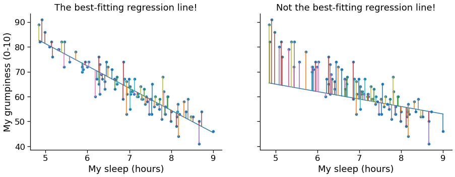
Geometry + Optimization

• We want our combined $\epsilon$ (error/residuals) to be as small as possible.

The estimated regression coefficients $\hat{\beta_0}$ and $\hat{\beta_1}$ are those that minimise the sum of the squared residuals

$$ \sum_i (Y_i - \hat{Y}_i)^2 $$

mod1 = pg.linear_regression(db['accommodates'], db['log_price'])
mod1

	names	coef	se	T	pval	r2	adj_r2	CI[2.5%]	CI[97.5%]
0	Intercept	4.123498	0.012696	324.794585	0.0	0.528936	0.528859	4.098610	4.148386
1	accommodates	0.206661	0.002495	82.815413	0.0	0.528936	0.528859	0.201769	0.211553

sns.scatterplot(data=db, x='price', y='log_price');

Understanding Regression Equation

$$ \hat{Y}_i = b_0 + b_1 X_i = 4.1 + 0.2 \ X_i $$

For 1-unit increase in the number of people that the Airbnb property accommodates, we expect the log(price) to go up by .2

The expected value of $\hat{Y_i}$ when $X_i = 0$ is 4.1

Caution ⚠️

Order in regression matters (typically, predictor goes first and outcome goes second)! We are modeling the log(price) as a function of the number of people that the apartment from the listing can accommodate.

Multiple Regression

• Adding terms to our equations (from bivariate to multivariate)

$$ Y_i = b_2 X_{i2} + b_1 X_{i1} + b_0 + \epsilon_i $$

mod2 = pg.linear_regression(db[['accommodates', 'bedrooms']], db['log_price'])
mod2.round(2)

	names	coef	se	T	pval	r2	adj_r2	CI[2.5%]	CI[97.5%]
0	Intercept	4.10	0.01	323.10	0.0	0.54	0.54	4.07	4.12
1	accommodates	0.16	0.00	35.33	0.0	0.54	0.54	0.15	0.17
2	bedrooms	0.15	0.01	13.44	0.0	0.54	0.54	0.13	0.17

Regression Equation

$$ \hat{Y}_i = 4.10 + 0.16 \ X_{i1} + 0.15 \ X_{i2} $$

Multivariate (general) Case

$$ Y_i = \left( \sum_{k=1}^K b_{k} X_{ik} \right) + b_0 + \epsilon_i $$

Quantifying the Fit of the Regression

$$ \mbox{SS}_{res} = \sum_i (Y_i - \hat{Y}_i)^2 \quad \text{sum of squared residuals} $$$$ \mbox{SS}_{tot} = \sum_i (Y_i - \bar{Y})^2 \quad \text{total variability} $$

# calculate 
Y_pred = mod1.loc[mod1.names=='Intercept','coef'].values + db['accommodates'] \
    * mod1.loc[mod1.names=='accommodates','coef'].values
Y_pred

0       5.156802
1       5.363463
2       4.536820
3       4.536820
4       4.536820
          ...   
6105    4.536820
6106    5.363463
6107    4.330159
6108    4.743481
6109    4.743481
Name: accommodates, Length: 6110, dtype: float64

SS_resid = sum( (db.log_price - Y_pred)**2 )
SS_tot = sum( (db.log_price - np.mean(db.log_price))**2 )
print(f'Squared residuals: {SS_resid}')
print(f'total variation: {SS_tot}')

Squared residuals: 1875.0601303913895
total variation: 3980.4790154915463

Making Fit Interpretable - R-squared

• Get standardized value (something similar to (auto)correlation coefficient)
• Make standardize value meaningful (good/bad) fit: +1 (good fit), 0 (no fit)

$$ R^2 = 1 - \frac{SS_{res}}{SS_{tot}} $$

R2 = 1- (SS_resid / SS_tot)
R2

0.5289360594305659

Interpreting R-squared

$R^2$ is the proportion of the variance in the outcome variable that can be accounted for by the predictor. The number of people accommodated per listing explains 52.9% of the variation in the price of the listing.

Adjusted R-squared

• Adding variables to the model will always increase $R^2$! BUT, we need to take degrees of freedom into account!
• The adjusted value will only increase if the new variables improve the model performance more than you’d expect by chance.
• We loose elegant interpretation about explained variability!

$$ \mbox{adj. } R^2 = 1 - \left(\frac{\mbox{SS}_{res}}{\mbox{SS}_{tot}} \times \frac{N-1}{N-K-1} \right) $$

where $N$ - is the number of observations, $K$ - number of predictors

Correlation and Regression Connection

$R^2$ is the same as $r_p$

Running regression with all predictors

from pysal.model import spreg

# Fit OLS model
m1 = spreg.OLS(
    # Dependent variable
    db[["log_price"]].values,
    # Independent variables
    db[variable_names].values,
    # Dependent variable name
    name_y="log_price",
    # Independent variable name
    name_x=variable_names,
)

with open('reg1.txt', 'w') as f:
    print(m1.summary, file=f)  # Python 3.x

print(m1.r2)
print(m1.ar2)

0.6683445024123358
0.667800715729949

Hypothesis Testing and Regression

• $H_0$: $H_0: Y_i = b_0 + \epsilon_i$ (there is no relationship)
• $H_a$: $H_1: Y_i = \left( \sum_{k=1}^K b_{k} X_{ik} \right) + b_0 + \epsilon_i$ (our proposed model is valid)

Hypothesis Testing (Calculation)

$$ \mbox{SS}_{mod} = \mbox{SS}_{tot} - \mbox{SS}_{res} $$$$ \begin{split} \begin{array}{rcl} \mbox{MS}_{mod} &=& \displaystyle\frac{\mbox{SS}_{mod} }{df_{mod}} \\ \\ \mbox{MS}_{res} &=& \displaystyle\frac{\mbox{SS}_{res} }{df_{res} } \end{array} \end{split} $$

where $df_{res} = N -K - 1$

Hypothesis Testing (Calculation)

$$ F = \frac{\mbox{MS}_{mod}}{\mbox{MS}_{res}} $$

Pingouin cannot calculate $F$ statistic. Instead we can use the summary table from spreg.

Other Hypothesis Tests (not covered in class)

• Test for individual coefficients
• Testing significance of correlation (both single and all pairwise)

See this tutorial for more details

Assumptions of the regression

• Normality. Standard linear regression relies on an assumption of normality. Specifically, it assumes that the residuals are normally distributed. It’s actually okay if the predictors and the outcome are non-normal, so long as the residuals are normal.
• Linearity. Relationship between $X$ and $Y$ are assumed linear! Regardless of whether it’s a simple regression or a multiple regression, we assume that the relatiships involved are linear.
• Homogeneity of variance. Each residual is generated from a normal distribution with mean 0, and with a standard deviation that is the same for every single residual. Standard deviation of the residual should be the same for all values of $\hat{Y_i}$.

Assumptions of the regression 2

• Uncorrelated predictors. We don’t want predictors to be too strongly correlated with each other. Predictors that are too strongly correlated with each other (referred to as “collinearity”) can cause problems when evaluating the model
• Residuals are independent of each other. Check residuals for irregularity in variance. Some irregularity would normally point to the omitted variable or OMITTED GEOGRAPHIC EFFECT!.
• Outliers. Implicit assumption that regression model should not be too strongly influenced by one or two anomalous data points; since this raises questions about the adequacy of the model, and the trustworthiness of the data in some cases.

Questions?