GEOG 172: INTERMEDIATE GEOGRAPHICAL ANALYSIS
Evgeny Noi
Lecture 18: Multi-scale Geographically Weighted Regression
Regression Modeling for Spatial Relations
- Spatial heterogeneity
- Fixed-effect model
- Spatial regimes
- Spatial Dependence
- SLX (spatial feature engineering)
- Spatial error model
- Spatial lag model
- Local Modeling Frameworks (GWR and MGWR)
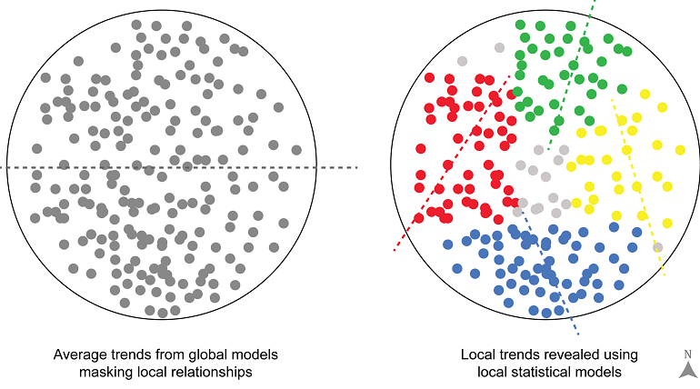
(M)GWR
- estimate location-dependent relationship between dependent and independent variables
- place-based analytic technique
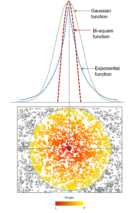
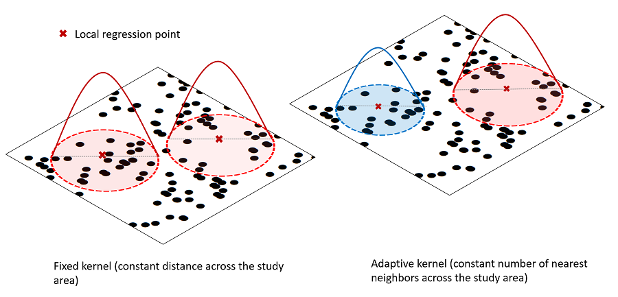
- GWR models borrow data from neighboring observations and weight these data according to a smooth decay function based on either a physical distance or the number of nearest neighbors (higher weight for nearby locations)
(M)GWR
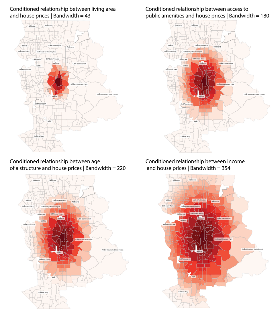
- Small bandwidths denote more local processes; large bandwidths indicate regional or global processes.
- As long as an optimal bandwidth is determined in the calibration of the GWR model and some continuous smooth function of distance is used, the specific kernel function chosen is not critical.
Selecting Optimal Bandwidth
- Trade-off between bias and variance.
- As bw increases, the bias increases, because we are borrowing from locations that could have been generated by increasingly different processes
- As bw decreases, the local parameter estimation uncertainty rises (fewer data points)
- Statistical optimization: trade-off between model fit and model complexity (e.g. AIC)
GWR Model Specification
$$ Y_i = \beta_0(u_i, v_i) + \sum_{j}\beta_j(u_i, v_i)X_{ji} + \epsilon_i $$where $j$ is the number of dependent variables and $\beta$ vary across space (surface estimation)
- overlapping sets of points are used, classical t-tests are not appropriate, thus $\alpha$ needs to be corrected and MC appliedd
MGWR Model Specification
$$ Y_i = \beta_0(u_i, v_i) + \sum_{j}\beta_{bwj}(u_i, v_i)X_{ji} + \epsilon_i $$where $\beta_{bwj}$ indicates the bandwidth used for calibration of the $j$th relationship.
(M)GWR Limitations
- More computationally intensive (if you have >500 observations might take too long on desktop computers)
- Limited interpretation
In [5]:
db = gpd.read_file("regression_db.geojson")
print(db.shape)
db.head()
(6110, 20)
Out[5]:
| accommodates | bathrooms | bedrooms | beds | neighborhood | pool | d2balboa | coastal | price | log_price | id | pg_Apartment | pg_Condominium | pg_House | pg_Other | pg_Townhouse | rt_Entire_home/apt | rt_Private_room | rt_Shared_room | geometry | |
|---|---|---|---|---|---|---|---|---|---|---|---|---|---|---|---|---|---|---|---|---|
| 0 | 5 | 2.0 | 2.0 | 2.0 | North Hills | 0 | 2.972077 | 0 | 425.0 | 6.052089 | 6 | 0 | 0 | 1 | 0 | 0 | 1 | 0 | 0 | POINT (-117.12971 32.75399) |
| 1 | 6 | 1.0 | 2.0 | 4.0 | Mission Bay | 0 | 11.501385 | 1 | 205.0 | 5.323010 | 5570 | 0 | 1 | 0 | 0 | 0 | 1 | 0 | 0 | POINT (-117.25253 32.78421) |
| 2 | 2 | 1.0 | 1.0 | 1.0 | North Hills | 0 | 2.493893 | 0 | 99.0 | 4.595120 | 9553 | 1 | 0 | 0 | 0 | 0 | 0 | 1 | 0 | POINT (-117.14121 32.75327) |
| 3 | 2 | 1.0 | 1.0 | 1.0 | Mira Mesa | 0 | 22.293757 | 0 | 72.0 | 4.276666 | 14668 | 0 | 0 | 1 | 0 | 0 | 0 | 1 | 0 | POINT (-117.15269 32.93110) |
| 4 | 2 | 1.0 | 1.0 | 1.0 | Roseville | 0 | 6.829451 | 0 | 55.0 | 4.007333 | 38245 | 0 | 0 | 1 | 0 | 0 | 0 | 1 | 0 | POINT (-117.21870 32.74202) |
In [7]:
variable_names = [
    "accommodates",  # Number of people it accommodates
    "bathrooms",  # Number of bathrooms
    "bedrooms",  # Number of bedrooms
    "beds",  # Number of beds
    # Below are binary variables, 1 True, 0 False
    "rt_Private_room",  # Room type: private room
    "rt_Shared_room",  # Room type: shared room
    "pg_Condominium",  # Property group: condo
    "pg_House",  # Property group: house
    "pg_Other",  # Property group: other
    "pg_Townhouse",  # Property group: townhouse
]
In [13]:
f,ax = plt.subplots(figsize=(5,5))
db.plot(column='log_price', ax=ax, legend=True, markersize=5, alpha=.5);
ax.set_title('AirBnb listing price in San Diego \n log(price)')
Out[13]:
Text(0.5, 1.0, 'AirBnb listing price in San Diego \n log(price)')

In [8]:
# Fit OLS model
m1 = spreg.OLS(
    # Dependent variable
    db[["log_price"]].values,
    # Independent variables
    db[variable_names].values,
    # Dependent variable name
    name_y="log_price",
    # Independent variable name
    name_x=variable_names,
)
In [9]:
print(m1.summary)
REGRESSION
----------
SUMMARY OF OUTPUT: ORDINARY LEAST SQUARES
-----------------------------------------
Data set            :     unknown
Weights matrix      :        None
Dependent Variable  :   log_price                Number of Observations:        6110
Mean dependent var  :      4.9958                Number of Variables   :          11
S.D. dependent var  :      0.8072                Degrees of Freedom    :        6099
R-squared           :      0.6683
Adjusted R-squared  :      0.6678
Sum squared residual:    1320.148                F-statistic           :   1229.0564
Sigma-square        :       0.216                Prob(F-statistic)     :           0
S.E. of regression  :       0.465                Log likelihood        :   -3988.895
Sigma-square ML     :       0.216                Akaike info criterion :    7999.790
S.E of regression ML:      0.4648                Schwarz criterion     :    8073.685

------------------------------------------------------------------------------------
            Variable     Coefficient       Std.Error     t-Statistic     Probability
------------------------------------------------------------------------------------
            CONSTANT       4.3883830       0.0161147     272.3217773       0.0000000
        accommodates       0.0834523       0.0050781      16.4336318       0.0000000
           bathrooms       0.1923790       0.0109668      17.5419773       0.0000000
            bedrooms       0.1525221       0.0111323      13.7009195       0.0000000
                beds      -0.0417231       0.0069383      -6.0134430       0.0000000
     rt_Private_room      -0.5506868       0.0159046     -34.6244758       0.0000000
      rt_Shared_room      -1.2383055       0.0384329     -32.2198992       0.0000000
      pg_Condominium       0.1436347       0.0221499       6.4846529       0.0000000
            pg_House      -0.0104894       0.0145315      -0.7218393       0.4704209
            pg_Other       0.1411546       0.0228016       6.1905633       0.0000000
        pg_Townhouse      -0.0416702       0.0342758      -1.2157316       0.2241342
------------------------------------------------------------------------------------

REGRESSION DIAGNOSTICS
MULTICOLLINEARITY CONDITION NUMBER           11.964

TEST ON NORMALITY OF ERRORS
TEST                             DF        VALUE           PROB
Jarque-Bera                       2        2671.611           0.0000

DIAGNOSTICS FOR HETEROSKEDASTICITY
RANDOM COEFFICIENTS
TEST                             DF        VALUE           PROB
Breusch-Pagan test               10         322.532           0.0000
Koenker-Bassett test             10         135.581           0.0000
================================ END OF REPORT =====================================
In [15]:
db.head()
Out[15]:
| accommodates | bathrooms | bedrooms | beds | neighborhood | pool | d2balboa | coastal | price | log_price | id | pg_Apartment | pg_Condominium | pg_House | pg_Other | pg_Townhouse | rt_Entire_home/apt | rt_Private_room | rt_Shared_room | geometry | |
|---|---|---|---|---|---|---|---|---|---|---|---|---|---|---|---|---|---|---|---|---|
| 0 | 5 | 2.0 | 2.0 | 2.0 | North Hills | 0 | 2.972077 | 0 | 425.0 | 6.052089 | 6 | 0 | 0 | 1 | 0 | 0 | 1 | 0 | 0 | POINT (-117.12971 32.75399) |
| 1 | 6 | 1.0 | 2.0 | 4.0 | Mission Bay | 0 | 11.501385 | 1 | 205.0 | 5.323010 | 5570 | 0 | 1 | 0 | 0 | 0 | 1 | 0 | 0 | POINT (-117.25253 32.78421) |
| 2 | 2 | 1.0 | 1.0 | 1.0 | North Hills | 0 | 2.493893 | 0 | 99.0 | 4.595120 | 9553 | 1 | 0 | 0 | 0 | 0 | 0 | 1 | 0 | POINT (-117.14121 32.75327) |
| 3 | 2 | 1.0 | 1.0 | 1.0 | Mira Mesa | 0 | 22.293757 | 0 | 72.0 | 4.276666 | 14668 | 0 | 0 | 1 | 0 | 0 | 0 | 1 | 0 | POINT (-117.15269 32.93110) |
| 4 | 2 | 1.0 | 1.0 | 1.0 | Roseville | 0 | 6.829451 | 0 | 55.0 | 4.007333 | 38245 | 0 | 0 | 1 | 0 | 0 | 0 | 1 | 0 | POINT (-117.21870 32.74202) |
In [19]:
#Prepare Georgia dataset inputs
g_y = db['log_price'].values.reshape((-1,1))
g_X = db[variable_names].values

# reproject to get meters
db = db.to_crs('EPSG:32611')

u = db.geometry.centroid.x
v = db.geometry.centroid.y
g_coords = list(zip(u,v))

g_X = (g_X - g_X.mean(axis=0)) / g_X.std(axis=0)

# this rescales variables
g_y = g_y.reshape((-1,1))
g_y = (g_y - g_y.mean(axis=0)) / g_y.std(axis=0)
In [32]:
#This might be needed to turn off the OpenMP multi-threading
# %env OMP_NUM_THREADS = 1

import multiprocessing as mp
# here is how to use parallalization (works better on local machine)
n_proc = 4 #two processors
pool = mp.Pool(n_proc)
In [33]:
from mgwr.gwr import GWR, MGWR
from mgwr.sel_bw import Sel_BW

#Calibrate GWR model
gwr_selector = Sel_BW(g_coords, g_y, g_X)
gwr_bw = gwr_selector.search()
print(gwr_bw)
gwr_results = GWR(g_coords, g_y, g_X, gwr_bw).fit() #bw=384
384.0
In [34]:
gwr_results.localR2[0:10]
Out[34]:
array([[0.64594203],
       [0.69396307],
       [0.59707561],
       [0.76902883],
       [0.68488587],
       [0.57839382],
       [0.65114373],
       [0.84073123],
       [0.7878669 ],
       [0.75561498]])
In [35]:
gwr_results.summary()
===========================================================================
Model type                                                         Gaussian
Number of observations:                                                6110
Number of covariates:                                                    11

Global Regression Results
---------------------------------------------------------------------------
Residual sum of squares:                                           2026.415
Log-likelihood:                                                   -5298.038
AIC:                                                              10618.075
AICc:                                                             10620.127
BIC:                                                             -51142.728
R2:                                                                   0.668
Adj. R2:                                                              0.668

Variable                              Est.         SE  t(Est/SE)    p-value
------------------------------- ---------- ---------- ---------- ----------
X0                                  -0.000      0.007     -0.000      1.000
X1                                   0.294      0.018     16.434      0.000
X2                                   0.206      0.012     17.542      0.000
X3                                   0.215      0.016     13.701      0.000
X4                                  -0.089      0.015     -6.013      0.000
X5                                  -0.312      0.009    -34.624      0.000
X6                                  -0.253      0.008    -32.220      0.000
X7                                   0.051      0.008      6.485      0.000
X8                                  -0.006      0.009     -0.722      0.470
X9                                   0.049      0.008      6.191      0.000
X10                                 -0.009      0.008     -1.216      0.224

Geographically Weighted Regression (GWR) Results
---------------------------------------------------------------------------
Spatial kernel:                                           Adaptive bisquare
Bandwidth used:                                                     384.000

Diagnostic information
---------------------------------------------------------------------------
Residual sum of squares:                                           1452.044
Effective number of parameters (trace(S)):                          428.246
Degree of freedom (n - trace(S)):                                  5681.754
Sigma estimate:                                                       0.506
Log-likelihood:                                                   -4279.817
AIC:                                                               9418.126
AICc:                                                              9483.157
BIC:                                                              12301.661
R2:                                                                   0.762
Adjusted R2:                                                          0.744
Adj. alpha (95%):                                                     0.001
Adj. critical t value (95%):                                          3.221

Summary Statistics For GWR Parameter Estimates
---------------------------------------------------------------------------
Variable                   Mean        STD        Min     Median        Max
-------------------- ---------- ---------- ---------- ---------- ----------
X0                   225137641741.179 9249623383133.199 -2753748900385.411      0.004 624978556242947.625
X1                        0.221      0.129     -0.259      0.215      0.654
X2                        0.184      0.118     -0.396      0.186      0.569
X3                        0.228      0.136     -0.156      0.255      0.745
X4                       -0.048      0.117     -0.415     -0.063      0.356
X5                       -0.274      0.054     -0.440     -0.282     -0.089
X6                   1326803840988.813 54510812752279.562 -16228670558569.268     -0.198 3683186616621919.500
X7                        0.048      0.061     -0.301      0.051      0.179
X8                        0.044      0.079     -0.190      0.040      0.438
X9                        0.037      0.076     -0.179      0.030      0.263
X10                       0.001      0.042     -0.171     -0.000      0.198
===========================================================================
In [37]:
# # THIS CODE TAKES TOO LONG TO RUN ON MY LAPTOP
# #Calibrate MGWR model
# mgwr_selector = Sel_BW(g_coords, g_y, g_X, multi=True)
# mgwr_bw = mgwr_selector.search(multi_bw_min=[2])
# print(mgwr_bw)
# mgwr_results = MGWR(g_coords, g_y, g_X, mgwr_selector).fit()
In [38]:
pool.close() # Close the pool when you finish
pool.join()
In [42]:
# Add R2 to GeoDataframe
db['gwr_R2'] = gwr_results.localR2

fig, ax = plt.subplots(figsize=(6, 6))
db.plot(column='gwr_R2', cmap = 'coolwarm', linewidth=0.01, scheme = 'FisherJenks', k=5, legend=True, legend_kwds={'bbox_to_anchor':(1.10, 0.96)},  ax=ax)
ax.set_title('Local R2', fontsize=12)
ax.axis("off")
#plt.savefig('myMap.png',dpi=150, bbox_inches='tight')
plt.show()

In [44]:
#Add GWR parameters to GeoDataframe
db['gwr_intercept'] = gwr_results.params[:,0]
db['gwr_accom'] = gwr_results.params[:,1]
db['gwr_bathroom'] = gwr_results.params[:,2]
db['gwr_beddroom'] = gwr_results.params[:,3]

#Obtain t-vals filtered based on multiple testing correction
gwr_filtered_t = gwr_results.filter_tvals()
In [49]:
f, ax = plt.subplots()

db.plot('gwr_accom',ax=ax, cmap='coolwarm', legend=True);

ax.set_title('Coefficients for Accommodation');
Out[49]:
Text(0.5, 1.0, 'Coefficients for Accommodation')
