# TimeArrays.jl
[](https://bhftbootcamp.github.io/TimeArrays.jl/stable/)
[](https://bhftbootcamp.github.io/TimeArrays.jl/dev/)
[](https://github.com/bhftbootcamp/TimeArrays.jl/actions/workflows/CI.yml?query=branch%3Amaster)
[](https://codecov.io/gh/bhftbootcamp/TimeArrays.jl)
[](https://github.com/JuliaRegistries/General)
TimeArrays simplifies working with time series data. It offers features like basic math operations, sliding window techniques, data resampling, and handling of missing values.
## Installation
To install TimeArrays, simply use the Julia package manager:
```julia
] add TimeArrays
```
## Usage
In this example we perform math operations on several sets of time series.
```julia
using Dates
using TimeArrays
a = TimeArray{DateTime,Float64}([
TimeTick(DateTime("2024-01-01"), 1.0),
TimeTick(DateTime("2024-01-02"), 4.0),
TimeTick(DateTime("2024-01-05"), 2.0),
TimeTick(DateTime("2024-01-07"), 5.0),
])
b = TimeArray{DateTime,Float64}([
(DateTime("2024-01-02"), 4.0),
(DateTime("2024-01-06"), 2.0),
(DateTime("2024-01-10"), 1.0),
])
c = TimeArray{DateTime,Float64}([
DateTime("2024-01-01") => 2.0,
DateTime("2024-01-09") => 5.0,
DateTime("2024-01-11") => 4.0,
])
julia> 2(a * b) + b / c
8-element TimeArray{DateTime, Float64}:
TimeTick(2024-01-01T00:00:00, NaN)
TimeTick(2024-01-02T00:00:00, 34.0)
⋮
TimeTick(2024-01-11T00:00:00, 10.25)
```
> [!NOTE]
> Since our implementation of arithmetic operations between elements of two TimeArray's is somewhat different from the usual work with arrays, a diagram is provided below that shows how exactly the elements of the time series are related to each other. For more information see [arithmetic section](https://bhftbootcamp.github.io/TimeArrays.jl/stable/pages/arithmetic/) in documentation.
TimeArrays can also deal with missing values.
```julia
using Dates
using TimeArrays
nan_values = TimeArray{DateTime,Float64}([
TimeTick(DateTime("2024-01-02"), 2.0),
TimeTick(DateTime("2024-01-04"), NaN),
TimeTick(DateTime("2024-01-06"), NaN),
TimeTick(DateTime("2024-01-08"), 8.0),
])
julia> ta_forward_fill(nan_values)
4-element TimeArray{DateTime, Float64}:
TimeTick(2024-01-02T00:00:00, 2.0)
TimeTick(2024-01-04T00:00:00, 8.0)
TimeTick(2024-01-06T00:00:00, 8.0)
TimeTick(2024-01-08T00:00:00, 8.0)
julia> ta_linear_fill(nan_values)
4-element TimeArray{DateTime, Float64}:
TimeTick(2024-01-02T00:00:00, 2.0)
TimeTick(2024-01-04T00:00:00, 4.0)
TimeTick(2024-01-06T00:00:00, 6.0)
TimeTick(2024-01-08T00:00:00, 8.0)
```
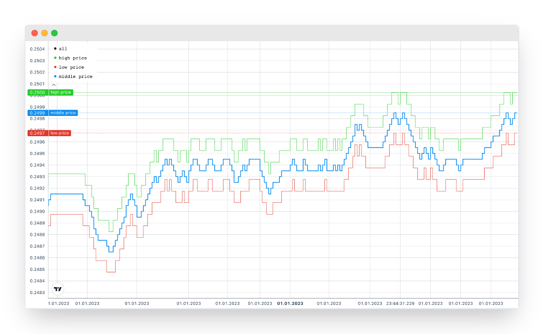
Here we calculate the average price between two time series of high and low prices.
```julia
using TimeArrays
julia> high_prices = ta_high_price_sample_data()
2416-element TimeArray{DateTime, Float64}:
TimeTick(2023-01-01T00:00:08.998, 0.2457)
TimeTick(2023-01-01T00:00:43.315, 0.2458)
⋮
TimeTick(2023-01-01T23:59:43.246, 0.25)
julia> low_prices = ta_low_price_sample_data()
2396-element TimeArray{DateTime, Float64}:
TimeTick(2023-01-01T00:00:08.995, 0.2456)
TimeTick(2023-01-01T00:00:43.319, 0.2457)
⋮
TimeTick(2023-01-01T23:59:43.252, 0.2499)
julia> (low_prices + high_prices) / 2
3930-element TimeArray{DateTime, Float64}:
TimeTick(2023-01-01T00:00:08.995, NaN)
TimeTick(2023-01-01T00:00:08.998, 0.24565)
⋮
TimeTick(2023-01-01T23:59:43.252, 0.24995)
```
Visualized with [LightweightCharts.jl](https://github.com/bhftbootcamp/LightweightCharts.jl).
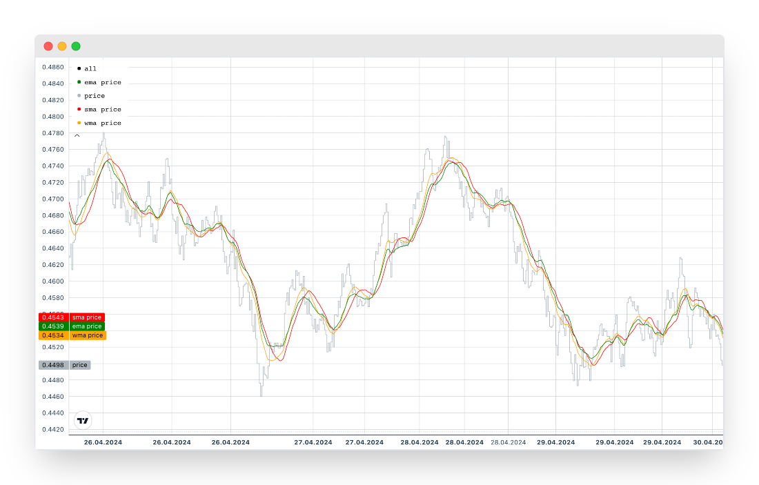
You can smooth the price data by using different [Moving Average](https://en.wikipedia.org/wiki/Moving_average) algorithms.
```julia
using TimeArrays
julia> prices = ta_price_sample_data()
7777-element TimeArray{DateTime, Float64}:
TimeTick(2024-04-01T00:00:00.661, 0.6501)
TimeTick(2024-04-01T00:05:57.481, 0.6505)
⋮
TimeTick(2024-04-30T23:42:11.920, 0.4417)
julia> sma_prices = ta_sma(prices, 20)
7777-element TimeArray{DateTime, Float64}:
TimeTick(2024-04-01T00:00:00.661, NaN)
TimeTick(2024-04-01T00:05:57.481, NaN)
⋮
TimeTick(2024-04-30T23:42:11.920, 0.4403)
julia> wma_prices = ta_wma(prices, 20)
7777-element TimeArray{DateTime, Float64}:
TimeTick(2024-04-01T00:00:00.661, NaN)
TimeTick(2024-04-01T00:05:57.481, NaN)
⋮
TimeTick(2024-04-30T23:42:11.920, 0.4409)
julia> ema_prices = ta_ema(prices, 20)
7777-element TimeArray{DateTime, Float64}:
TimeTick(2024-04-01T00:00:00.661, 0.6501)
TimeTick(2024-04-01T00:05:57.481, 0.6501)
⋮
TimeTick(2024-04-30T23:42:11.920, 0.4399)
```
Visualized with [LightweightCharts.jl](https://github.com/bhftbootcamp/LightweightCharts.jl).
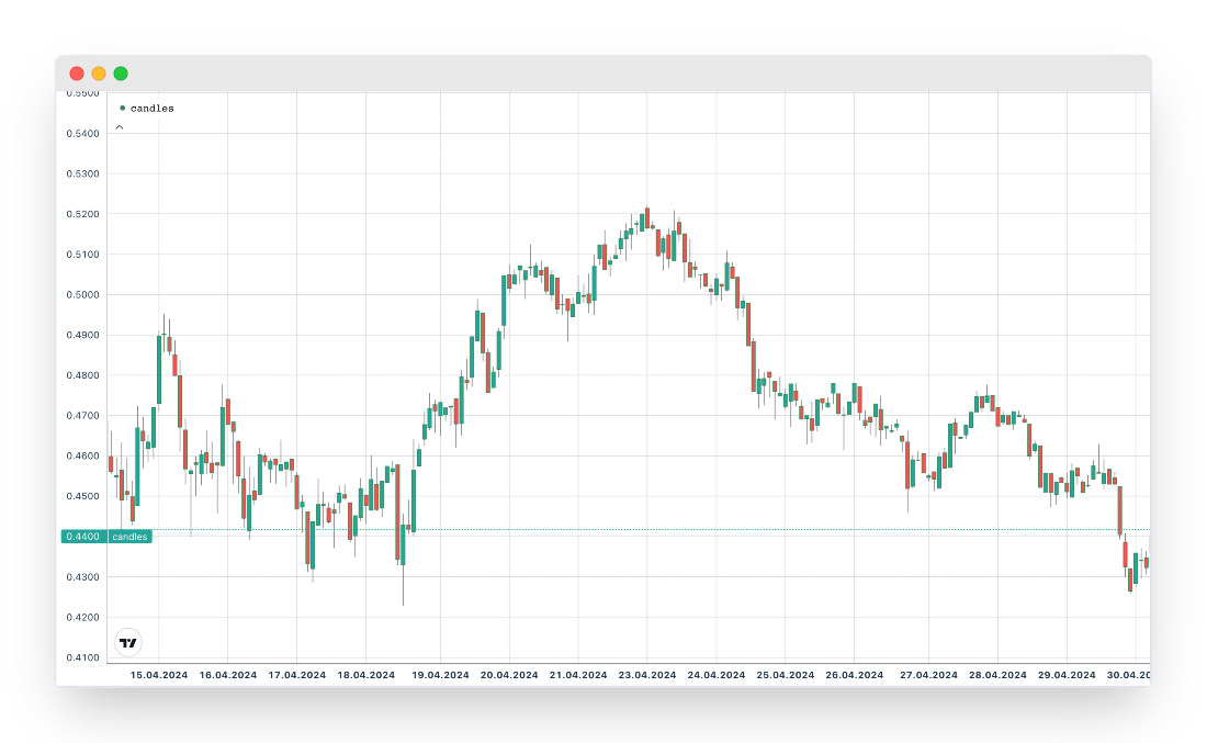
You can also use custom types with TimeArrays. Below we convert prices into four-hour candlesticks using resampling.
```julia
using Dates
using TimeArrays
struct OHLC
open::Float64
high::Float64
low::Float64
close::Float64
end
function ohlc(x::AbstractVector{<:Number})
return if isempty(x)
ta_nan(OHLC)
else
OHLC(x[1], maximum(x), minimum(x), x[end])
end
end
TimeArrays.ta_nan(::Type{OHLC}) = OHLC(NaN, NaN, NaN, NaN)
TimeArrays.return_type(::typeof(ohlc), ::Type{<:Number}) = OHLC
julia> prices = ta_price_sample_data()
7777-element TimeArray{DateTime, Float64}:
TimeTick(2024-04-01T00:00:00.661, 0.6501)
TimeTick(2024-04-01T00:05:57.481, 0.6505)
⋮
TimeTick(2024-04-30T23:42:11.920, 0.4417)
julia> ta_resample(ohlc, prices, Hour(2); closed = CLOSED_RIGHT, label = LABEL_RIGHT)
360-element TimeArray{DateTime, OHLC}:
TimeTick(2024-04-01T02:00:00, OHLC(0.6501, 0.6505, 0.6462, 0.6491))
TimeTick(2024-04-01T04:00:00, OHLC(0.6478, 0.6480, 0.6443, 0.6452))
⋮
TimeTick(2024-05-01T00:00:00, OHLC(0.4396, 0.4436, 0.4396, 0.4417))
```
Visualized with [LightweightCharts.jl](https://github.com/bhftbootcamp/LightweightCharts.jl).
## Tables.jl Integration
TimeArrays.jl provides seamless integration with the Tables.jl ecosystem, enabling easy interoperability with DataFrames, CSV files, and other tabular data formats.
```julia
using TimeArrays, DataFrames, CSV, Dates
import Tables
# Create a TimeArray
ta = TimeArray([DateTime("2024-01-01"), DateTime("2024-01-02")], [1.0, 2.0])
# Convert to DataFrame
df = DataFrame(ta)
# Convert to any Tables.jl-compatible format
table_data = Tables.columntable(ta)
# Create TimeArray from table data
ta_restored = TimeArray(table_data)
# Save to and load from CSV
CSV.write("data.csv", ta)
ta_from_csv = TimeArray(CSV.File("data.csv"))
```
For more details, see the [Tables.jl integration documentation](https://bhftbootcamp.github.io/TimeArrays.jl/stable/pages/tables/).
## Contributing
Contributions to TimeArrays are welcome! If you encounter a bug, have a feature request, or would like to contribute code, please open an issue or a pull request on GitHub.

 Visualized with [LightweightCharts.jl](https://github.com/bhftbootcamp/LightweightCharts.jl).
 Visualized with [LightweightCharts.jl](https://github.com/bhftbootcamp/LightweightCharts.jl).
 Visualized with [LightweightCharts.jl](https://github.com/bhftbootcamp/LightweightCharts.jl).