{
"cells": [
{
"cell_type": "markdown",
"metadata": {},
"source": [
"# Data Analysis with Jupyter Notebooks.\n",
"\n",
"# Tutorial 1 — Introducing Jupyter Notebooks\n",
"\n",
"Benjamin J. Morgan, University of Bath."
]
},
{
"cell_type": "markdown",
"metadata": {},
"source": [
"# Contents\n",
"\n",
"- [Data Analysis with Jupyter Notebooks](#intro)\n",
" - [Why analyse data with computer code?](#why)\n",
"- [Getting Started with Jupyter Notebooks](#getting_started)\n",
"- [Running Code](#running_code)\n",
"- [Saving Notebooks](#saving_notebooks)\n",
"- [Comments and Markdown cells](#comments)\n",
"- [Using assert Statements for Interactive Feedback](#assert_statements)"
]
},
{
"cell_type": "markdown",
"metadata": {},
"source": [
"# Data Analysis with Jupyter Notebooks\n",
"\n",
"This is a Jupyter notebook. In some ways each document is like a physical notebook. It can be used for describing an experiment, recording data, and commenting on it. Unlike a physical notebook, a Jupyter notebook also allows you to run and easily share computer code. This combination makes Jupyter notebooks a very useful tool for analysing data collected from experiments. Unlike spreadsheets or combinations of separate data analysis codes, a Jupyter notebook allows you to collect desciptions and notes for individual experiments, links to the raw data collected, the computer code that performs any necessary data analysis, and the final figures generated with these data, ready for use in a report or published paper.\n",
"\n",
"## Why analyse data using code?\n",
"Using computer code allows you to analyse experimental data *programmatically*. All the steps for working with your data are carried out according to a *program*; a predefined series of instructions; like a recipe for a particular meal. \n",
"\n",
"Once a particular program has been written, it will always produce the same results with the same starting data. This makes it possible to “show your working”. Scientists presenting new results can share their original data, alongside the code that they used for all their analysis. This has a number of benefits. Other scientists can review the code, run it against the original data set, and check that any analysis has been done correctly. \n",
"\n",
"Finished code can also be used as a starting point for looking at a similar set of data. The original scientist might repeat their experiment to confirm their results, or another group might collect data under slightly different conditions, and want to compare the two cases. Often the steps described by the code are the same for small data sets and for large data sets. Once an analysis program exists, processing enormous data sets simply becomes a question of access to sufficiently powerful computers. "
]
},
{
"cell_type": "markdown",
"metadata": {},
"source": [
"# Getting Started with Jupyter Notebooks\n",
"\n",
"A Jupyter notebook consists of a series of **cells** that contain text. These cells are arranged vertically, top-to-bottom in the document. Any cell can be edited by clicking on it. A cell in **edit mode** is indicated by a green border. \n",
" \n",
"A cell with a blue border is in **command mode**. \n",
"
\n",
"A cell with a blue border is in **command mode**. \n",
" \n",
"In command mode you are not able to type into a cell, but you can still edit the notebook (reordering cells, executing code, etc.) Commands for editing notebooks can be accessed from the manu at the top of the screen, and commonly used commands have keyboard shortcuts, which will be highlighted in the examples below. The full list of keyboard shortcuts can be found through **Help > Keyboard Shortcuts** in the menu, or by pressing **H**.\n",
"\n",
"To edit a cell in command mode, press enter or double click on the cell."
]
},
{
"cell_type": "markdown",
"metadata": {
"collapsed": true
},
"source": [
"## Running Code \n",
"\n",
"The Jupyter notebook is primarily useful for writing and running code. A large number of different computer languages can be used in Jupyter notebooks. In these examples, we will be using Python (specifically Python 3). Python is increasingly used across a large number of scientific disciplines for data management and analysis. The large scientific community means that very good resources already exist for data processing, such as the Jupyter project, and specific prewritten tools for manipulating and plotting data.\n",
"\n",
"This course will not go into detail about how to write your own Python code. Instead, as much as possible we are going to focus on learning how to use readily available packages for data analysis. There are plenty of resources for learning Python for more traditional programming tasks, such as the DataCamp [Learn Python for Data Science](https://www.datacamp.com/courses/intro-to-python-for-data-science) tutorial.\n",
"\n",
"The default cell type in a Jupyter notebook is a **code** cell. If you open a new notebook it will have one, empty, code cell. And you can always create more cells by clicking in the menu on **Insert > Insert Cell Above** (or press **A**) or **Insert > Insert Cell Below** (or press **B**). \n",
"
\n",
"In command mode you are not able to type into a cell, but you can still edit the notebook (reordering cells, executing code, etc.) Commands for editing notebooks can be accessed from the manu at the top of the screen, and commonly used commands have keyboard shortcuts, which will be highlighted in the examples below. The full list of keyboard shortcuts can be found through **Help > Keyboard Shortcuts** in the menu, or by pressing **H**.\n",
"\n",
"To edit a cell in command mode, press enter or double click on the cell."
]
},
{
"cell_type": "markdown",
"metadata": {
"collapsed": true
},
"source": [
"## Running Code \n",
"\n",
"The Jupyter notebook is primarily useful for writing and running code. A large number of different computer languages can be used in Jupyter notebooks. In these examples, we will be using Python (specifically Python 3). Python is increasingly used across a large number of scientific disciplines for data management and analysis. The large scientific community means that very good resources already exist for data processing, such as the Jupyter project, and specific prewritten tools for manipulating and plotting data.\n",
"\n",
"This course will not go into detail about how to write your own Python code. Instead, as much as possible we are going to focus on learning how to use readily available packages for data analysis. There are plenty of resources for learning Python for more traditional programming tasks, such as the DataCamp [Learn Python for Data Science](https://www.datacamp.com/courses/intro-to-python-for-data-science) tutorial.\n",
"\n",
"The default cell type in a Jupyter notebook is a **code** cell. If you open a new notebook it will have one, empty, code cell. And you can always create more cells by clicking in the menu on **Insert > Insert Cell Above** (or press **A**) or **Insert > Insert Cell Below** (or press **B**). \n",
" \n",
"Any code typed into a code cell can be run (or “**executed**”) by pressing `Shift-Enter` or pressing the
\n",
"Any code typed into a code cell can be run (or “**executed**”) by pressing `Shift-Enter` or pressing the  button in the notebook toolbar.\n",
"\n",
"This practical consists of an interactive tutorial (this notebook), followed by a a series of exercises. Some code cells in the tutorial will already have code in them, which you can **run** by selecting and pressing `Shift-Enter` or clicking the toolbar button:"
]
},
{
"cell_type": "code",
"execution_count": null,
"metadata": {},
"outputs": [],
"source": [
"2+3 # run this cell…"
]
},
{
"cell_type": "markdown",
"metadata": {},
"source": [
"You should now have Out[ ]: with the result of running this code printed next to it:\n",
"
button in the notebook toolbar.\n",
"\n",
"This practical consists of an interactive tutorial (this notebook), followed by a a series of exercises. Some code cells in the tutorial will already have code in them, which you can **run** by selecting and pressing `Shift-Enter` or clicking the toolbar button:"
]
},
{
"cell_type": "code",
"execution_count": null,
"metadata": {},
"outputs": [],
"source": [
"2+3 # run this cell…"
]
},
{
"cell_type": "markdown",
"metadata": {},
"source": [
"You should now have Out[ ]: with the result of running this code printed next to it:\n",
" \n",
"and the focus has automatically moved to the next cell. You can always re-select a cell to run it again.\n",
"\n",
"Most of the code examples will be presented like this:\n",
"\n",
">```python\n",
"print(\"hello\")\n",
"```\n",
"\n",
"with an empty code cell underneath. These examples are for you to type into the empty code cell and then run. Do not copy and paste these. You will learn the concepts faster and become comfortable with writing your own code if you type each piece of code out.\n",
"\n",
"Start with this example:\n",
"\n",
">```python\n",
"print(\"hello\")\n",
"```"
]
},
{
"cell_type": "code",
"execution_count": null,
"metadata": {},
"outputs": [],
"source": [
"print( \"hello\" )"
]
},
{
"cell_type": "markdown",
"metadata": {},
"source": [
"Your output should be\n",
"\n",
"```\n",
"hello\n",
"```"
]
},
{
"cell_type": "markdown",
"metadata": {},
"source": [
"There will also be small exercises that ask you to write your own piece of code from scratch, or modify an example that is not finished yet; it might contain an error – often called a **bug**, or just not do exactly what we would like. These will be indicated with green boxes."
]
},
{
"cell_type": "markdown",
"metadata": {},
"source": [
"
\n",
"and the focus has automatically moved to the next cell. You can always re-select a cell to run it again.\n",
"\n",
"Most of the code examples will be presented like this:\n",
"\n",
">```python\n",
"print(\"hello\")\n",
"```\n",
"\n",
"with an empty code cell underneath. These examples are for you to type into the empty code cell and then run. Do not copy and paste these. You will learn the concepts faster and become comfortable with writing your own code if you type each piece of code out.\n",
"\n",
"Start with this example:\n",
"\n",
">```python\n",
"print(\"hello\")\n",
"```"
]
},
{
"cell_type": "code",
"execution_count": null,
"metadata": {},
"outputs": [],
"source": [
"print( \"hello\" )"
]
},
{
"cell_type": "markdown",
"metadata": {},
"source": [
"Your output should be\n",
"\n",
"```\n",
"hello\n",
"```"
]
},
{
"cell_type": "markdown",
"metadata": {},
"source": [
"There will also be small exercises that ask you to write your own piece of code from scratch, or modify an example that is not finished yet; it might contain an error – often called a **bug**, or just not do exactly what we would like. These will be indicated with green boxes."
]
},
{
"cell_type": "markdown",
"metadata": {},
"source": [
" \n",
"Edit the print statement below, so that when you run the cell it prints your name.\n",
"
"
]
},
{
"cell_type": "markdown",
"metadata": {},
"source": [
"Missing code is indicated by a series of grey squares, which you will need to replace."
]
},
{
"cell_type": "code",
"execution_count": null,
"metadata": {},
"outputs": [],
"source": [
"# Edit this code cell and run it.\n",
"print(\"My name is ◽◽◽\")"
]
},
{
"cell_type": "markdown",
"metadata": {},
"source": [
"\n",
"Type new code into the cell below to print today's date.\n",
"
"
]
},
{
"cell_type": "code",
"execution_count": null,
"metadata": {},
"outputs": [],
"source": [
"# Edit this code cell and run it.\n",
"print( ◽◽◽ )"
]
},
{
"cell_type": "markdown",
"metadata": {},
"source": [
"## Saving Notebooks\n",
"\n",
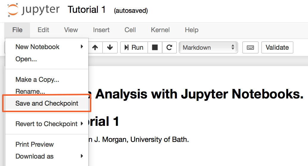
"To save your notebook, you can select **File > Save and Checkpoint** from the Jupyter menu, or use the keyboard shortcut **⌘+S** (on macOS) or **ctrl+S** (on Windows & Linux). Jupyter notebooks are saved as **.ipynb** files.\n",
"\n",
" \n",
"\n",
"You can make a copy of a notebook (for example, to save an old version while you work on a new idea, or to duplicate a notebook to a different directory) you can either select **File > Make a Copy**, which duplicates the current notebook in the same directory; or you can select **File > Download as > Notebook (.ipynb)**, to download a copy into your **Downloads**."
]
},
{
"cell_type": "markdown",
"metadata": {},
"source": [
"## Explain Your Code: Comments and Markdown Cells\n",
"One of the advantages of using *code* for numerical calculations and data analysis is that you end up with a record of exactly what you have done. You, or anyone else, can read the code, to understand how you reached your answer. You can think of this as “showing your working”, and it can be very helpful if you want to solve a *similar* problem in the future.\n",
"\n",
"Often, reading only the code can get quite cryptic (it is called “code”, after all), which makes it difficult to understand what is happening. To explain what a particular piece of code does, or to explain *why* a piece of code is being used, you can include **comments**.\n",
"\n",
" \n",
"```python\n",
"# this is a comment\n",
"```\n",
"\n",
"Any text that appears after a # symbol is part of the comment, and is ignored when the code is run. \n",
"\n",
"Jupyter notebooks offer a second way to describe what you are doing: **Markdown cells**. A code cell can be converted to a Markdown cell by selecting Cell > Cell Type > Markdown from the menu. \n",
"
\n",
"\n",
"You can make a copy of a notebook (for example, to save an old version while you work on a new idea, or to duplicate a notebook to a different directory) you can either select **File > Make a Copy**, which duplicates the current notebook in the same directory; or you can select **File > Download as > Notebook (.ipynb)**, to download a copy into your **Downloads**."
]
},
{
"cell_type": "markdown",
"metadata": {},
"source": [
"## Explain Your Code: Comments and Markdown Cells\n",
"One of the advantages of using *code* for numerical calculations and data analysis is that you end up with a record of exactly what you have done. You, or anyone else, can read the code, to understand how you reached your answer. You can think of this as “showing your working”, and it can be very helpful if you want to solve a *similar* problem in the future.\n",
"\n",
"Often, reading only the code can get quite cryptic (it is called “code”, after all), which makes it difficult to understand what is happening. To explain what a particular piece of code does, or to explain *why* a piece of code is being used, you can include **comments**.\n",
"\n",
" \n",
"```python\n",
"# this is a comment\n",
"```\n",
"\n",
"Any text that appears after a # symbol is part of the comment, and is ignored when the code is run. \n",
"\n",
"Jupyter notebooks offer a second way to describe what you are doing: **Markdown cells**. A code cell can be converted to a Markdown cell by selecting Cell > Cell Type > Markdown from the menu. \n",
" \n",
"A Markdown cell can be used to type plain text, which is displayed when the cell is run. Markdown cells are useful for documenting a notebook, particularly when you want to write something more detailed than a short comment. Markdown cells can also contain basic text formatting, links, images, and equations (more information is [here](http://jupyter-notebook.readthedocs.io/en/latest/examples/Notebook/Working%20With%20Markdown%20Cells.html))."
]
},
{
"cell_type": "markdown",
"metadata": {},
"source": [
"
\n",
"A Markdown cell can be used to type plain text, which is displayed when the cell is run. Markdown cells are useful for documenting a notebook, particularly when you want to write something more detailed than a short comment. Markdown cells can also contain basic text formatting, links, images, and equations (more information is [here](http://jupyter-notebook.readthedocs.io/en/latest/examples/Notebook/Working%20With%20Markdown%20Cells.html))."
]
},
{
"cell_type": "markdown",
"metadata": {},
"source": [
"\n",
"Type a comment into the cell below and run it.\n",
"
"
]
},
{
"cell_type": "code",
"execution_count": null,
"metadata": {},
"outputs": [],
"source": [
"◽◽◽"
]
},
{
"cell_type": "markdown",
"metadata": {},
"source": [
"\n",
"The cell below should be a Markdown cell, but it is currently a code cell. \n",
"First run the cell to see what happens.\n",
"Then change it into a **Markdown** cell, before re-running it. \n",
"
"
]
},
{
"cell_type": "code",
"execution_count": null,
"metadata": {},
"outputs": [],
"source": [
"Markdown cells allow you to type longer text to explain what your code is doing. \n",
"Setting this cell to Markdown, and running it will format the text for clearer reading. \n",
"Markdown also provides shorthand for including other features such as [links][cheatsheet].\n",
"\n",
"[cheatsheet]:https://github.com/adam-p/markdown-here/wiki/Markdown-Cheatsheet"
]
},
{
"cell_type": "markdown",
"metadata": {},
"source": [
"To edit a Markdown cell after it has been run, double-click on it to see the raw Markdown code."
]
},
{
"cell_type": "markdown",
"metadata": {},
"source": [
"\n",
"Double click on the Markdown output above that starts “*Markdown cells allow you to type longer text…*” and add the following Markdown code to it:
# My favourite meals are
\n",
"- Breakfast
\n",
"- Lunch
\n",
"- Brunch\n",
"
\n",
"
\n",
"\n",
"Then re-run the cell to view the formatted output."
]
},
{
"cell_type": "markdown",
"metadata": {},
"source": [
"## Using **assert** Statements for Interactive Feedback\n",
"\n",
"The exercise notebooks contain code cells with **assert** statements. These have been included so that you can test your code as you write it. \n",
"\n",
"An **assert** statement checks whether a particular condition is **true**, or **false**. If the specified condition is **false**, running the code will produce an AssertionError error. If this happens, go back to your code, and figure out the source of the error before moving on. If an **assert** statement runs without an error, your code works correctly and you can move on to the next part of the exercise.\n",
"\n",
"e.g. if this is given as a mini-exercise\n",
"\n",
" \n",
"Calculate two plus two.\n",
"
\n",
"\n",
"and you mistype the solution in the code cell below:"
]
},
{
"cell_type": "code",
"execution_count": null,
"metadata": {},
"outputs": [],
"source": [
"# enter your code in this cell\n",
"2+3"
]
},
{
"cell_type": "code",
"execution_count": null,
"metadata": {},
"outputs": [],
"source": [
"# this cell tests your code. You do not need to edit it.\n",
"assert _ == 4 \n",
"# the _ character refers to the output from the previous cell."
]
},
{
"cell_type": "markdown",
"metadata": {},
"source": [
"Because the calcualtion code gives the wrong result, the **assert** statement in the following cell fails, producing an AssertionError.\n",
"\n",
" \n",
"Correct the code above, and check that the test passes.\n",
"
"
]
}
],
"metadata": {
"kernelspec": {
"display_name": "Python [default]",
"language": "python",
"name": "python3"
},
"language_info": {
"codemirror_mode": {
"name": "ipython",
"version": 3
},
"file_extension": ".py",
"mimetype": "text/x-python",
"name": "python",
"nbconvert_exporter": "python",
"pygments_lexer": "ipython3",
"version": "3.6.2"
},
"latex_envs": {
"LaTeX_envs_menu_present": true,
"autoclose": false,
"autocomplete": true,
"bibliofile": "biblio.bib",
"cite_by": "apalike",
"current_citInitial": 1,
"eqLabelWithNumbers": true,
"eqNumInitial": 1,
"hotkeys": {
"equation": "Ctrl-E",
"itemize": "Ctrl-I"
},
"labels_anchors": false,
"latex_user_defs": false,
"report_style_numbering": false,
"user_envs_cfg": false
}
},
"nbformat": 4,
"nbformat_minor": 2
}