DataLab Cup 1: Predicting Appropriate Response
Fall 2017
%matplotlib inline
Competition Info
In this competition, you have to select the most appropriate response from 6 candidates based on previous chat message. You are provided with lines of total 8 tv programs as training data, and each program has serveral episodes. You also get a question collection which contains 1 chat history and 6 condidate responses for each question. Your goal is to learn a function that is able to predict the best response.
Dataset Format
Program01.csv~Program08.csvcontains total 8 tv program's linesQuestion.csvcontains total 500 questions, and each question includes chat and candidate options.
How to Submit Results?
You have to predict the correct response in Question.csv, and submit it to the Kaggle-In-Class online judge system. Following are some example actions:
| Action | Description |
|---|---|
| Data | Get the dataset. |
| Make a Submission | Your testing performance will be evaluated immediately and shown on the leaderboard. |
| Leaderboard | The current ranking of participants. Note that this ranking only reflects the performance on part of the testset and may not equal to the final ranking (see below). |
| Forum | You can ask questions or share findings here. |
| Kernels | You can create your jupyter notebook, run it, and keep it as private or public here. |
Scoring
The evaluation metric is CategorizationAccuracy. The ranking shown on the leaderboard before the end of competition reflects only the accuracy over part of Question.csv. However, this is not how we evaluate your final scores. After the competition, we combine accuracy over the entire Question.csv and your report as the final score.
There will be two baseline results, namely, Benchmark-60 and Benchmark-80. You have to outperform Benchmark-60 to get 60 points, and Benchmark-80 to get 80. Meanwhile, the higher accuracy you achieve, the higher the final score you will get.
Important Dates
- 2017/10/24 (TUE) - competition starts
- 2017/11/05 (SUN) 23:59pm - competition ends, final score announcement;
- 2017/11/07 (TUE) - winner team share;
- 2017/11/09 (THU) 23:59pm - report submission (iLMS);
Report
After the competition, each team have to hand in a report in Jupyter notebook format via the iLMS system. You report should include:
- Student ID, name of each team member
- How did you preprocess data (cleaning, feature engineering, etc.)?
- How did you build the classifier (model, training algorithm, special techniques, etc.)?
- Conclusions (interesting findings, pitfalls, takeaway lessons, etc.)?
The file name of your report must be DL_comp1_{Your Team number}_report.ipynb.
Hint 1: Feature Engineering is More Important Then You Expected
So far, we learn various machine learning techniques based on datasets where the date features are predefined. In many real-world applications, including this competition, we only get raw data and have to define the features ourself. Feature engineering is the process of using domain knowledge to create features that make machine learning algorithms work. While good modeling and training techniques help you make better predictions, feature engineering usually determines whether your task is "learnable".
import pandas as pd

NUM_PROGRAM = 8
programs = []
for i in range(1, NUM_PROGRAM+1):
    program = pd.read_csv('Program0%d.csv' % (i))

    print('Program %d' % (i))
    print('Episodes: %d' % (len(program)))
    print(program.columns)
    print(program.loc[:1]['Content'])
    print('')

    programs.append(program)
questions = pd.read_csv('Question.csv')

print('Question')
print('Episodes: %d' % (len(questions)))
print(questions.columns)
print(questions.loc[:2])
We get raw content of programs' lines, but there aren't any feature we can learn from. To predict from text, we have to go through several preprocessing steps first.
Preprocessing: Cut Words
Since chinese characters are continuous one by one, we have to cut them into meaningful words first. We use jieba with traditional chinese dictionary to cut our text. You can install jieba via pip.
pip install jiebaimport jieba
jieba.set_dictionary('big5_dict.txt')
example_str = '我討厭吃蘋果'
cut_example_str = jieba.lcut(example_str)
print(cut_example_str)
We cut not only Program.csv but also Question.csv, and save as list.
def jieba_lines(lines):
    cut_lines = []

    for line in lines:
        cut_line = jieba.lcut(line)
        cut_lines.append(cut_line)

    return cut_lines
cut_programs = []

for program in programs:
    n = len(program)
    cut_program = []

    for i in range(n):
        lines = program.loc[i]['Content'].split('\n')
        cut_program.append(jieba_lines(lines))

    cut_programs.append(cut_program)
print(len(cut_programs))
print(len(cut_programs[0]))
print(len(cut_programs[0][0]))
print(cut_programs[0][0][:3])
cut_questions = []
n = len(questions)

for i in range(n):
    cut_question = []
    lines = questions.loc[i]['Question'].split('\n')
    cut_question.append(jieba_lines(lines))

    for i in range(6):
        line = questions.loc[i]['Option%d' % (i)]
        cut_question.append(jieba.lcut(line))

    cut_questions.append(cut_question)
print(len(cut_questions))
print(len(cut_questions[0]))
print(cut_questions[0][0])

for i in range(1, 7):
    print(cut_questions[0][i])
import numpy as np

np.save('cut_Programs.npy', cut_programs)
np.save('cut_Questions.npy', cut_questions)
After saving, we can load them directly next time.
cut_programs = np.load('cut_Programs.npy')
cut_Question = np.load('cut_Questions.npy')
Preprocessing: Word Dictionary & Out-of-Vocabulary
There are many words after cutting, but not all of them is useful. The word too common or too rare can not give us information but may noise. We count the the number of occurrence for each word and remove useless one.
word_dict = dict()
def add_word_dict(w):
    if not w in word_dict:
        word_dict[w] = 1
    else:
        word_dict[w] += 1
for program in cut_programs:
    for lines in program:
        for line in lines:
            for w in line:
                add_word_dict(w)
for question in cut_questions:
    lines = question[0]
    for line in lines:
        for w in line:
            add_word_dict(w)

    for i in range(1, 7):
        line = question[i]
        for w in line:
            add_word_dict(w)
import operator

word_dict = sorted(word_dict.items(), key=operator.itemgetter(1), reverse=True)
VOC_SIZE = 15000
VOC_START = 20

voc_dict = word_dict[VOC_START:VOC_START+VOC_SIZE]
print(voc_dict[:10])
np.save('voc_dict.npy', voc_dict)
voc_dict = np.load('voc_dict.npy')
Now, voc_dict becomes better word dictionary, then we should replace those removed words aka out-of-vocabulary words into an unknown token in the following use.
Preprocessing: Generating Training Data
Though the format of question is to select one from six, our traing data only have continuous lines. Naively, i want to change the whole problem into a binary classification which means given two lines, my model want to judge these two are context or not.
import random

NUM_TRAIN = 10000
TRAIN_VALID_RATE = 0.7
def generate_training_data():
    Xs, Ys = [], []

    for i in range(NUM_TRAIN):
        pos_or_neg = random.randint(0, 1)

        if pos_or_neg==1:
            program_id = random.randint(0, NUM_PROGRAM-1)
            episode_id = random.randint(0, len(cut_programs[program_id])-1)
            line_id = random.randint(0, len(cut_programs[program_id][episode_id])-2)

            Xs.append([cut_programs[program_id][episode_id][line_id],
                       cut_programs[program_id][episode_id][line_id+1]])
            Ys.append(1)

        else:
            first_program_id = random.randint(0, NUM_PROGRAM-1)
            first_episode_id = random.randint(0, len(cut_programs[first_program_id])-1)
            first_line_id = random.randint(0, len(cut_programs[first_program_id][first_episode_id])-1)

            second_program_id = random.randint(0, NUM_PROGRAM-1)
            second_episode_id = random.randint(0, len(cut_programs[second_program_id])-1)
            second_line_id = random.randint(0, len(cut_programs[second_program_id][second_episode_id])-1)

            Xs.append([cut_programs[first_program_id][first_episode_id][first_line_id],
                       cut_programs[second_program_id][second_episode_id][second_line_id]])
            Ys.append(0)

    return Xs, Ys
Xs, Ys = generate_training_data()

x_train, y_train = Xs[:int(NUM_TRAIN*TRAIN_VALID_RATE)], Ys[:int(NUM_TRAIN*TRAIN_VALID_RATE)]
x_valid, y_valid = Xs[int(NUM_TRAIN*TRAIN_VALID_RATE):], Ys[int(NUM_TRAIN*TRAIN_VALID_RATE):]
Since machine learning models only accept numerical features, we must convert categorical features, such as tokens into a numerical form. In the next section, we introduce several commonly used models, including BoW, TF-IDF, and Feature Hashing that allows us to represent text as numerical feature vectors.
example_doc = []

for line in cut_programs[0][0]:
    example_line = ''
    for w in line:
        if w in voc_dict:
            example_line += w+' '

    example_doc.append(example_line)

print(example_doc[:10])
Word2Vec: BoW (Bag-Of-Words)
The idea behind bag-of-words model is to represent each document by occurrence of words, which can be summarized as the following steps:
- Build vocabulary dictionary by unique token from the entire set of documents;
- Represent each document by a vector, where each position corresponds to the occurrence of a vocabulary in dictionary.
Each vocabulary in BoW can be a single word (1-gram) or a sequence of n continuous words (n-gram). It has been shown empirically that 3-gram or 4-gram BoW models yield good performance in anti-spam email filtering application.
Here, we use Scikit-learn's implementation CountVectorizer to construct the BoW model:
import scipy as sp
from sklearn.feature_extraction.text import CountVectorizer

# ngram_range=(min, max), default: 1-gram => (1, 1)
count = CountVectorizer(ngram_range=(1, 1))

count.fit(example_doc)
BoW = count.vocabulary_
print('[vocabulary]\n')
for key in list(BoW.keys())[:10]:
    print('%s %d' % (key, BoW[key]))
The parameter ngram_range=(min-length, max-length) in CountVectorizer specifies the vocabulary to be {min-length}-gram to {max-length}-gram. For example ngram_range=(1, 2) will use both 1-gram and 2-gram as vocabularies. After constructing BoW model by calling fit(), you can access BoW vocabularies in its attribute vocubalary_, which is stored as Python dictionary that maps vocabulary to an integer index.
Let's transform the example documents into feature vectors:
# get matrix (doc_id, vocabulary_id) --> tf
doc_bag = count.transform(example_doc)
print('(did, vid)\ttf')
print(doc_bag[:10])

print('\nIs document-term matrix a scipy.sparse matrix? {}'.format(sp.sparse.issparse(doc_bag)))
Since each document contains only a small subset of vocabularies, CountVectorizer.transform() stores feature vectors as scipy.sparse matrix, where entry index is (document-index, vocabulary-index) pair, and the value is the term frequency---the number of times a vocabulary (term) occurs in a document.
Unfortunately, many Scikit-learn classifiers do not support input as sparse matrix now. We can convert doc_bag into a Numpy dense matrix:
doc_bag = doc_bag.toarray()
print(doc_bag[:10])

print('\nAfter calling .toarray(), is it a scipy.sparse matrix? {}'.format(sp.sparse.issparse(doc_bag)))
doc_bag = count.fit_transform(example_doc).toarray()

print("[most frequent vocabularies]")
bag_cnts = np.sum(doc_bag, axis=0)
top = 10
# [::-1] reverses a list since sort is in ascending order
for tok, v in zip(count.inverse_transform(np.ones(bag_cnts.shape[0]))[0][bag_cnts.argsort()[::-1][:top]],
                  np.sort(bag_cnts)[::-1][:top]):
    print('%s: %d' % (tok, v))
To find out most frequent words among documents, we first sum up vocabulary counts in documents, where axis=0 is the document index. Then, we sort the summed vocabulary count array in ascending order and get the sorted index by argsort(). Next, we revert the sorted list by [::-1], and feed into inverse_transform() to get corresponding vocabularies. Finally, we show the 10 most frequent vocabularies with their occurrence counts.
Next, we introduce the TF-IDF model that downweights frequently occurring words among the input documents.
Word2Vec: TF-IDF (Term-Frequency & Inverse-Document-Frequency)
TF-IDF model calculates not only the term-frequency (TF) as BoW model does, but also the document-frequency
(DF) of a term, which refers to the number of documents that contain this term. The TF-IDF score for a term is defined as
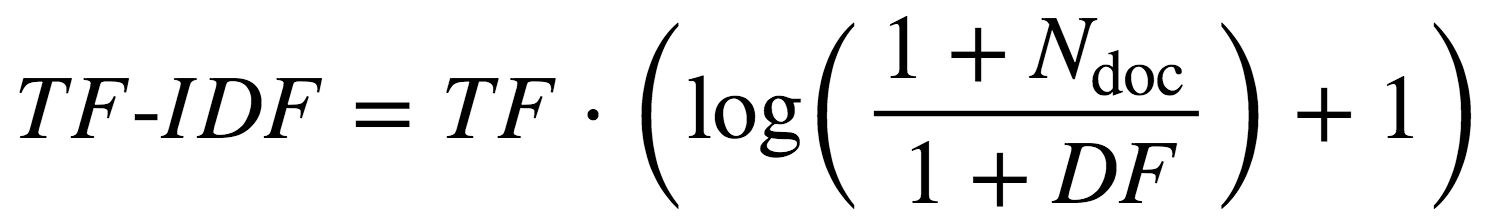
where the log() term is called the inverse-document-frequency (IDF) and Ndoc is the total number of documents. The idea behind TF-IDF is to downweight the TF of a word if it appears in many documents. For example, if a word appears in every document, the second term become log(1)+1=1 , which will be smaller than any other word appearing in only a part of documents.
NOTE: we add 1 to both the numerator and denominator inside the log() in the above definition so to avoid the numeric issue of dividing by 0.
Let's create the TF-IDF feature representation:
from sklearn.feature_extraction.text import TfidfVectorizer

tfidf = TfidfVectorizer(ngram_range=(1,1))
tfidf.fit(example_doc)

top = 10
# get idf score of vocabularies
idf = tfidf.idf_
print('[vocabularies with smallest idf scores]')
sorted_idx = idf.argsort()
for i in range(top):
    print('%s: %.2f' % (tfidf.get_feature_names()[sorted_idx[i]], idf[sorted_idx[i]]))

doc_tfidf = tfidf.transform(example_doc).toarray()
tfidf_sum = np.sum(doc_tfidf, axis=0)
print("\n[vocabularies with highest tf-idf scores]")
for tok, v in zip(tfidf.inverse_transform(np.ones(tfidf_sum.shape[0]))[0][tfidf_sum.argsort()[::-1]][:top],
                  np.sort(tfidf_sum)[::-1][:top]):
    print('%s: %f' % (tok, v))
Now we have a problem, the number of features that we have created in doc_tfidf is huge:
print(doc_tfidf.shape)
There are more than 500 features for merely 650 documents. In practice, this may lead to too much memory consumption (even with sparse matrix representation) if we have a large number of vocabularies.
Word2Vec: Feature Hashing
Feature hashing reduces the dimension vocabulary space by hashing each vocabulary into a hash table with a fixed number of buckets. As compared to BoW, feature hashing has the following pros and cons:
- (+) no need to store vocabulary dictionary in memory anymore
- (-) no way to map token index back to token via
inverse_transform() - (-) no IDF weighting
from sklearn.feature_extraction.text import HashingVectorizer

hashvec = HashingVectorizer(n_features=2**6)

doc_hash = hashvec.transform(example_doc)
print(doc_hash.shape)
Ok, now we can transform raw text to feature vectors.
More Creative Features
Now, you can go create your basic set of features for the text in competition. But don't stop from here. If you do aware the power of feature engineering, use your creativity to extract more features from the raw text. The more meaningful features you create, the more likely you will get a better score and win.
Here are few examples for inspiration:
- Word2Vec
- Doc2Vec
- TextRank
- Latent Dirichlet Allocation
- Similar word dictionary
- Part-of-speech Tagging
There are lots of other directions you can explore, such as NLP features, length of lines, etc.
Hint 2: Use Out-of-Core Learning If You Don't Have Enough Memory
The size of dataset in the competition is much larger than the lab. The dataset, after being represented as feature vectors, may become much larger, and you are unlikely to store all of them in memory. Next, we introduce another training technique called the Out of Core Learning to help you train a model using data streaming.
The idea of Out of Core Learning is similar to the stochastic gradient descent, which updates the model when seeing a minibatch, except that each minibatch is loaded from disk via a data stream. Since we only see a part of the dataset at a time, we can only use the HashingVectorizer to transform text into feature vectors because the HashingVectorizer does not require knowing the vocabulary space in advance.
Let's create a stream to read a chunk of CSV file at a time using the Pandas I/O API:
import pandas as pd

def get_stream(path, size):
    for chunk in pd.read_csv(path, chunksize=size):
        yield chunk

print(next(get_stream(path='imdb.csv', size=10)))
Good. Our stream works correctly.
For out-of core learning, we have to use models that can train and update the model's weight iteratively. Here, we use the SGDClassifier to train a LogisticRegressor using the stochastic gradient descent. We can partial update SGDClassifier by calling the partial_fit() method. Our workflow now becomes:
- Stream documents directly from disk to get a mini-batch (chunk) of documents;
- Preprocess: clean words in the mini-batch of documents;
- Word2vec: use HashingVectorizer to extract features from text;
- Update
SGDClassifierand go back to step 1.
import re
from bs4 import BeautifulSoup

def preprocessor(text):
    # remove HTML tags
    text = BeautifulSoup(text, 'html.parser').get_text()

    # regex for matching emoticons, keep emoticons, ex: :), :-P, :-D
    r = '(?::|;|=|X)(?:-)?(?:\)|\(|D|P)'
    emoticons = re.findall(r, text)
    text = re.sub(r, '', text)

    # convert to lowercase and append all emoticons behind (with space in between)
    # replace('-','') removes nose of emoticons
    text = re.sub('[\W]+', ' ', text.lower()) + ' ' + ' '.join(emoticons).replace('-','')
    return text

print(preprocessor('<a href="example.com">Hello, This :-( is a sanity check ;P!</a>'))
import nltk
from nltk.corpus import stopwords
from nltk.stem.porter import PorterStemmer

nltk.download('stopwords')
stop = stopwords.words('english')

def tokenizer_stem_nostop(text):
    porter = PorterStemmer()
    return [porter.stem(w) for w in re.split('\s+', text.strip()) \
            if w not in stop and re.match('[a-zA-Z]+', w)]

print(tokenizer_stem_nostop('runners like running and thus they run'))
from sklearn.feature_extraction.text import HashingVectorizer
from sklearn.linear_model import SGDClassifier
from sklearn.metrics import roc_auc_score

hashvec = HashingVectorizer(n_features=2**20,
                            preprocessor=preprocessor, tokenizer=tokenizer_stem_nostop)
# loss='log' gives logistic regression
clf = SGDClassifier(loss='log', n_iter=100)

batch_size = 1000
stream = get_stream(path='imdb.csv', size=batch_size)

classes = np.array([0, 1])
train_auc, val_auc = [], []

# we use one batch for training and another for validation in each iteration
iters = int((25000+batch_size-1)/(batch_size*2))

for i in range(iters):
    batch = next(stream)
    X_train, y_train = batch['review'], batch['sentiment']
    if X_train is None:
        break

    X_train = hashvec.transform(X_train)
    clf.partial_fit(X_train, y_train, classes=classes)
    train_auc.append(roc_auc_score(y_train, clf.predict_proba(X_train)[:,1]))

    # validate
    batch = next(stream)
    X_val, y_val = batch['review'], batch['sentiment']
    score = roc_auc_score(y_val, clf.predict_proba(hashvec.transform(X_val))[:,1])
    val_auc.append(score)
    print('[%d/%d] %f' % ((i+1)*(batch_size*2), 25000, score))
After fitting SGDClassifier by an entire pass over training set, let's plot the learning curve:
import matplotlib.pyplot as plt

plt.plot(range(1, len(train_auc)+1), train_auc, color='blue', label='Train auc')
plt.plot(range(1, len(train_auc)+1), val_auc, color='red', label='Val auc')
plt.legend(loc="best")
plt.xlabel('#Batches')
plt.ylabel('Auc')
plt.tight_layout()
plt.savefig('./fig-out-of-core.png', dpi=300)
plt.show()

The learning curve looks great! The validation accuracy improves as more examples are seen.
Since training SGDClassifier may take long, you can save your trained classifier to disk periodically:
# import optimized pickle written in C for serializing and  de-serializing a Python object
import _pickle as pkl

# dump to disk
pkl.dump(hashvec, open('hashvec.pkl', 'wb'))
pkl.dump(clf, open('clf-sgd.pkl', 'wb'))

# load from disk
hashvec = pkl.load(open('hashvec.pkl', 'rb'))
clf = pkl.load(open('clf-sgd.pkl', 'rb'))

df_test = pd.read_csv('imdb.csv')
print('test auc: %.3f' % roc_auc_score(df_test['sentiment'],
                                       clf.predict_proba(hashvec.transform(df_test['review']))[:,1]))
Now you have the all the supporting knowledge for the competition. Happy coding and good luck!