{
"cells": [
{
"cell_type": "markdown",
"metadata": {},
"source": [
"# Visualizing ASPECT unstructured mesh output with *yt*\n",
"\n",
"In this notebook, we present initial work towards visualizing standard output from the geodynamic code ASPECT in *yt*. \n",
"\n",
"We demonstrate two methods of loading data first using a simple dataset:"
]
},
{
"cell_type": "markdown",
"metadata": {},
"source": [
"1. [Manual Loading](#Manual-Loading)\n",
"2. [Loading with yt's new ASPECT frontend](#Loading-with-yt's-new-ASPECT-frontend)\n",
"\n",
"The first method uses the standard *yt* release, but requires manually loading mesh and field data from `.vtu` files into memory. The second method is more experimental and uses an early draft of a *yt*-native frontend for standard ASPECT output available on the `aspect` branch of the *yt* fork [here](https://github.com/chrishavlin/yt).\n",
"\n",
"After that, we show visualizations from a more complex simulation: [Visualizing fault formation in the lithosphere](#Visualizing-fault-formation-in-the-lithosphere)\n",
"\n",
"## Manual Loading\n",
"\n",
"In order to manually load data, we'll need the standard [*yt* release](https://yt-project.org/#getyt) along with [xmltodict](https://pypi.org/project/xmltodict/) and [meshio](https://pypi.org/project/meshio/). \n",
"\n",
"### pvtu data\n",
"\n",
"The standard ASPECT vtk output is comprised of unstructured mesh data stored in `.pvtu` files: each `.pvtu` file is a timestep from the ASPECT simulation and each `.pvtu` records the `.vtu` files storing the actual data (when running in parallel, each process will output a `.vtu` file). So in order to load this data into yt manually, we need to parse our `pvtu` files to assemble `connectivity`, `coordinates`and `node_data` arrays and supply them to `load_unstructured_mesh` function: \n",
"\n",
"```python\n",
"import yt \n",
"ds = yt.load_unstructured_mesh(\n",
" connectivity,\n",
" coordinates,\n",
" node_data = node_data\n",
")\n",
"```\n",
"\n",
"The following code creates a class to parse a `.pvtu` file and accompanying `.vtu` files using a combination of [xmltodict](https://pypi.org/project/xmltodict/) and [meshio](https://pypi.org/project/meshio/). After instantiating, `pvuFile.load()` will load each `.vtu` file into memory as a separate mesh to give to `load_unstructured_mesh`:"
]
},
{
"cell_type": "code",
"execution_count": 1,
"metadata": {},
"outputs": [],
"source": [
"import os \n",
"import numpy as np\n",
"import xmltodict, meshio\n",
"\n",
"class pvuFile(object):\n",
" def __init__(self,file,**kwargs):\n",
" self.file=file \n",
" self.dataDir=kwargs.get('dataDir',os.path.split(file)[0])\n",
" with open(file) as data:\n",
" self.pXML = xmltodict.parse(data.read())\n",
" \n",
" # store fields for convenience \n",
" self.fields=self.pXML['VTKFile']['PUnstructuredGrid']['PPointData']['PDataArray'] \n",
" \n",
" self.connectivity = None\n",
" self.coordinates = None\n",
" self.node_data = None\n",
" \n",
" def load(self): \n",
" \n",
" conlist=[] # list of 2D connectivity arrays \n",
" coordlist=[] # global, concatenated coordinate array \n",
" nodeDictList=[] # list of node_data dicts, same length as conlist \n",
"\n",
" con_offset=-1\n",
" pieces = self.pXML['VTKFile']['PUnstructuredGrid']['Piece']\n",
" if not isinstance(pieces,list):\n",
" pieces = [pieces]\n",
" \n",
" for mesh_id,src in enumerate(pieces):\n",
" print(f\"processing vtu file {mesh_id+1} of {len(pieces)}\")\n",
" mesh_name=\"connect{meshnum}\".format(meshnum=mesh_id+1) # connect1, connect2, etc. \n",
" \n",
" srcFi=os.path.join(self.dataDir,src['@Source']) # full path to .vtu file \n",
" \n",
" [con,coord,node_d]=self.loadPiece(srcFi,mesh_name,con_offset+1) \n",
" con_offset=con.max() \n",
" \n",
" conlist.append(con.astype(\"i8\"))\n",
" coordlist.extend(coord.astype(\"f8\"))\n",
" nodeDictList.append(node_d)\n",
" \n",
" self.connectivity=conlist\n",
" self.coordinates=np.array(coordlist)\n",
" self.node_data=nodeDictList\n",
" \n",
" def loadPiece(self,srcFi,mesh_name,connectivity_offset=0): \n",
" meshPiece=meshio.read(srcFi) # read it in with meshio \n",
" coords=meshPiece.points # coords and node_data are already global\n",
" cell_type = list(meshPiece.cells_dict.keys())[0]\n",
" \n",
" connectivity=meshPiece.cells_dict[cell_type] # 2D connectivity array \n",
"\n",
" # parse node data \n",
" node_data=self.parseNodeData(meshPiece.point_data,connectivity,mesh_name)\n",
"\n",
" # offset the connectivity matrix to global value \n",
" connectivity=np.array(connectivity)+connectivity_offset\n",
"\n",
" return [connectivity,coords,node_data]\n",
" \n",
" def parseNodeData(self,point_data,connectivity,mesh_name):\n",
" \n",
" # for each field, evaluate field data by index, reshape to match connectivity \n",
" con1d=connectivity.ravel() \n",
" conn_shp=connectivity.shape \n",
" \n",
" comp_hash={0:'cx',1:'cy',2:'cz'}\n",
" def rshpData(data1d):\n",
" return np.reshape(data1d[con1d],conn_shp)\n",
" \n",
" node_data={} \n",
" for fld in self.fields: \n",
" nm=fld['@Name']\n",
" if nm in point_data.keys():\n",
" if '@NumberOfComponents' in fld.keys() and int(fld['@NumberOfComponents'])>1:\n",
" # we have a vector, deal with components\n",
" for component in range(int(fld['@NumberOfComponents'])): \n",
" comp_name=nm+'_'+comp_hash[component] # e.g., velocity_cx \n",
" m_F=(mesh_name,comp_name) # e.g., ('connect1','velocity_cx')\n",
" node_data[m_F]=rshpData(point_data[nm][:,component])\n",
" else:\n",
" # just a scalar! \n",
" m_F=(mesh_name,nm) # e.g., ('connect1','T')\n",
" node_data[m_F]=rshpData(point_data[nm])\n",
" \n",
" return node_data"
]
},
{
"cell_type": "markdown",
"metadata": {},
"source": [
"Now lets set a `.pvtu` solution path then instantiate and load our `pvuFile`:"
]
},
{
"cell_type": "code",
"execution_count": 2,
"metadata": {},
"outputs": [
{
"name": "stdout",
"output_type": "stream",
"text": [
"processing vtu file 1 of 1\n"
]
}
],
"source": [
"DataDir=os.path.join(os.environ.get('ASPECTdatadir','./'),'output_yt_vtu','solution')\n",
"pFile=os.path.join(DataDir,'solution-00000.pvtu')\n",
"if os.path.isfile(pFile) is False:\n",
" print(\"data file not found\")\n",
" \n",
"pvuData=pvuFile(pFile)\n",
"pvuData.load() "
]
},
{
"cell_type": "markdown",
"metadata": {},
"source": [
"And now let's actually create a *yt* dataset:"
]
},
{
"cell_type": "code",
"execution_count": 3,
"metadata": {},
"outputs": [
{
"name": "stderr",
"output_type": "stream",
"text": [
"yt : [INFO ] 2020-11-25 15:05:06,275 Parameters: current_time = 0.0\n",
"yt : [INFO ] 2020-11-25 15:05:06,276 Parameters: domain_dimensions = [2 2 2]\n",
"yt : [INFO ] 2020-11-25 15:05:06,276 Parameters: domain_left_edge = [0. 0. 0.]\n",
"yt : [INFO ] 2020-11-25 15:05:06,276 Parameters: domain_right_edge = [110000. 110000. 110000.]\n",
"yt : [INFO ] 2020-11-25 15:05:06,277 Parameters: cosmological_simulation = 0.0\n"
]
}
],
"source": [
"import yt \n",
"ds = yt.load_unstructured_mesh(\n",
" pvuData.connectivity,\n",
" pvuData.coordinates,\n",
" node_data = pvuData.node_data,\n",
" length_unit = 'm'\n",
")"
]
},
{
"cell_type": "markdown",
"metadata": {},
"source": [
"Now that we have our data loaded as a *yt* dataset, we can do some fun things. First, let's check what fields we have:"
]
},
{
"cell_type": "code",
"execution_count": 4,
"metadata": {},
"outputs": [
{
"data": {
"text/plain": [
"[('all', 'T'),\n",
" ('all', 'crust_lower'),\n",
" ('all', 'crust_upper'),\n",
" ('all', 'current_cohesions'),\n",
" ('all', 'current_friction_angles'),\n",
" ('all', 'density'),\n",
" ('all', 'noninitial_plastic_strain'),\n",
" ('all', 'p'),\n",
" ('all', 'plastic_strain'),\n",
" ('all', 'plastic_yielding'),\n",
" ('all', 'strain_rate'),\n",
" ('all', 'velocity_cx'),\n",
" ('all', 'velocity_cy'),\n",
" ('all', 'velocity_cz'),\n",
" ('all', 'viscosity'),\n",
" ('connect1', 'T'),\n",
" ('connect1', 'crust_lower'),\n",
" ('connect1', 'crust_upper'),\n",
" ('connect1', 'current_cohesions'),\n",
" ('connect1', 'current_friction_angles'),\n",
" ('connect1', 'density'),\n",
" ('connect1', 'noninitial_plastic_strain'),\n",
" ('connect1', 'p'),\n",
" ('connect1', 'plastic_strain'),\n",
" ('connect1', 'plastic_yielding'),\n",
" ('connect1', 'strain_rate'),\n",
" ('connect1', 'velocity_cx'),\n",
" ('connect1', 'velocity_cy'),\n",
" ('connect1', 'velocity_cz'),\n",
" ('connect1', 'viscosity')]"
]
},
"execution_count": 4,
"metadata": {},
"output_type": "execute_result"
}
],
"source": [
"ds.field_list"
]
},
{
"cell_type": "markdown",
"metadata": {},
"source": [
"as an example of some simple functionality, we can find the min and max values of the whole domain by creating a YTRegion covering the whole domain and selecting the extrema:"
]
},
{
"cell_type": "code",
"execution_count": 5,
"metadata": {},
"outputs": [],
"source": [
"ad = ds.all_data()"
]
},
{
"cell_type": "code",
"execution_count": 6,
"metadata": {},
"outputs": [
{
"data": {
"text/plain": [
"unyt_array([ 273., 1613.], '(dimensionless)')"
]
},
"execution_count": 6,
"metadata": {},
"output_type": "execute_result"
}
],
"source": [
"ad.quantities.extrema(('all','T'))"
]
},
{
"cell_type": "markdown",
"metadata": {},
"source": [
"creating slice plots is similarlly easy: "
]
},
{
"cell_type": "code",
"execution_count": 7,
"metadata": {},
"outputs": [
{
"name": "stderr",
"output_type": "stream",
"text": [
"yt : [INFO ] 2020-11-25 15:05:13,952 xlim = 0.000000 110000.000000\n",
"yt : [INFO ] 2020-11-25 15:05:13,952 ylim = 0.000000 110000.000000\n",
"yt : [INFO ] 2020-11-25 15:05:13,953 xlim = 0.000000 110000.000000\n",
"yt : [INFO ] 2020-11-25 15:05:13,954 ylim = 0.000000 110000.000000\n",
"yt : [INFO ] 2020-11-25 15:05:13,954 Making a fixed resolution buffer of (('all', 'T')) 800 by 800\n"
]
},
{
"data": {
"text/html": [
" "
],
"text/plain": [
""
]
},
"execution_count": 7,
"metadata": {},
"output_type": "execute_result"
}
],
"source": [
"slc = yt.SlicePlot(ds,'x',('all','T'))\n",
"slc.set_cmap(('all','T'),'hot_r')\n",
"slc.set_log('T',False)"
]
},
{
"cell_type": "markdown",
"metadata": {},
"source": [
"## Loading with yt's new ASPECT frontend\n",
"\n",
"An initial draft frontend for ASPECT data is available on the `aspect` branch of the *yt* fork at: https://github.com/chrishavlin/yt. Until a PR is submitted and the `aspect` branch makes its way into the main yt repository, you can clone the fork, checkout the `aspect` branch and install from source with `pip install .` At present, you also have to manually install the meshio and xmltodict packages as for the section on [Manual Loading](#Manual-Loading). \n",
"\n",
"Once installed, we can load the data using the usual yt method:"
]
},
{
"cell_type": "code",
"execution_count": 8,
"metadata": {},
"outputs": [
{
"name": "stderr",
"output_type": "stream",
"text": [
"yt : [INFO ] 2020-11-25 15:05:29,458 Parameters: current_time = 0.0\n",
"yt : [INFO ] 2020-11-25 15:05:29,459 Parameters: domain_dimensions = [1 1 1]\n",
"yt : [INFO ] 2020-11-25 15:05:29,459 Parameters: domain_left_edge = [0. 0. 0.]\n",
"yt : [INFO ] 2020-11-25 15:05:29,459 Parameters: domain_right_edge = [100000. 100000. 100000.]\n",
"yt : [INFO ] 2020-11-25 15:05:29,460 Parameters: cosmological_simulation = 0\n",
"yt : [INFO ] 2020-11-25 15:05:29,486 detected cell type is hexahedron.\n"
]
}
],
"source": [
"import yt\n",
"ds = yt.load(pFile)"
]
},
{
"cell_type": "code",
"execution_count": 9,
"metadata": {},
"outputs": [
{
"name": "stderr",
"output_type": "stream",
"text": [
"yt : [INFO ] 2020-11-25 15:05:31,123 xlim = 0.000000 100000.000000\n",
"yt : [INFO ] 2020-11-25 15:05:31,124 ylim = 0.000000 100000.000000\n",
"yt : [INFO ] 2020-11-25 15:05:31,125 xlim = 0.000000 100000.000000\n",
"yt : [INFO ] 2020-11-25 15:05:31,125 ylim = 0.000000 100000.000000\n",
"yt : [INFO ] 2020-11-25 15:05:31,126 Making a fixed resolution buffer of (('all', 'T')) 800 by 800\n"
]
},
{
"data": {
"text/html": [
" "
],
"text/plain": [
""
]
},
"metadata": {},
"output_type": "display_data"
}
],
"source": [
"slc = yt.SlicePlot(ds,'x',('all','T'))\n",
"slc.set_cmap(('all','T'),'hot_r')\n",
"slc.show()"
]
},
{
"cell_type": "code",
"execution_count": 10,
"metadata": {},
"outputs": [
{
"name": "stderr",
"output_type": "stream",
"text": [
"yt : [INFO ] 2020-11-25 15:05:33,715 Saving plot figures/aspect_T_slice.png\n"
]
},
{
"data": {
"text/plain": [
"['figures/aspect_T_slice.png']"
]
},
"execution_count": 10,
"metadata": {},
"output_type": "execute_result"
}
],
"source": [
"slc.save('figures/aspect_T_slice.png')"
]
},
{
"cell_type": "code",
"execution_count": 11,
"metadata": {},
"outputs": [
{
"name": "stderr",
"output_type": "stream",
"text": [
"yt : [INFO ] 2020-11-25 15:05:34,597 xlim = 0.000000 100000.000000\n",
"yt : [INFO ] 2020-11-25 15:05:34,598 ylim = 0.000000 100000.000000\n",
"yt : [INFO ] 2020-11-25 15:05:34,599 xlim = 0.000000 100000.000000\n",
"yt : [INFO ] 2020-11-25 15:05:34,599 ylim = 0.000000 100000.000000\n",
"yt : [INFO ] 2020-11-25 15:05:34,600 Making a fixed resolution buffer of (('all', 'strain_rate')) 800 by 800\n"
]
},
{
"data": {
"text/html": [
" "
],
"text/plain": [
""
]
},
"metadata": {},
"output_type": "display_data"
}
],
"source": [
"slc = yt.SlicePlot(ds,'x',('all','strain_rate'))\n",
"slc.set_log('strain_rate',True)\n",
"slc.set_cmap(('all','strain_rate'),'kelp')\n",
"slc.show()"
]
},
{
"cell_type": "markdown",
"metadata": {},
"source": [
"As of now, the field data is not assigned units, so the color axes in these plots are unitless, but we can see we now have the expected units for the axes. \n"
]
},
{
"cell_type": "code",
"execution_count": 12,
"metadata": {},
"outputs": [
{
"name": "stderr",
"output_type": "stream",
"text": [
"yt : [INFO ] 2020-11-25 15:05:36,144 Saving plot figures/aspect_sr_slice.png\n"
]
},
{
"data": {
"text/plain": [
"['figures/aspect_sr_slice.png']"
]
},
"execution_count": 12,
"metadata": {},
"output_type": "execute_result"
}
],
"source": [
"slc.save('figures/aspect_sr_slice.png')"
]
},
{
"cell_type": "markdown",
"metadata": {},
"source": [
"## A note on higher order elements\n",
"\n",
"ASPECT can output higher order hexahedral elements but at present, *yt* only supports plotting first order elements. We could truncate the hexahedral elements to the first 8 nodes (the \"corner\" vertices for a linear element) before loading, but we can actually let *yt* do that automatically. Since we're using `meshio` on the back end for parsing the vtu files, however, we'll need a a modified version of meshio as the current vtu support does not include parsing the higher order elements. At present, installing the `vtu72` branch of the meshio fork at `https://github.com/chrishavlin/meshio` will allow *yt* to load the higher order data (though it will not be used in plotting). \n"
]
},
{
"cell_type": "markdown",
"metadata": {},
"source": [
"## Visualizing fault formation in the lithosphere\n",
"\n",
"The above examples are simple illustrations of loading and slicing ASPECT data with *yt*, but we can also load more complex ASPECT runs that were run in parallel. Here, we demsonstrate loading a complex simulation investigating fault formation in the lithosphere using the experimental yt-ASPECT loader noted above.\n",
"\n",
"This simulation models lithosphere extension with a pre-existing crustal weak zone. The weak zone is comprised of radomized variation in initial plastic strain, which together with a strain-softening brittle rheology leads to the ermergence of complex faulting networks that accomodate the stretching. \n",
"\n",
"So let's begin by loading up the dataset. This dataset is large -- all the datafiles for a single timestep end up at just over a GB of data, but we only need to load the mesh and connectivity arrays into memory along with the field that we're plotting. "
]
},
{
"cell_type": "code",
"execution_count": 15,
"metadata": {},
"outputs": [
{
"name": "stderr",
"output_type": "stream",
"text": [
"yt : [INFO ] 2020-11-25 15:06:26,808 Parameters: current_time = 0.0\n",
"yt : [INFO ] 2020-11-25 15:06:26,808 Parameters: domain_dimensions = [1 1 1]\n",
"yt : [INFO ] 2020-11-25 15:06:26,809 Parameters: domain_left_edge = [0. 0. 0.]\n",
"yt : [INFO ] 2020-11-25 15:06:26,809 Parameters: domain_right_edge = [500000. 500000. 100547.4453125]\n",
"yt : [INFO ] 2020-11-25 15:06:26,810 Parameters: cosmological_simulation = 0\n",
"yt : [INFO ] 2020-11-25 15:06:28,233 detected cell type is hexahedron.\n"
]
}
],
"source": [
"ds = yt.load('aspect/fault_formation/solution-00050.pvtu')"
]
},
{
"cell_type": "markdown",
"metadata": {},
"source": [
"In these simulations, faults show up most clearly in strain rate, so let's take some slices. Let's start with a vertical slice through the lithosphere:"
]
},
{
"cell_type": "code",
"execution_count": 16,
"metadata": {},
"outputs": [
{
"name": "stderr",
"output_type": "stream",
"text": [
"yt : [INFO ] 2020-11-25 15:07:20,097 xlim = 0.000000 500000.000000\n",
"yt : [INFO ] 2020-11-25 15:07:20,098 ylim = 0.000000 100547.445312\n",
"yt : [INFO ] 2020-11-25 15:07:20,098 xlim = 0.000000 500000.000000\n",
"yt : [INFO ] 2020-11-25 15:07:20,099 ylim = 0.000000 100547.445312\n",
"yt : [INFO ] 2020-11-25 15:07:20,099 Making a fixed resolution buffer of (('all', 'strain_rate')) 800 by 800\n"
]
},
{
"data": {
"text/html": [
" "
],
"text/plain": [
""
]
},
"metadata": {},
"output_type": "display_data"
}
],
"source": [
"slc = yt.SlicePlot(ds,'x',('all','strain_rate'))\n",
"slc.set_log('strain_rate',True)\n",
"slc.set_cmap(('all','strain_rate'),'magma')\n",
"slc.hide_axes()\n",
"slc.show()"
]
},
{
"cell_type": "markdown",
"metadata": {},
"source": [
"Now let's take a horizontal slice at fixed depth within the crust. To do this, we'll adjust provide a `center` argument to `SlicePlot` and set it to the domain center in `x` and `y` and set the `z` value to 90% of the maximum height: "
]
},
{
"cell_type": "code",
"execution_count": 17,
"metadata": {},
"outputs": [
{
"name": "stderr",
"output_type": "stream",
"text": [
"yt : [INFO ] 2020-11-25 15:07:54,728 xlim = 0.000000 500000.000000\n",
"yt : [INFO ] 2020-11-25 15:07:54,728 ylim = 0.000000 500000.000000\n",
"yt : [INFO ] 2020-11-25 15:07:54,729 xlim = 0.000000 500000.000000\n",
"yt : [INFO ] 2020-11-25 15:07:54,729 ylim = 0.000000 500000.000000\n",
"yt : [INFO ] 2020-11-25 15:07:54,730 Making a fixed resolution buffer of (('all', 'strain_rate')) 800 by 800\n"
]
},
{
"data": {
"text/html": [
" "
],
"text/plain": [
""
]
},
"metadata": {},
"output_type": "display_data"
}
],
"source": [
"c_val = ds.domain_center\n",
"c_arr = np.array([c_val[0],c_val[1],ds.domain_width[2]*0.9])\n",
"slc = yt.SlicePlot(ds,'z',('all','strain_rate'),center=c_arr)\n",
"slc.set_log('strain_rate',True)\n",
"slc.set_cmap(('all','strain_rate'),'magma')\n",
"slc.hide_axes()\n",
"slc.show()"
]
},
{
"cell_type": "markdown",
"metadata": {},
"source": [
"This map view shows the complex fault systems arising in this model of lithosphere extension. "
]
},
{
"cell_type": "markdown",
"metadata": {},
"source": [
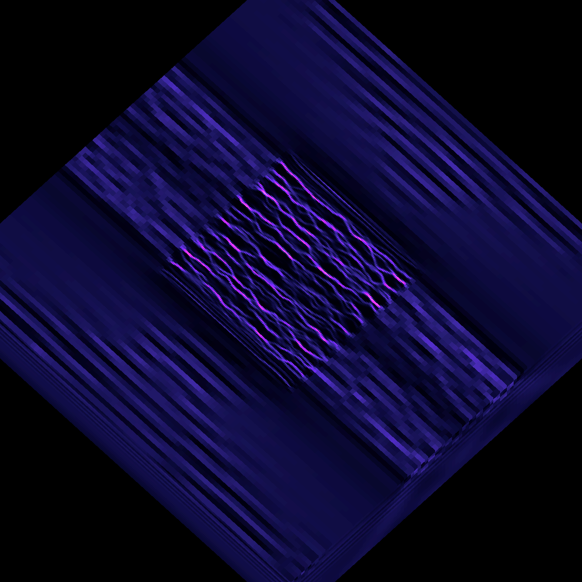
"### 3D rendering of aspect data\n",
"\n",
"In `aspect_mesh_source.py` in the `code/` folder, we demonstrate how to generate a 3D rendering of ASPECT data following the [Unstructured Mesh Rendering](https://yt-project.org/doc/visualizing/unstructured_mesh_rendering.html) documentation. In that script, we use some helper functions (in `code/mesh_animator`) to set a flight path that moves us around the volume and renders from different angles, including the following view:\n",
"\n",
""
]
},
{
"cell_type": "markdown",
"metadata": {},
"source": [
"The `aspect_mesh_source.py` script takes some time to run because it's rendering a large number of frames that can be [stitched together into an animation](https://i.imgur.com/QjYxff7.mp4). But the starting point to generate 3D renderings is just to create a 3D scene, adjust the view and then render the scene:\n",
"\n",
"```python\n",
"import yt \n",
"\n",
"ds = yt.load('aspect/fault_formation/solution-00050.pvtu')\n",
"sc = yt.create_scene(ds,('connect1','strain_rate')) # this is the slowest step \n",
"\n",
"```\n",
"We can then pull out the yt `MeshSource` object and modify the colormap:\n",
"\n",
"```python\n",
"ms = sc.get_source()\n",
"ms.cmap = 'magma'\n",
"ms.color_bounds = (1e-20,1e-14)\n",
"```\n",
"\n",
"And then adjust the camera settings:\n",
"\n",
"```python\n",
"cam = sc.camera\n",
"new_position = ds.arr([200.0, 200.0, 100.0], 'km')\n",
"north_vector = ds.arr([0.0, 0., 0.1], 'dimensionless')\n",
"cam.set_position(new_position, north_vector)\n",
"cam.set_width(ds.arr([300.0, 300.0, 300.0], 'km'))\n",
"```\n",
"To render and save the image, we can just call \n",
"\n",
"```\n",
"sc.save('image_file.png')\n",
"```\n",
"\n",
"**Check out [this link](https://i.imgur.com/QjYxff7.mp4) for the final animation constructed by combining the frames of the flight path generated by `code/aspect_mesh_source.py`.**\n"
]
},
{
"cell_type": "markdown",
"metadata": {},
"source": []
}
],
"metadata": {
"kernelspec": {
"display_name": "Python 3",
"language": "python",
"name": "python3"
},
"language_info": {
"codemirror_mode": {
"name": "ipython",
"version": 3
},
"file_extension": ".py",
"mimetype": "text/x-python",
"name": "python",
"nbconvert_exporter": "python",
"pygments_lexer": "ipython3",
"version": "3.7.8"
}
},
"nbformat": 4,
"nbformat_minor": 4
}