How to build a complicated, layered graphic
library(tidyverse)
library(knitr)
Charles Minard’s map of Napoleon’s disastrous Russian campaign of 1812

The graphic is notable for its representation in two dimensions of six types of data: the number of Napoleon’s troops; distance; temperature; the latitude and longitude; direction of travel; and location relative to specific dates.1
Building Minard’s map in R
# get data on troop movements and city names
troops <- read_table("data/minard-troops.txt")
## Parsed with column specification:
## cols(
## long = col_double(),
## lat = col_double(),
## survivors = col_integer(),
## direction = col_character(),
## group = col_integer()
## )cities <- read_table("data/minard-cities.txt")## Parsed with column specification:
## cols(
## long = col_double(),
## lat = col_double(),
## city = col_character()
## )troops## # A tibble: 51 x 5
## long lat survivors direction group
## <dbl> <dbl> <int> <chr> <int>
## 1 24.0 54.9 340000 A 1
## 2 24.5 55.0 340000 A 1
## 3 25.5 54.5 340000 A 1
## 4 26.0 54.7 320000 A 1
## 5 27.0 54.8 300000 A 1
## 6 28.0 54.9 280000 A 1
## 7 28.5 55.0 240000 A 1
## 8 29.0 55.1 210000 A 1
## 9 30.0 55.2 180000 A 1
## 10 30.3 55.3 175000 A 1
## # ... with 41 more rowscities## # A tibble: 20 x 3
## long lat city
## <dbl> <dbl> <chr>
## 1 24.0 55.0 Kowno
## 2 25.3 54.7 Wilna
## 3 26.4 54.4 Smorgoni
## 4 26.8 54.3 Moiodexno
## 5 27.7 55.2 Gloubokoe
## 6 27.6 53.9 Minsk
## 7 28.5 54.3 Studienska
## 8 28.7 55.5 Polotzk
## 9 29.2 54.4 Bobr
## 10 30.2 55.3 Witebsk
## 11 30.4 54.5 Orscha
## 12 30.4 53.9 Mohilow
## 13 32.0 54.8 Smolensk
## 14 33.2 54.9 Dorogobouge
## 15 34.3 55.2 Wixma
## 16 34.4 55.5 Chjat
## 17 36.0 55.5 Mojaisk
## 18 37.6 55.8 Moscou
## 19 36.6 55.3 Tarantino
## 20 36.5 55.0 Malo-JarosewiiExercise: Define the grammar of graphics for this graph
Click here for solution
- Layer
- Data -
troops - Mapping
- \(x\) and \(y\) - troop position (
latandlong) - Size -
survivors - Color -
direction
- \(x\) and \(y\) - troop position (
- Statistical transformation (stat) -
identity - Geometric object (geom) -
path - Position adjustment (position) - none
- Data -
- Layer
- Data -
cities - Mapping
- \(x\) and \(y\) - city position (
latandlong) - Label -
city
- \(x\) and \(y\) - city position (
- Statistical transformation (stat) -
identity - Geometric object (geom) -
text - Position adjustment (position) - none
- Data -
- Scale
- Size - range of widths for troop
path - Color - colors to indicate advancing or retreating troops
- Size - range of widths for troop
- Coordinate system - map projection (Mercator or something else)
- Faceting - none
Write the R code
First we want to build the layer for the troop movement:
plot_troops <- ggplot(data = troops, mapping = aes(x = long, y = lat)) +
  geom_path(aes(size = survivors,
                color = direction,
                group = group))
plot_troops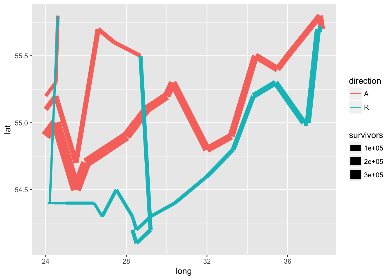
Next let’s add the cities layer:
plot_both <- plot_troops +
  geom_text(data = cities, mapping = aes(label = city), size = 4)
plot_both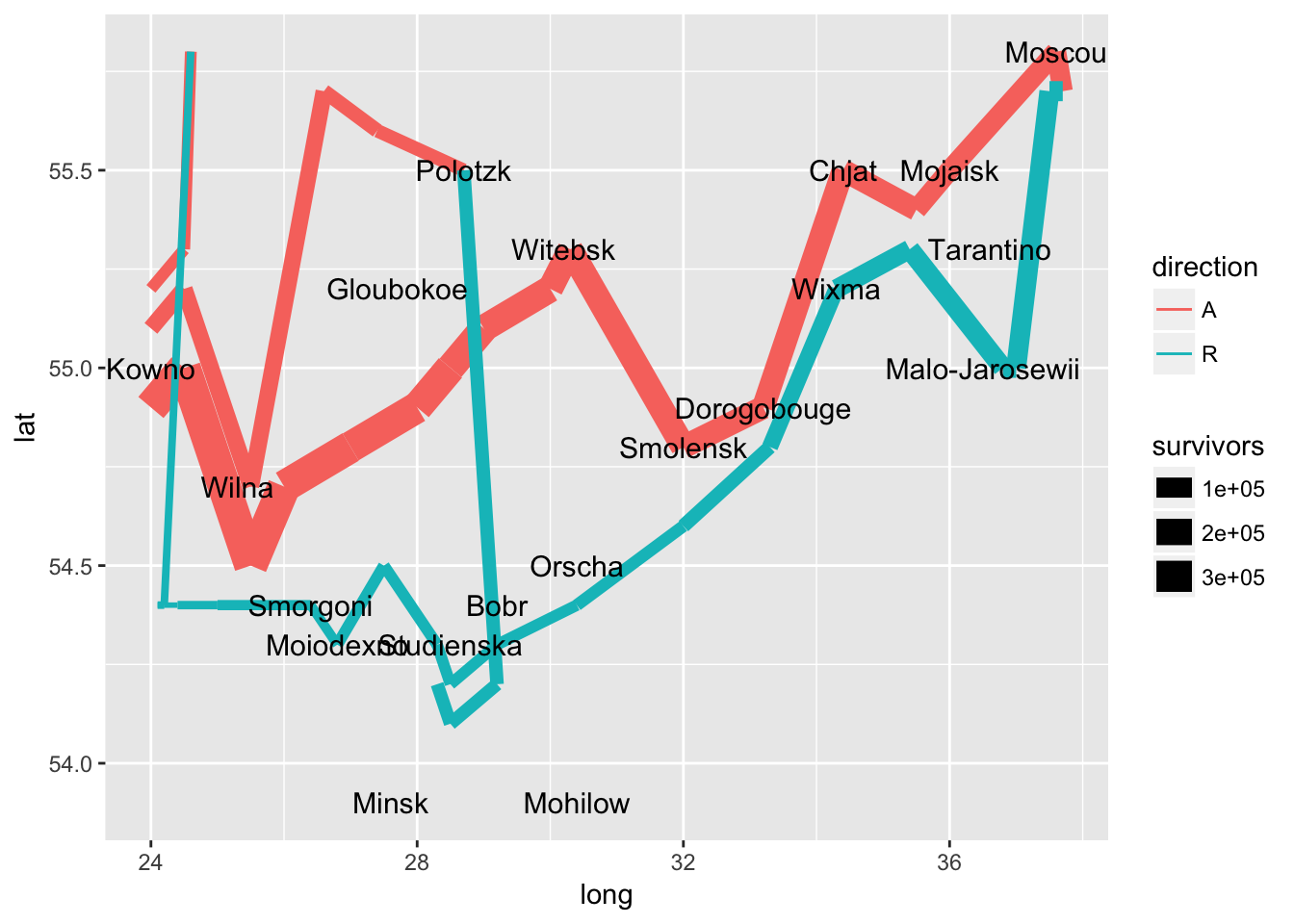
Now that the basic information is on there, we want to clean up the graph and polish the visualization by:
- Adjusting the size scale aesthetics for troop movement to better highlight the loss of troops over the campaign.
- Change the default colors to mimic Minard’s original grey and tan palette.
- Change the coordinate system to a map-based system that draws the \(x\) and \(y\) axes at equal intervals.
- Give the map a title and remove the axis labels.
plot_polished <- plot_both +
  scale_size(range = c(0, 12),
             breaks = c(10000, 20000, 30000),
             labels = c("10,000", "20,000", "30,000")) +
  scale_color_manual(values = c("tan", "grey50")) +
  coord_map() +
  labs(title = "Map of Napoleon's Russian campaign of 1812",
       x = NULL,
       y = NULL)
plot_polished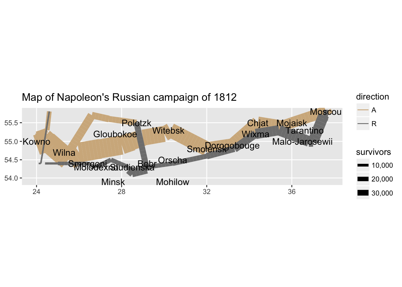
Finally we can change the default ggplot theme to remove the background and grid lines, as well as the legend:
plot_polished +
  theme_void() +
  theme(legend.position = "none")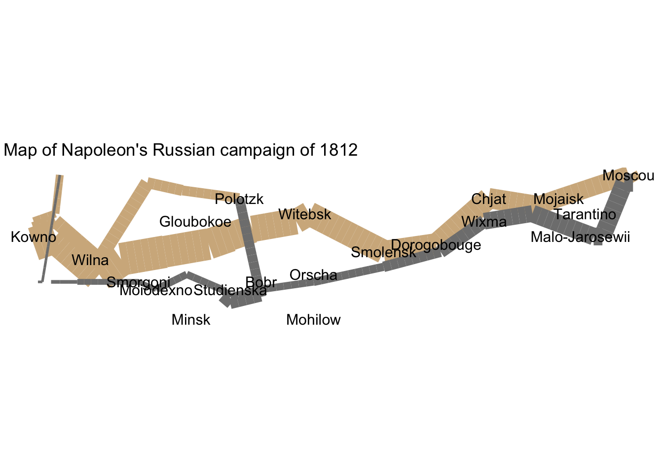
Session Info
devtools::session_info()## Session info -------------------------------------------------------------## setting value
## version R version 3.4.3 (2017-11-30)
## system x86_64, darwin15.6.0
## ui X11
## language (EN)
## collate en_US.UTF-8
## tz America/Chicago
## date 2018-03-12## Packages -----------------------------------------------------------------## package * version date source
## assertthat 0.2.0 2017-04-11 CRAN (R 3.4.0)
## backports 1.1.2 2017-12-13 CRAN (R 3.4.3)
## base * 3.4.3 2017-12-07 local
## bindr 0.1 2016-11-13 CRAN (R 3.4.0)
## bindrcpp 0.2 2017-06-17 CRAN (R 3.4.0)
## broom 0.4.3 2017-11-20 CRAN (R 3.4.1)
## cellranger 1.1.0 2016-07-27 CRAN (R 3.4.0)
## cli 1.0.0 2017-11-05 CRAN (R 3.4.2)
## colorspace 1.3-2 2016-12-14 CRAN (R 3.4.0)
## compiler 3.4.3 2017-12-07 local
## crayon 1.3.4 2017-10-03 Github (gaborcsardi/crayon@b5221ab)
## datasets * 3.4.3 2017-12-07 local
## devtools 1.13.5 2018-02-18 CRAN (R 3.4.3)
## digest 0.6.15 2018-01-28 CRAN (R 3.4.3)
## dplyr * 0.7.4.9000 2017-10-03 Github (tidyverse/dplyr@1a0730a)
## evaluate 0.10.1 2017-06-24 CRAN (R 3.4.1)
## forcats * 0.3.0 2018-02-19 CRAN (R 3.4.3)
## foreign 0.8-69 2017-06-22 CRAN (R 3.4.3)
## ggplot2 * 2.2.1 2016-12-30 CRAN (R 3.4.0)
## glue 1.2.0 2017-10-29 CRAN (R 3.4.2)
## graphics * 3.4.3 2017-12-07 local
## grDevices * 3.4.3 2017-12-07 local
## grid 3.4.3 2017-12-07 local
## gtable 0.2.0 2016-02-26 CRAN (R 3.4.0)
## haven 1.1.1 2018-01-18 CRAN (R 3.4.3)
## hms 0.4.1 2018-01-24 CRAN (R 3.4.3)
## htmltools 0.3.6 2017-04-28 CRAN (R 3.4.0)
## httr 1.3.1 2017-08-20 CRAN (R 3.4.1)
## jsonlite 1.5 2017-06-01 CRAN (R 3.4.0)
## knitr * 1.20 2018-02-20 CRAN (R 3.4.3)
## lattice 0.20-35 2017-03-25 CRAN (R 3.4.3)
## lazyeval 0.2.1 2017-10-29 CRAN (R 3.4.2)
## lubridate 1.7.2 2018-02-06 CRAN (R 3.4.3)
## magrittr 1.5 2014-11-22 CRAN (R 3.4.0)
## memoise 1.1.0 2017-04-21 CRAN (R 3.4.0)
## methods * 3.4.3 2017-12-07 local
## mnormt 1.5-5 2016-10-15 CRAN (R 3.4.0)
## modelr 0.1.1 2017-08-10 local
## munsell 0.4.3 2016-02-13 CRAN (R 3.4.0)
## nlme 3.1-131.1 2018-02-16 CRAN (R 3.4.3)
## parallel 3.4.3 2017-12-07 local
## pillar 1.1.0 2018-01-14 CRAN (R 3.4.3)
## pkgconfig 2.0.1 2017-03-21 CRAN (R 3.4.0)
## plyr 1.8.4 2016-06-08 CRAN (R 3.4.0)
## psych 1.7.8 2017-09-09 CRAN (R 3.4.1)
## purrr * 0.2.4 2017-10-18 CRAN (R 3.4.2)
## R6 2.2.2 2017-06-17 CRAN (R 3.4.0)
## Rcpp 0.12.15 2018-01-20 CRAN (R 3.4.3)
## readr * 1.1.1 2017-05-16 CRAN (R 3.4.0)
## readxl 1.0.0 2017-04-18 CRAN (R 3.4.0)
## reshape2 1.4.3 2017-12-11 CRAN (R 3.4.3)
## rlang 0.2.0 2018-02-20 cran (@0.2.0)
## rmarkdown 1.8 2017-11-17 CRAN (R 3.4.2)
## rprojroot 1.3-2 2018-01-03 CRAN (R 3.4.3)
## rstudioapi 0.7 2017-09-07 CRAN (R 3.4.1)
## rvest 0.3.2 2016-06-17 CRAN (R 3.4.0)
## scales 0.5.0 2017-08-24 cran (@0.5.0)
## stats * 3.4.3 2017-12-07 local
## stringi 1.1.6 2017-11-17 CRAN (R 3.4.2)
## stringr * 1.3.0 2018-02-19 CRAN (R 3.4.3)
## tibble * 1.4.2 2018-01-22 CRAN (R 3.4.3)
## tidyr * 0.8.0 2018-01-29 CRAN (R 3.4.3)
## tidyverse * 1.2.1 2017-11-14 CRAN (R 3.4.2)
## tools 3.4.3 2017-12-07 local
## utils * 3.4.3 2017-12-07 local
## withr 2.1.1 2017-12-19 CRAN (R 3.4.3)
## xml2 1.2.0 2018-01-24 CRAN (R 3.4.3)
## yaml 2.1.16 2017-12-12 CRAN (R 3.4.3)This work is licensed under the CC BY-NC 4.0 Creative Commons License.