The first step is to calculate the age of each plane. To do that, use planes and the age variable:

plane_ages <- planes %>%
  mutate(age = 2013 - year) %>%
  select(tailnum, age)

The best approach to answering this question is a visualization. There are several different types of visualizations you could implement (e.g. scatterplot with smoothing line, line graph of average delay by age). The important thing is that we need to combine flights with plane_ages to determine for each flight the age of the plane. This is another mutating join. The best choice is inner_join() as this will automatically remove any rows in flights where we don’t have age data on the plane.

# smoothing line
flights %>%
  inner_join(plane_ages) %>%
  ggplot(aes(age, dep_delay)) +
  geom_smooth()

## Joining, by = "tailnum"

## `geom_smooth()` using method = 'gam'

## Warning: Removed 9374 rows containing non-finite values (stat_smooth).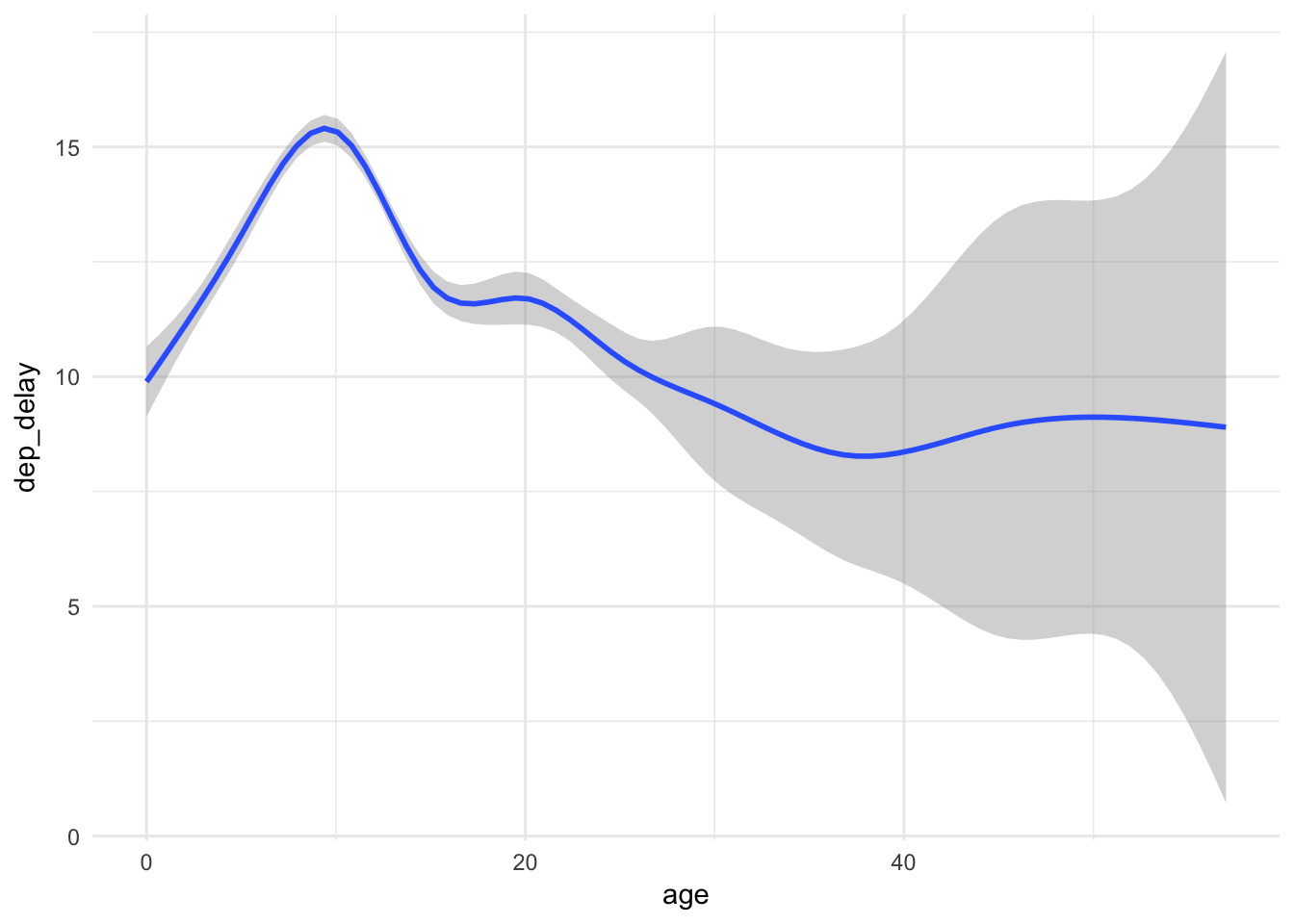

# line graph of average delay by age
flights %>%
  inner_join(plane_ages) %>%
  group_by(age) %>%
  summarise(delay = mean(dep_delay, na.rm = TRUE)) %>%
  ggplot(aes(age, delay)) +
  geom_point() +
  geom_line()

## Joining, by = "tailnum"

## Warning: Removed 1 rows containing missing values (geom_point).

## Warning: Removed 1 rows containing missing values (geom_path).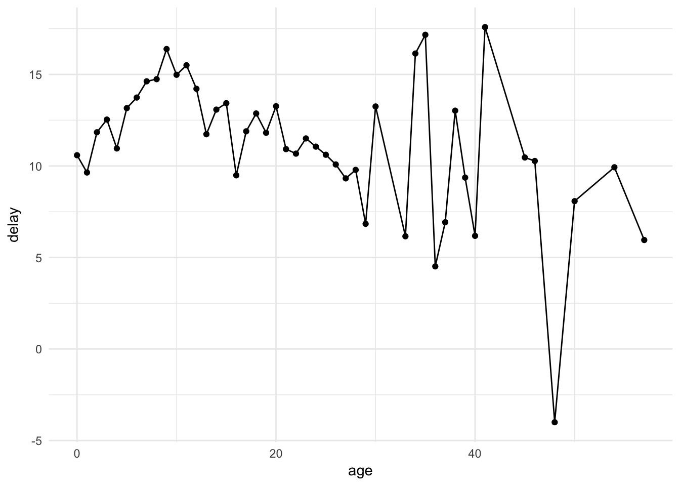

In this situation, left_join() could also be used because ggplot() and mean(na.rm = TRUE) drop missing values (remember that left_join() keeps all rows from flights, even if we don’t have information on the plane).

flights %>%
  left_join(plane_ages) %>%
  ggplot(aes(age, dep_delay)) +
  geom_smooth()

## Joining, by = "tailnum"

## `geom_smooth()` using method = 'gam'

## Warning: Removed 61980 rows containing non-finite values (stat_smooth).

flights %>%
  left_join(plane_ages) %>%
  group_by(age) %>%
  summarise(delay = mean(dep_delay, na.rm = TRUE)) %>%
  ggplot(aes(age, delay)) +
  geom_point() +
  geom_line()

## Joining, by = "tailnum"

## Warning: Removed 2 rows containing missing values (geom_point).

## Warning: Removed 2 rows containing missing values (geom_path).

The important takeaway is that departure delays do not appear to increase with plane age – in fact they seem to decrease slightly (though with an expanding confidence interval). Care to think of a reason why this may be so?

This is a mutating join, and the basic function you need to use here is left_join(). We have to perform the joining operation twice since we want to create new variables based on both the destination airport and the origin airport. And because the name of the key variable differs between the data frames, we need to explicitly define how to join the data frames using the by argument:

flights %>%
  left_join(airports, by = c(dest = "faa")) %>%
  left_join(airports, by = c(origin = "faa"))

## # A tibble: 336,776 x 33
##     year month   day dep_time sched_dep_time dep_delay arr_time
##    <int> <int> <int>    <int>          <int>     <dbl>    <int>
##  1  2013     1     1      517            515         2      830
##  2  2013     1     1      533            529         4      850
##  3  2013     1     1      542            540         2      923
##  4  2013     1     1      544            545        -1     1004
##  5  2013     1     1      554            600        -6      812
##  6  2013     1     1      554            558        -4      740
##  7  2013     1     1      555            600        -5      913
##  8  2013     1     1      557            600        -3      709
##  9  2013     1     1      557            600        -3      838
## 10  2013     1     1      558            600        -2      753
## # ... with 336,766 more rows, and 26 more variables: sched_arr_time <int>,
## #   arr_delay <dbl>, carrier <chr>, flight <int>, tailnum <chr>,
## #   origin <chr>, dest <chr>, air_time <dbl>, distance <dbl>, hour <dbl>,
## #   minute <dbl>, time_hour <dttm>, name.x <chr>, lat.x <dbl>,
## #   lon.x <dbl>, alt.x <int>, tz.x <dbl>, dst.x <chr>, tzone.x <chr>,
## #   name.y <chr>, lat.y <dbl>, lon.y <dbl>, alt.y <int>, tz.y <dbl>,
## #   dst.y <chr>, tzone.y <chr>

Notice that with this approach, we are joining all of the columns in airports. The instructions just asked for latitude and longitude, so we can create a copy of airports that only includes the necessary variables (lat and lon, plus the primary key variable faa) and join flights to that data frame:

airports_lite <- airports %>%
  select(faa, lat, lon)

flights %>%
  left_join(airports_lite, by = c(dest = "faa")) %>%
  left_join(airports_lite, by = c(origin = "faa"))

## # A tibble: 336,776 x 23
##     year month   day dep_time sched_dep_time dep_delay arr_time
##    <int> <int> <int>    <int>          <int>     <dbl>    <int>
##  1  2013     1     1      517            515         2      830
##  2  2013     1     1      533            529         4      850
##  3  2013     1     1      542            540         2      923
##  4  2013     1     1      544            545        -1     1004
##  5  2013     1     1      554            600        -6      812
##  6  2013     1     1      554            558        -4      740
##  7  2013     1     1      555            600        -5      913
##  8  2013     1     1      557            600        -3      709
##  9  2013     1     1      557            600        -3      838
## 10  2013     1     1      558            600        -2      753
## # ... with 336,766 more rows, and 16 more variables: sched_arr_time <int>,
## #   arr_delay <dbl>, carrier <chr>, flight <int>, tailnum <chr>,
## #   origin <chr>, dest <chr>, air_time <dbl>, distance <dbl>, hour <dbl>,
## #   minute <dbl>, time_hour <dttm>, lat.x <dbl>, lon.x <dbl>, lat.y <dbl>,
## #   lon.y <dbl>

This is better, but now we have two sets of latitude and longitude variables in the data frame: one for the destination airport, and one for the origin airport. When we perform the second left_join() operation, to avoid duplicate variable names the function automatically adds generic .x and .y suffixes to the output to disambiguate them. This is nice, but we might want something more intuitive to explicitly identify which variables are associated with the destination vs. the origin. To do that, we override the default suffix argument with custom suffixes:

airports_lite <- airports %>%
  select(faa, lat, lon)

flights %>%
  left_join(airports_lite, by = c(dest = "faa")) %>%
  left_join(airports_lite, by = c(origin = "faa"), suffix = c(".dest", ".origin"))

## # A tibble: 336,776 x 23
##     year month   day dep_time sched_dep_time dep_delay arr_time
##    <int> <int> <int>    <int>          <int>     <dbl>    <int>
##  1  2013     1     1      517            515         2      830
##  2  2013     1     1      533            529         4      850
##  3  2013     1     1      542            540         2      923
##  4  2013     1     1      544            545        -1     1004
##  5  2013     1     1      554            600        -6      812
##  6  2013     1     1      554            558        -4      740
##  7  2013     1     1      555            600        -5      913
##  8  2013     1     1      557            600        -3      709
##  9  2013     1     1      557            600        -3      838
## 10  2013     1     1      558            600        -2      753
## # ... with 336,766 more rows, and 16 more variables: sched_arr_time <int>,
## #   arr_delay <dbl>, carrier <chr>, flight <int>, tailnum <chr>,
## #   origin <chr>, dest <chr>, air_time <dbl>, distance <dbl>, hour <dbl>,
## #   minute <dbl>, time_hour <dttm>, lat.dest <dbl>, lon.dest <dbl>,
## #   lat.origin <dbl>, lon.origin <dbl>