Tidy data
library(tidyverse)Most data analysts and statisticians analyze data in a spreadsheet or tabular format. This is not the only way to store information,1 however in the social sciences it has been the paradigm for many decades. Tidy data is a specific way of organizing data into a consistent format which plugs into the tidyverse set of packages for R. It is not the only way to store data and there are reasons why you might not store data in this format, but eventually you will probably need to convert your data to a tidy format in order to efficiently analyze it.
There are three rules which make a dataset tidy:
- Each variable must have its own column.
- Each observation must have its own row.
- Each value must have its own cell.
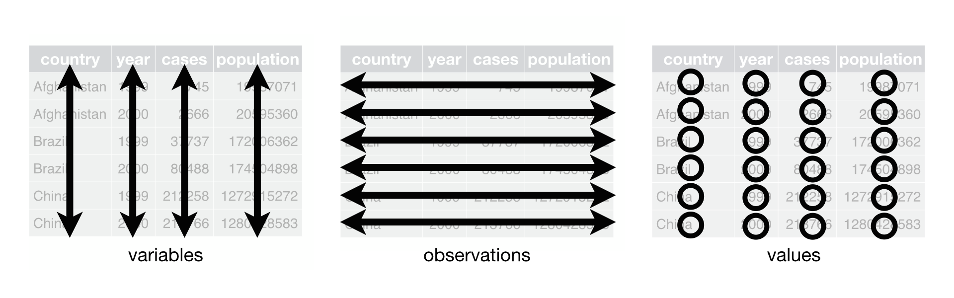
Figure 12.1 from R for Data Science
Let’s review the different tasks for tidying data using the R for Data Science gapminder subset. This is the data in a tidy format:
table1## # A tibble: 6 x 4
## country year cases population
## <chr> <int> <int> <int>
## 1 Afghanistan 1999 745 19987071
## 2 Afghanistan 2000 2666 20595360
## 3 Brazil 1999 37737 172006362
## 4 Brazil 2000 80488 174504898
## 5 China 1999 212258 1272915272
## 6 China 2000 213766 1280428583Note that in this data frame, each variable is in its own column (country, year, cases, and population), each observation is in its own row (i.e. each row is a different country-year pairing), and each value has its own cell.
Gathering
Gathering entails bringing a variable spread across multiple columns into a single column. For example, this version of table1 is not tidy because the year variable is spread across multiple columns:
table4a## # A tibble: 3 x 3
## country `1999` `2000`
## * <chr> <int> <int>
## 1 Afghanistan 745 2666
## 2 Brazil 37737 80488
## 3 China 212258 213766We can use the gather() function from the tidyr package to reshape the data frame and make this tidy. To do this we need three pieces of information:
- The names of the columns that represent the values, not variables. Here, those are
1999and2000. - The
key, or the name of the variable whose values form the column names. Here that isyear. - The
value, or the name of the variable whose values are spread over the cells. Here that iscases.
Notice that we create the names for
keyandvalue- they do not already exist in the data frame.
We implement this using the gather() function:
table4a %>%
  gather(`1999`, `2000`, key = "year", value = "cases")
## # A tibble: 6 x 3
## country year cases
## <chr> <chr> <int>
## 1 Afghanistan 1999 745
## 2 Brazil 1999 37737
## 3 China 1999 212258
## 4 Afghanistan 2000 2666
## 5 Brazil 2000 80488
## 6 China 2000 213766In Stata and other statistics software, this operation would be called reshaping data wide to long.
Spreading
Spreading brings an observation spread across multiple rows into a single row. It is the reverse of gathering. For instance, take table2:
table2## # A tibble: 12 x 4
## country year type count
## <chr> <int> <chr> <int>
## 1 Afghanistan 1999 cases 745
## 2 Afghanistan 1999 population 19987071
## 3 Afghanistan 2000 cases 2666
## 4 Afghanistan 2000 population 20595360
## 5 Brazil 1999 cases 37737
## 6 Brazil 1999 population 172006362
## 7 Brazil 2000 cases 80488
## 8 Brazil 2000 population 174504898
## 9 China 1999 cases 212258
## 10 China 1999 population 1272915272
## 11 China 2000 cases 213766
## 12 China 2000 population 1280428583It violates the tidy data principle because each observation (unit of analysis is a country-year pairing) is split across multiple rows. To tidy the data frame, we need to know:
- The
keycolumn, or the column that contains variable names. Here, it istype. - The
valuecolumn, or the column that contains values for multiple variables. Here it iscount.
Notice that unlike for gathering, when spreading the
keyandvaluecolumns are already defined in the data frame. We do not create the names ourselves, only identify them in the existing data frame.
table2 %>%
  spread(key = type, value = count)
## # A tibble: 6 x 4
## country year cases population
## * <chr> <int> <int> <int>
## 1 Afghanistan 1999 745 19987071
## 2 Afghanistan 2000 2666 20595360
## 3 Brazil 1999 37737 172006362
## 4 Brazil 2000 80488 174504898
## 5 China 1999 212258 1272915272
## 6 China 2000 213766 1280428583In Stata and other statistics software, this operation would be called reshaping data long to wide.
Separating
Separating splits multiple variables stored in a single column into multiple columns. For example in table3, the rate column contains both cases and population:
table3## # A tibble: 6 x 3
## country year rate
## * <chr> <int> <chr>
## 1 Afghanistan 1999 745/19987071
## 2 Afghanistan 2000 2666/20595360
## 3 Brazil 1999 37737/172006362
## 4 Brazil 2000 80488/174504898
## 5 China 1999 212258/1272915272
## 6 China 2000 213766/1280428583This is a no-no. Tidy data principles require each column to contain a single variable. We can use the separate() function to split the column into two new columns:
table3 %>%
  separate(rate, into = c("cases", "population"))
## # A tibble: 6 x 4
## country year cases population
## * <chr> <int> <chr> <chr>
## 1 Afghanistan 1999 745 19987071
## 2 Afghanistan 2000 2666 20595360
## 3 Brazil 1999 37737 172006362
## 4 Brazil 2000 80488 174504898
## 5 China 1999 212258 1272915272
## 6 China 2000 213766 1280428583Uniting
Uniting is the inverse of separating - when a variable is stored in multiple columns, uniting brings the variable back into a single column. table5 splits the year variable into two columns:
table5## # A tibble: 6 x 4
## country century year rate
## * <chr> <chr> <chr> <chr>
## 1 Afghanistan 19 99 745/19987071
## 2 Afghanistan 20 00 2666/20595360
## 3 Brazil 19 99 37737/172006362
## 4 Brazil 20 00 80488/174504898
## 5 China 19 99 212258/1272915272
## 6 China 20 00 213766/1280428583To bring them back together, use the unite() function:
table5 %>%
  unite(new, century, year)
## # A tibble: 6 x 3
## country new rate
## * <chr> <chr> <chr>
## 1 Afghanistan 19_99 745/19987071
## 2 Afghanistan 20_00 2666/20595360
## 3 Brazil 19_99 37737/172006362
## 4 Brazil 20_00 80488/174504898
## 5 China 19_99 212258/1272915272
## 6 China 20_00 213766/1280428583# remove underscore
table5 %>%
unite(new, century, year, sep = "")## # A tibble: 6 x 3
## country new rate
## * <chr> <chr> <chr>
## 1 Afghanistan 1999 745/19987071
## 2 Afghanistan 2000 2666/20595360
## 3 Brazil 1999 37737/172006362
## 4 Brazil 2000 80488/174504898
## 5 China 1999 212258/1272915272
## 6 China 2000 213766/1280428583Session Info
devtools::session_info()## Session info -------------------------------------------------------------## setting value
## version R version 3.4.3 (2017-11-30)
## system x86_64, darwin15.6.0
## ui X11
## language (EN)
## collate en_US.UTF-8
## tz America/Chicago
## date 2018-03-19## Packages -----------------------------------------------------------------## package * version date source
## assertthat 0.2.0 2017-04-11 CRAN (R 3.4.0)
## backports 1.1.2 2017-12-13 CRAN (R 3.4.3)
## base * 3.4.3 2017-12-07 local
## bindr 0.1.1 2018-03-13 CRAN (R 3.4.3)
## bindrcpp 0.2 2017-06-17 CRAN (R 3.4.0)
## broom 0.4.3 2017-11-20 CRAN (R 3.4.1)
## cellranger 1.1.0 2016-07-27 CRAN (R 3.4.0)
## cli 1.0.0 2017-11-05 CRAN (R 3.4.2)
## colorspace 1.3-2 2016-12-14 CRAN (R 3.4.0)
## compiler 3.4.3 2017-12-07 local
## crayon 1.3.4 2017-10-03 Github (gaborcsardi/crayon@b5221ab)
## datasets * 3.4.3 2017-12-07 local
## devtools 1.13.5 2018-02-18 CRAN (R 3.4.3)
## digest 0.6.15 2018-01-28 CRAN (R 3.4.3)
## dplyr * 0.7.4.9000 2017-10-03 Github (tidyverse/dplyr@1a0730a)
## evaluate 0.10.1 2017-06-24 CRAN (R 3.4.1)
## forcats * 0.3.0 2018-02-19 CRAN (R 3.4.3)
## foreign 0.8-69 2017-06-22 CRAN (R 3.4.3)
## ggplot2 * 2.2.1 2016-12-30 CRAN (R 3.4.0)
## glue 1.2.0 2017-10-29 CRAN (R 3.4.2)
## graphics * 3.4.3 2017-12-07 local
## grDevices * 3.4.3 2017-12-07 local
## grid 3.4.3 2017-12-07 local
## gtable 0.2.0 2016-02-26 CRAN (R 3.4.0)
## haven 1.1.1 2018-01-18 CRAN (R 3.4.3)
## hms 0.4.2 2018-03-10 CRAN (R 3.4.3)
## htmltools 0.3.6 2017-04-28 CRAN (R 3.4.0)
## httr 1.3.1 2017-08-20 CRAN (R 3.4.1)
## jsonlite 1.5 2017-06-01 CRAN (R 3.4.0)
## knitr 1.20 2018-02-20 CRAN (R 3.4.3)
## lattice 0.20-35 2017-03-25 CRAN (R 3.4.3)
## lazyeval 0.2.1 2017-10-29 CRAN (R 3.4.2)
## lubridate 1.7.3 2018-02-27 CRAN (R 3.4.3)
## magrittr 1.5 2014-11-22 CRAN (R 3.4.0)
## memoise 1.1.0 2017-04-21 CRAN (R 3.4.0)
## methods * 3.4.3 2017-12-07 local
## mnormt 1.5-5 2016-10-15 CRAN (R 3.4.0)
## modelr 0.1.1 2017-08-10 local
## munsell 0.4.3 2016-02-13 CRAN (R 3.4.0)
## nlme 3.1-131.1 2018-02-16 CRAN (R 3.4.3)
## parallel 3.4.3 2017-12-07 local
## pillar 1.2.1 2018-02-27 CRAN (R 3.4.3)
## pkgconfig 2.0.1 2017-03-21 CRAN (R 3.4.0)
## plyr 1.8.4 2016-06-08 CRAN (R 3.4.0)
## psych 1.7.8 2017-09-09 CRAN (R 3.4.1)
## purrr * 0.2.4 2017-10-18 CRAN (R 3.4.2)
## R6 2.2.2 2017-06-17 CRAN (R 3.4.0)
## Rcpp 0.12.15 2018-01-20 CRAN (R 3.4.3)
## readr * 1.1.1 2017-05-16 CRAN (R 3.4.0)
## readxl 1.0.0 2017-04-18 CRAN (R 3.4.0)
## reshape2 1.4.3 2017-12-11 CRAN (R 3.4.3)
## rlang 0.2.0 2018-02-20 cran (@0.2.0)
## rmarkdown 1.9 2018-03-01 CRAN (R 3.4.3)
## rprojroot 1.3-2 2018-01-03 CRAN (R 3.4.3)
## rstudioapi 0.7 2017-09-07 CRAN (R 3.4.1)
## rvest 0.3.2 2016-06-17 CRAN (R 3.4.0)
## scales 0.5.0 2017-08-24 cran (@0.5.0)
## stats * 3.4.3 2017-12-07 local
## stringi 1.1.7 2018-03-12 CRAN (R 3.4.3)
## stringr * 1.3.0 2018-02-19 CRAN (R 3.4.3)
## tibble * 1.4.2 2018-01-22 CRAN (R 3.4.3)
## tidyr * 0.8.0 2018-01-29 CRAN (R 3.4.3)
## tidyverse * 1.2.1 2017-11-14 CRAN (R 3.4.2)
## tools 3.4.3 2017-12-07 local
## utils * 3.4.3 2017-12-07 local
## withr 2.1.1 2017-12-19 CRAN (R 3.4.3)
## xml2 1.2.0 2018-01-24 CRAN (R 3.4.3)
## yaml 2.1.18 2018-03-08 CRAN (R 3.4.4)Computer scientists and web developers frequently make use of a range of other data types to store information.↩
This work is licensed under the CC BY-NC 4.0 Creative Commons License.